Train in Germany, Test in The USA: Making 3D Object Detectors Generalize

Yan Wang^∗1       Xiangyu Chen  ¹       Yurong You¹       Li Erran Li^2,3
Bharath Hariharan¹       Mark Campbell¹       Kilian Q. Weinberger¹       Wei-Lun Chao⁴
¹Cornell University       ²Scale AI      ³Columbia University      ⁴The Ohio State University
{yw763, xc429, yy785, bh497, mc288, kqw4}@cornell.edu   erranlli@gmail.com   chao.209@osu.edu Equal contributions

Abstract

In the domain of autonomous driving, deep learning has substantially improved the 3D object detection accuracy for LiDAR and stereo camera data alike. While deep networks are great at generalization, they are also notorious to over-fit to all kinds of spurious artifacts, such as brightness, car sizes and models, that may appear consistently throughout the data. In fact, most datasets for autonomous driving are collected within a narrow subset of cities within one country, typically under similar weather conditions. In this paper we consider the task of adapting 3D object detectors from one dataset to another. We observe that naïvely, this appears to be a very challenging task, resulting in drastic drops in accuracy levels. We provide extensive experiments to investigate the true adaptation challenges and arrive at a surprising conclusion: the primary adaptation hurdle to overcome are differences in car sizes across geographic areas. A simple correction based on the average car size yields a strong correction of the adaptation gap. Our proposed method is simple and easily incorporated into most 3D object detection frameworks. It provides a first baseline for 3D object detection adaptation across countries, and gives hope that the underlying problem may be more within grasp than one may have hoped to believe. Our code is available at https://github.com/cxy1997/3D_adapt_auto_driving.

Refer to caption — Figure 1: Datasets. We show frontal view images (left) and the corresponding LiDAR signals (right) from the bird’s-eye view for five datasets: KITTI [18, 19], Argoverse [7], nuScenes [4], Lyft [25], and Waymo [3]. These datasets not only capture scenes at different geo-locations, but also use different LiDAR models, making generalizing 3D object detectors a challenging problem.

1 Introduction

Autonomous cars need to accurately detect and localize vehicles and pedestrians in 3D to drive safely. As such, the past few years have seen a flurry of interest on the problem of 3D object detection, resulting in large gains in accuracy on the KITTI benchmark [11, 14, 15, 16, 18, 19, 28, 29, 30, 31, 32, 33, 34, 37, 40, 41, 52, 53, 54, 51, 61, 62, 63, 64, 65, 68, 69]. However, in the excitement this has garnered, it has often been forgotten that KITTI is a fairly small ( $\sim$ 15K scenes) object detection dataset obtained from a narrow domain: it was collected using a fixed sensing apparatus by driving through a mid-sized German city and the German countryside, in clear weather, during the day. Thus, the 3D object detection algorithms trained on KITTI may have picked up all sorts of biases: they may expect the road to be visible or the sky to be blue. They may identify only certain brands of cars, and might have even over-fit to the idiosyncrasies of German drivers and pedestrians. Carrying these biases over to a new environment in a different part of the world might cause the object detector to miss cars or pedestrians, with devastating consequences [1].

It is, therefore, crucial that we (a) understand the biases that our 3D object detectors are picking up before we deploy them in safety-critical applications, and (b) identify techniques to mitigate these biases. Our goal in this paper is to address both of these challenges.

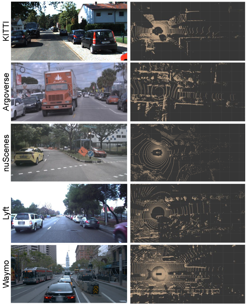
Our first goal is to understand if any biases have crept into current 3D object detectors. For this, we leverage multiple recently released datasets with similar types of sensors to KITTI [18, 19] (cameras and LiDAR) and with 3D annotations, each of them collected in different cities [3, 4, 7, 25] (see Figure 1 for an illustration). Interestingly, they are also recorded with different sensor configurations (i.e., the LiDAR and camera models as well as their mounting arrangements can be different). We first train two representative LiDAR-based 3D object detectors (PIXOR [63] and PointRCNN [52]) on each dataset and test on the others. We find that when tested on a different dataset, 3D object detectors fail dramatically: a detector trained on KITTI performs 36 percent worse on Waymo [3] compared to the one trained on Waymo. This indicates that the detector has indeed over-fitted to its training domain.

What domain differences are causing such catastrophic failure? One can think of many possibilities. There may be differences in low-level statistics of the images. The LiDAR sensors might have more or fewer beams, and may be oriented differently. But the differences can also be in the physical world being sensed. There may be differences in the number of vehicles, their orientation, and also their sizes and shapes. We present an extensive analysis of these potential biases that points to one major issue — statistical differences in the sizes and shapes of cars.

In hindsight, this difference makes sense. The best selling car in the USA is a 5-meter long truck (Ford F-series) [2], while the best selling car in Germany is a 4-meter long compact car (Volkswagen Golf¹¹1https://www.best-selling-cars.com/germany/2019-q1-germany-best-selling-car-brands-and-models/). Because of such differences, cars in KITTI tend to be smaller than cars in other datasets, a bias that 3D object detectors happily learn. As a counter to this bias, we propose an extremely simple approach that leverages aggregate statistics of car sizes (i.e., mean) to correct for this bias, in both the output annotations and the input signals. Such statistics might be acquired from the department of motor vehicles, or car sales data. This single correction results in a massive improvement in cross-dataset performance, raising the 3D easy part average precision by $41.4$ points and results in a much more robust 3D object detector.

Taken together, our contributions are two-fold:

•

We present an extensive evaluation of the domain differences between self-driving car environments and how they impact 3D detector performance. Our results suggest a single core issue: size statistics of cars in different locations.
•

We present a simple and effective approach to mitigate this issue by using easily obtainable aggregate statistics of car sizes, and show dramatic improvements in cross-dataset performance as a result.

Based on our results, we recommend that vision researchers and self-driving car companies alike be cognizant of such domain differences for large-scale deployment of 3D detection systems.

2 Related Work

We review 3D object detection for autonomous driving, and domain adaptation for 2D segmentation and detection in street scenes.

LiDAR-based detection. Most existing techniques of 3D object detection use LiDAR (sometimes with images) as the input signal, which provides accurate 3D points of the surrounding environment. The main challenge is thus on properly encoding the points so as to predict point labels or draw bounding boxes in 3D to locate objects. Frustum PointNet [41] applies PointNet [42, 43] to each frustum proposal from a 2D object detector; PointRCNN [52] learns 3D proposals from PointNet++ features [43]. MV3D [11] projects LiDAR points into frontal and bird’s-eye views (BEV) to obtain multi-view features; PIXOR [63] and LaserNet [37] show that properly encoding features in one view is sufficient to localize objects. VoxelNet [69] and PointPillar [30] encode 3D points into voxels and extracts features by 3D convolutions and PointNet. UberATG-ContFuse [34] and UberATG-MMF [33] perform continuous convolutions [56] to fuse visual and LiDAR features.

Image-based detection. While providing accurate 3D points, LiDAR sensors are notoriously expensive. A 64-line LiDAR (e.g., the one used in KITTI [19, 18]) costs around $ $75,000$ (US dollars). As an alternative, researchers have also been investigating purely image-based 3D detection. Existing algorithms are largely built upon 2D object detection [45, 20, 35], imposing extra geometric constraints [6, 8, 38, 59] to create 3D proposals. [9, 10, 39, 60] apply stereo-based depth estimation to obtain 3D coordinates of each pixel. These 3D coordinates are either entered as additional input channels into a 2D detection pipeline, or used to extract hand-crafted features. The recently proposed pseudo-LiDAR [58, 44, 66] combined stereo-based depth estimation with LiDAR-based detection, converting the depth map into a 3D point cloud and processing it exactly as LiDAR signal. The pseudo-LiDAR framework has largely improved image-based detection, yet a notable gap is still remained compared to LiDAR. In this work, we therefore focus on LiDAR-based object detectors.

Table 1: Dataset overview. We focus on their properties related to frontal-view images, LiDAR, and 3D object detection. The dataset size refers to the number of synchronized

(

image, LiDAR

)

pairs. For Waymo and nuScenes, we subsample the data. See text for details.

Dataset	Size	LiDAR Type	Beam Angles	Object Types	Rainy Weather	Night Time
KITTI [18, 19]	$14,999$	$1\times 64\text{-beam}$	$[-24^{\circ},4^{\circ}]$	8	No	No
Argoverse [7]	$22,305$	$2\times 32\text{-beam}$	$[-26^{\circ},25^{\circ}]$	17	No	Yes
nuScenes [4]	$34,149$	$1\times 32\text{-beam}$	$[-16^{\circ},11^{\circ}]$	23	Yes	Yes
Lyft [25]	$18,634$	$1\times 40\text{ or }64+2\times 40\text{-beam}$	$[-29^{\circ},5^{\circ}]$	9	No	No
Waymo [3]	$192,484$	$1\times 64+4\times 200\text{-beam}$	$[-18^{\circ},2^{\circ}]$	4	Yes	Yes

Domain adaptation. (Unsupervised) domain adaptation has also been studied in autonomous driving scenes, but mainly for the tasks of 2D semantic segmentation [13, 22, 24, 36, 48, 49, 50, 55, 67, 73] and 2D object detection [5, 12, 21, 23, 26, 27, 46, 47, 57, 72, 71]. The common setting is to adapt a model trained from one labeled source domain (e.g., synthetic images) to an unlabeled target domain (e.g., real images). The domain difference is mostly from the input signal (e.g., image styles), and many algorithms have built upon adversarial feature matching and style transfer [17, 22, 70] to minimize the domain gap in the input or feature space. Our work contrasts these methods by studying 3D object detection. We found that, the output space (e.g., car sizes) can also contribute to the domain gap; properly leveraging the statistics of the target domain can largely improve the model’s generalization ability.

3 Datasets

We review KITTI [18, 19] and introduce the other four datasets used in our experiments: Argoverse [7], Lyft [25], nuScenes [4], and Waymo [3]. We focus on data related to 3D object detection. All the datasets provide ground-truth 3D bounding box labels for several kinds of objects. We summarize the five datasets in detail in Table 1.

KITTI. The KITTI object detection benchmark [18, 19] contains $7,481$ (left) images for training and $7,518$ images for testing. The training set is further separated into $3,712$ training and $3,769$ validation images as suggested by [9]. All the scenes are pictured around Karlsruhe, Germany in clear weather and day time. For each (left) image, KITTI provides its corresponding 64-beam Velodyne LiDAR point cloud and the right stereo image.

Argoverse. The Argoverse dataset [7] is collected around Miami and Pittsburgh, USA in multiple weathers and during different times of a day. It provides images from stereo cameras and another seven cameras that cover $360^{\circ}$ information. It also provides $64$ -beam LiDAR point clouds captured by two $32$ -beam Velodyne LiDAR sensors stacked vertically. We extracted synchronized frontal-view images and corresponding point clouds from the original Argoverse dataset, with a timestamp tolerance of 51 ms between LiDAR sweeps and images. The resulting dataset we use contains $13,122$ images for training, $5,015$ images for validation, $4,168$ images for testing.

nuScenes. The nuScenes dataset [4] contains $28,130$ training and $6,019$ validation images. We treat the validation images as test images, and re-split and subsample the $28,130$ training images into $11,040$ training and $3,026$ validation images. The scenes are pictured around Boston, USA and Singapore in multiple weathers and during different times of a day. For each image, nuScenes provides the point cloud captured by a $32$ -beam roof LiDAR. It also provides images from another five cameras that cover $360^{\circ}$ information.

Lyft. The Lyft Level 5 dataset [25] contains $18,634$ frontal-view images and we separate them into $12,599$ images for training, $3,024$ images for validation, $3,011$ images for testing. The scenes are pictured around Palo Auto, USA in clear weathers and during day time. For each image, Lyft provides the point cloud captured by a $40$ (or $64$ )-beam roof LiDAR and two $40$ -beam bumper LiDAR sensors. It also provides images from another five cameras that cover $360^{\circ}$ information and one long-focal-length camera.

Waymo. The Waymo dataset [3] contains $122,000$ training, $30,407$ validation, and $40,077$ test images and we sub-sample them into $12,000$ , $3,000$ , and $3,000$ , respectively. The scenes are pictured at Phoenix, Mountain View, and San Francisco in multiple weathers and at multiple times of a day. For each image, Waymo provides the combined point cloud captured by five LiDAR sensors (one on the roof). It also provides images from another four cameras.

Data format. A non-negligible difficulty in conducting cross-dataset analysis lies in the differences of data formats. Considering that most existing algorithms are developed using the KITTI format, we transfer all the other four datasets into its format. See the Supplementary Material for details.

4 Experiments and Analysis

4.1 Setup

3D object detection algorithms. We apply two LiDAR-based models PointRCNN [52] and PIXOR [63] to detect objects in 3D by outputting the surrounding 3D bounding boxes. PIXOR represents LiDAR point clouds by 3D tensors after voxelization, while PointRCNN applies PointNet++ [43] to extract point-wise features. Both methods do not rely on images. We train both models on the five 3D object detection datasets. PointRCNN has two sub-networks, the region proposal network (RPN) and region-CNN (RCNN), that are trained separately. The RPN is trained first, for $200$ epochs with batch size $16$ and learning rate $0.02$ . The RCNN is trained for $70$ epochs with batch size $4$ and learning rate $0.02$ . We use online ground truth boxes augmentation, which copies object boxes and inside points from one scene to the same locations in another scene. For PIXOR, we train it with batch size $4$ and initial learning rate $5\times 10^{-5}$ , which will be decreased 10 times on the 50th and 80th epoch. We do randomly horizontal flip and rotate during training.

Metric. We follow KITTI to evaluate object detection in 3D and the bird’s-eye view (BEV). We focus on the Car category, which has been the main focus in existing works. We report average precision (AP) with the IoU thresholds at 0.7: a car is correctly detected if the intersection over union (IoU) with the predicted 3D box is larger than $0.7$ . We denote AP for the 3D and BEV tasks by AP ${}_{\text{3D}}$ and AP ${}_{\text{BEV}}$ .

KITTI evaluates three cases: Easy, Moderate, and Hard. Specifically, it labels each ground truth box with four levels (0 to 3) of occlusion / truncation. The Easy case contains level-0 cars whose bounding box heights in 2D are larger than $40$ pixels; the Moderate case contains level-{0, 1} cars whose bounding box heights in 2D are larger than $25$ pixels; the Hard case contains level-{0, 1, 2} cars whose bounding box heights in 2D are larger than $25$ pixels. The heights are meant to separate cars by their depths with respect to the observing car. Nevertheless, since different datasets have different image resolutions, such criteria might not be aligned across datasets. We thus replace the constraints of “larger than $40,25$ pixels” by “within $30,70$ meters”. We further evaluate cars of level-{0, 1, 2} within three depth ranges: $0-30$ , $30-50$ , and $50-70$ meters, following [63].

We mainly report and discuss results of PointRCNN on the validation set in the main paper. We report results of PIXOR in the Supplementary Material.

Table 2: 3D object detection across multiple datasets (evaluated on the validation sets). We report average precision (AP) of the Car category in bird’s-eye view (AP

{}_{\text{BEV}}

) and 3D (AP

{}_{\text{3D}}

) at

\text{IoU}=0.7

, using the PointRCNN detector [52]. We report results at different difficulties (following the KITTI benchmark, but we replace the

40

25

25

pixel thresholds on 2D bounding boxes with

30

70

70

meters on object depths, for Easy, Moderate, and Hard cases, respectively) and different depth ranges (using the same truncation and occlusion thresholds as KITTI Hard case). The results show a significant performance drop in cross-dataset inference. We indicate the best generalization results per column and per setting by red fonts and the worst by blue fonts. We indicate in-domain results by bold fonts.

Setting	Source $\backslash$ Target	KITTI	Argoverse	nuScenes	Lyft	Waymo
Easy	KITTI	88.0 / 82.5	55.8 / 27.7	47.4 / 13.3	81.7 / 51.8	45.2 / 11.9
	Argoverse	69.5 / 33.9	79.2 / 57.8	52.5 / 21.8	86.9 / 67.4	83.8 / 40.2
	nuScenes	49.7 / 13.4	73.2 / 21.8	73.4 / 38.1	89.0 / 38.2	78.8 / 36.7
	Lyft	74.3 / 39.4	77.1 / 45.8	63.5 / 23.9	90.2 / 87.3	87.0 / 64.7
	Waymo	51.9 / 13.1	76.4 / 42.6	55.5 / 21.6	87.9 / 74.5	90.1 / 85.3
Moderate	KITTI	80.6 / 68.9	44.9 / 22.3	26.2 / 8.3	61.8 / 33.7	43.9 / 12.3
	Argoverse	56.6 / 31.4	69.9 / 44.2	27.6 / 11.8	66.6 / 42.1	72.3 / 35.1
	nuScenes	39.8 / 10.7	56.6 / 17.1	40.7 / 21.2	71.4 / 25.0	68.2 / 30.8
	Lyft	61.1 / 34.3	62.5 / 35.3	33.6 / 12.3	83.7 / 65.5	77.6 / 53.2
	Waymo	45.8 / 13.2	64.4 / 29.8	28.9 / 13.7	74.2 / 53.8	85.9 / 67.9
Hard	KITTI	81.9 / 66.7	42.5 / 22.2	24.9 / 8.8	57.4 / 34.2	41.5 / 12.6
	Argoverse	58.5 / 33.3	69.9 / 42.8	26.8 / 14.5	64.4 / 42.7	68.5 / 36.8
	nuScenes	39.6 / 10.1	53.3 / 16.7	40.2 / 20.5	67.7 / 25.7	66.9 / 29.0
	Lyft	60.7 / 33.9	62.9 / 35.9	30.6 / 11.7	79.3 / 65.5	77.0 / 53.9
	Waymo	46.3 / 12.6	61.6 / 29.0	28.4 / 14.1	74.1 / 54.5	80.4 / 67.7
0-30m	KITTI	88.8 / 84.9	58.4 / 34.7	47.9 / 14.9	77.8 / 54.2	48.0 / 14.0
	Argoverse	74.2 / 46.8	83.3 / 63.3	55.3 / 26.9	87.7 / 69.5	85.7 / 44.4
	nuScenes	50.7 / 13.9	73.7 / 26.0	73.2 / 42.8	89.1 / 43.8	79.8 / 43.4
	Lyft	75.1 / 45.2	81.0 / 54.0	61.6 / 25.4	90.4 / 88.5	88.6 / 70.9
	Waymo	56.8 / 15.0	80.6 / 48.1	57.8 / 24.0	88.4 / 76.2	90.4 / 87.2
30m-50m	KITTI	70.2 / 51.4	46.5 / 19.0	9.8 / 4.5	60.1 / 34.5	50.5 / 21.4
	Argoverse	33.9 / 11.8	72.2 / 39.5	9.5 / 9.1	65.9 / 39.1	75.9 / 42.1
	nuScenes	24.1 / 3.8	46.3 / 6.4	17.1 / 4.1	70.1 / 18.9	69.4 / 29.2
	Lyft	39.3 / 16.6	59.2 / 21.8	11.2 / 9.1	83.8 / 62.7	79.4 / 55.5
	Waymo	31.7 / 9.3	58.0 / 18.8	9.9 / 9.1	74.5 / 51.4	87.5 / 68.8
50m-70m	KITTI	28.8 / 12.0	9.2 / 3.0	1.1 / 0.0	33.2 / 9.6	27.1 / 12.0
	Argoverse	10.9 / 1.3	29.9 / 6.9	0.5 / 0.0	35.1 / 14.5	46.2 / 23.0
	nuScenes	6.5 / 1.5	15.2 / 2.3	9.1 / 9.1	41.8 / 5.3	37.9 / 15.2
	Lyft	13.6 / 4.6	23.1 / 3.9	1.1 / 0.0	62.7 / 33.1	54.6 / 27.5
	Waymo	5.6 / 1.8	26.9 / 5.6	0.9 / 0.0	50.8 / 21.3	63.5 / 41.1

4.2 Results within each dataset

We first evaluate if existing 3D object detection models that have shown promising results on the KITTI benchmark can also be learned and perform well on newly released datasets. We summarize the results in Table 2: the rows are the source domains that a detector is trained on, and the columns are the target domains the detector is being tested on. The bold font indicates the within domain performance (i.e., training and testing using the same dataset).

We see that PointRCNN works fairly well on the KITTI, Lyft, and Waymo datasets, for all the easy, moderate, and hard cases. The results get slightly worse on Argoverse, and then nuScenes. We hypothesize that this may result from the relatively poor LiDAR input: nuScenes has only $32$ beams; while Argoverse has $64$ beams, every two of them are very close due to the configurations that the signal is captured by two stacked LiDAR sensors.

We further analyze at different ranges in Table 2 (bottom). We see a drastic drop on Argoverse and nuScenes for the far-away ranges, which supports our hypothesis: with fewer beams, the far-away objects can only be rendered by very sparse LiDAR points and thus are hard to detect. We also see poor accuracies at $50-70$ meters on KITTI, which may result from very few labeled training instances there.

Overall, both 3D object detection algorithms work fairly well when being trained and tested using the same dataset, as long as the input sensor signal is of high quality and the labeled instances are sufficient.

4.3 Results across datasets

We further experiment with generalizing a trained detector across datasets. We indicate the best result per column and per setting by red fonts and the worst by blue fonts.

We see a clear trend of performance drop. For instance, the PointRCNN model trained on KITTI achieves only $45.2\%$ AP ${}_{\text{BEV}}$ (Moderate) on Waymo, lower than the model trained on Waymo by over $40\%$ . The gap becomes even larger in AP ${}_{\text{3D}}$ : the same KITTI model attains only $11.9\%$ AP ${}_{\text{3D}}$ , while the Waymo model attains $85.3\%$ . We hypothesize that the car height is hard to get right. In terms of the target (test) domain, Lyft and Waymo suffer the least drop if the detector is trained from the other datasets, followed by Argoverse. KITTI and nuScenes suffer the most drop, which might result from their different geo-locations (one is from Germany and the other contains data from Singapore). The nuScenes dataset might also suffer from its relatively fewer beams in the input and other models may therefore not be able to apply. By considering different ranges, we also find that the deeper the range is, the bigger the drop is.

In terms of the source (training) domain, we see that the detector trained on KITTI seems to be the worst to transfer to others. In every $5\times 1$ block that is evaluated on a single dataset in a single setting, the KITTI model is mostly outperformed by others. Surprisingly, nuScenes model can perform fairly well when being tested on the other datasets: the results are even higher than on its own. We thus have two arguments: The quality of sensors is more important in testing than in training; KITTI data (e.g., car styles, time, and weather) might be too limited or different from others and therefore cannot transfer well to others. In the following subsections, we provide detailed analysis.

4.4 Analysis of domain idiosyncrasies

Table 2 and subsection 4.3 reveal drastic accuracy drops in generalizing 3D object detectors across datasets (domains). We hypothesize that there exist significant idiosyncrasies in each dataset. In particular, Figure 1 shows that the images and point clouds are quite different across datasets. One one hand, different datasets are collected by cars of different sensor configurations. For example, nuScenes uses a single $32$ -beam LiDAR; the point clouds are thus sparser than the other datasets. On the other hand, these datasets are collected at different locations; the environments and the foreground object styles may also be different.

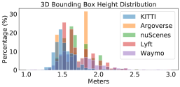
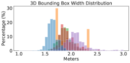
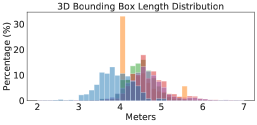
To provide a better understanding, we compute the average number of LiDAR points per scene and per car (using the ground-truth 3D bounding box) in Figure 2. We see a large difference: Waymo has ten times of points per car than nuScenes ²²2We note that PointRCNN applies point re-sampling so that every scene (in RPN) and object proposal (in RCNN) will have the same numbers of input points while PIXOR applies voxelization. Both operations can reduce but cannot fully resolve point cloud differences across domains.. We further analyze the size of bounding boxes per car. Figure 3 shows the histograms of each dataset. We again see mismatches between different datasets: KITTI seems to have the smallest box sizes while Waymo has the largest. We conduct an analysis and find that most of the bounding boxes tightly contain the points of cars inside. We, therefore, argue that this difference of box sizes is related to the car styles captured in different datasets.

4.5 Analysis of detector performance

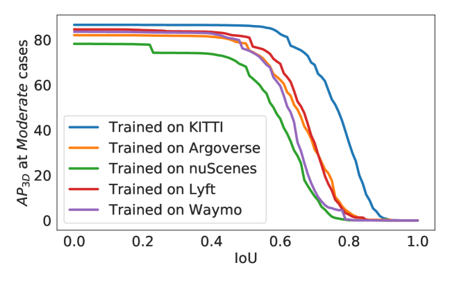
So what are the idiosyncrasies that account for the majority of performance gap? There are two factors that can lead to an miss-detected car (i.e., IoU $<0.7$ ): the car might be entirely missed by the detector, or it is detected but poorly localized. To identify the main factor, we lower down the IoU threshold using KITTI as the target domain (see Figure 5). We observe an immediate increase in AP ${}_{\text{3D}}$ , and the results become saturated when IoU is lower than $0.4$ . Surprisingly, PointRCNN models trained from other datasets perform on a par with the model trained on KITTI. In other words, poor generalization resides primarily in localization.

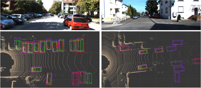
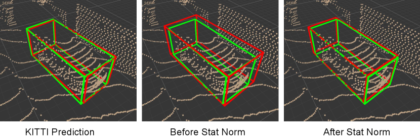
We investigate one cause of mislocalization³³3Mislocalization can result from wrong box centers, rotations, or sizes.: inaccurate box size. To this end, we replace the size of every detected car that has IoU $>0.2$ to a ground-truth car with the corresponding ground-truth box size, while keeping its bottom center and rotation unchanged. We see an immediate performance boost in Table 3 (see the Supplementary Material for complete results across all pairs of datasets). In other words, the detector trained from one domain just cannot predict the car size right in the other domains. This observation correlates with our findings in Figure 3 that these datasets have different car sizes. By further analyzing the detected boxes (in Figure 4, we apply the detector trained from Waymo to KITTI), we find that the detector tends to predict box sizes that are similar to the ground-truth sizes in source domain, even though cars in the target domain are indeed physically smaller. We think this is because the detectors trained from the source data carry the learned bias to the target data.

Table 3: Cross-dataset performance and gain (in parentheses) by assigning ground-truth box sizes to detected cars while keeping their centers and rotations unchanged. We report AP

{}_{\text{3D}}

of the Car category at

\text{IoU}=0.7

, using PointRCNN [52]. We show adaptation from KITTI to other datasets, and vice versa.

Setting	Dataset	From KITTI	To KITTI
Easy	Argoverse	65.7 (+38.0)	59.2 (+25.3)
	nuScenes	33.5 (+20.2)	63.9 (+50.5)
	Lyft	74.8 (+23.1)	58.4 (+19.0)
	Waymo	77.1 (+65.2)	78.2 (+65.1)
Moderate	Argoverse	50.9 (+28.6)	51.0 (+19.6)
	nuScenes	18.2 (+9.9)	47.3 (+36.6)
	Lyft	54.3 (+20.6)	49.4 (+15.1)
	Waymo	63.0 (+50.7)	60.6 (+47.4)
Hard	Argoverse	49.3 (+27.1)	52.5 (+19.2)
	nuScenes	17.7 (+8.9)	45.7 (+35.6)
	Lyft	53.0 (+18.8)	52.0 (+18.1)
	Waymo	59.1 (+46.5)	60.7 (+48.1)

Table 4: Improved 3D object detection across datasets (evaluated on the validation sets). We report AP

{}_{\text{BEV}}

/ AP

{}_{\text{3D}}

of the Car category at

\text{IoU}=0.7

, using PointRCNN [52]. We investigate (OT) output transformation by directly adjusting the predicted box sizes, (SN) statistical normalization, and (FS) few-shot fine-tuning (with

10

labeled instances). We also include (Direct) directly applying the detectors trained on the source domain and (Within) applying the detectors trained on the target domain for comparison. We show adaption results from KITTI to other datasets, and vice versa. We mark the best result among Direct, OT, SN, and FS in red fonts, and worst in blue fonts.

		From KITTI (KITTI as the source; others as the target)					To KITTI (KITTI as the target; others as the source)
Setting	Dataset	Direct	OT	SN	FS	Within	Direct	OT	SN	FS	Within
Easy	Argoverse	55.8 / 27.7	72.7 / 9.0	74.7 / 48.2	75.8 / 49.2	79.2 / 57.8	69.5 / 33.9	53.3 / 5.7	76.2 / 46.1	80.0 / 49.7	88.0 / 82.5
	nuScenes	47.4 / 13.3	55.0 / 10.4	60.8 / 23.9	54.7 / 21.7	73.4 / 38.1	49.7 / 13.4	75.4 / 31.5	83.2 / 35.6	83.8 / 58.7	88.0 / 82.5
	Lyft	81.7 / 51.8	88.2 / 23.5	88.3 / 73.3	89.0 / 78.1	90.2 / 87.3	74.3 / 39.4	71.9 / 4.7	83.5 / 72.1	85.3 / 72.5	88.0 / 82.5
	Waymo	45.2 / 11.9	86.1 / 16.2	84.6 / 53.3	87.4 / 70.9	90.1 / 85.3	51.9 / 13.1	64.0 / 3.9	82.1 / 48.7	81.0 / 67.0	88.0 / 82.5
Mod.	Argoverse	44.9 / 22.3	59.9 / 7.9	61.5 / 38.2	60.7 / 37.3	69.9 / 44.2	56.6 / 31.4	52.2 / 7.3	67.2 / 40.5	68.8 / 42.8	80.6 / 68.9
	nuScenes	26.2 / 8.3	30.8 / 6.8	32.9 / 16.4	28.7 / 12.5	40.7 / 21.2	39.8 / 10.7	58.5 / 27.3	67.4 / 31.0	67.2 / 45.5	80.6 / 68.9
	Lyft	61.8 / 33.7	70.1 / 17.8	73.7 / 53.1	74.2 / 53.4	83.7 / 65.5	61.1 / 34.3	60.8 / 5.6	73.6 / 57.9	73.9 / 56.2	80.6 / 68.9
	Waymo	43.9 / 12.3	69.1 / 13.1	74.9 / 49.4	75.9 / 55.3	85.9 / 67.9	45.8 / 13.2	54.9 / 3.7	71.3 / 47.1	66.8 / 51.8	80.6 / 68.9
Hard	Argoverse	42.5 / 22.2	59.3 / 9.3	60.6 / 37.1	59.8 / 36.5	69.9 / 42.8	58.5 / 33.3	53.5 / 8.6	68.5 / 41.9	66.3 / 43.0	81.9 / 66.7
	nuScenes	24.9 / 8.8	27.8 / 7.6	31.9 / 15.8	27.5 / 12.4	40.2 / 20.5	39.6 / 10.1	59.5 / 27.8	65.2 / 30.8	64.7 / 44.5	81.9 / 66.7
	Lyft	57.4 / 34.2	66.5 / 19.1	73.1 / 53.5	71.8 / 52.9	79.3 / 65.5	60.7 / 33.9	63.1 / 6.9	75.2 / 58.9	74.1 / 56.2	81.9 / 66.7
	Waymo	41.5 / 12.6	68.7 / 13.9	69.4 / 49.4	70.1 / 54.4	80.4 / 67.7	46.3 / 12.6	58.0 / 4.1	73.0 / 49.7	68.1 / 52.9	81.9 / 66.7
0-30	Argoverse	58.4 / 34.7	73.0 / 13.7	73.1 / 54.2	73.6 / 55.2	83.3 / 63.3	74.2 / 46.8	64.9 / 10.1	83.3 / 53.9	84.0 / 56.9	88.8 / 84.9
	nuScenes	47.9 / 14.9	56.2 / 13.9	60.0 / 29.2	54.0 / 23.6	73.2 / 42.8	50.7 / 13.9	74.6 / 36.6	83.6 / 42.8	81.2 / 59.8	88.8 / 84.9
	Lyft	77.8 / 54.2	88.4 / 27.5	88.8 / 75.4	89.3 / 77.6	90.4 / 88.5	75.1 / 45.2	74.8 / 9.1	87.4 / 73.6	87.5 / 73.9	88.8 / 84.9
	Waymo	48.0 / 14.0	87.7 / 22.2	87.1 / 60.1	88.7 / 74.1	90.4 / 87.2	56.8 / 15.0	71.3 / 4.4	85.7 / 59.0	84.8 / 71.0	88.8 / 84.9
30-50	Argoverse	46.5 / 19.0	56.1 / 5.4	61.5 / 31.5	59.0 / 29.9	72.2 / 39.5	33.9 / 11.8	35.1 / 9.1	48.9 / 25.7	47.9 / 23.8	70.2 / 51.4
	nuScenes	9.8 / 4.5	10.8 / 9.1	11.0 / 2.3	9.5 / 6.1	17.1 / 4.1	24.1 / 3.8	35.5 / 15.5	44.9 / 18.6	45.0 / 25.1	70.2 / 51.4
	Lyft	60.1 / 34.5	67.4 / 10.7	73.8 / 52.2	73.7 / 50.4	83.8 / 62.7	39.3 / 16.6	43.3 / 3.9	58.3 / 38.0	57.7 / 33.3	70.2 / 51.4
	Waymo	50.5 / 21.4	73.6 / 10.4	78.1 / 54.9	78.1 / 57.2	87.5 / 68.8	31.7 / 9.3	39.8 / 4.5	57.3 / 36.3	49.2 / 29.2	70.2 / 51.4
50-70	Argoverse	9.2 / 3.0	20.5 / 1.0	23.8 / 5.6	20.1 / 6.3	29.9 / 6.9	10.9 / 1.3	8.0 / 0.8	9.1 / 2.6	8.1 / 3.8	28.8 / 12.0
	nuScenes	1.1 / 0.0	1.5 / 1.0	3.0 / 2.3	3.3 / 1.2	9.1 / 9.1	6.5 / 1.5	7.8 / 5.1	9.4 / 5.1	12.9 / 5.7	28.8 / 12.0
	Lyft	33.2 / 9.6	41.3 / 6.8	49.9 / 22.2	46.8 / 19.4	62.7 / 33.1	13.6 / 4.6	12.7 / 0.9	21.1 / 6.7	17.5 / 8.0	28.8 / 12.0
	Waymo	27.1 / 12.0	42.6 / 4.2	46.8 / 25.1	45.2 / 24.3	63.5 / 41.1	5.6 / 1.8	7.7 / 1.1	14.4 / 5.7	10.5 / 4.8	28.8 / 12.0

5 Domain Adaptation Approaches

The poor performance due to mislocalization rather than misdetection opens the possibility of adapting a learned detector to a new domain with relatively smaller efforts. We investigate two scenarios: (1) a few labeled scenes (i.e., point clouds with 3D box annotations) or (2) the car size statistics of the target domain are available. We argue that both scenarios are practical: we can simply annotate for every place a few labeled instances, or get the statistics from the local vehicle offices or car-selling websites. In the main paper, we will mainly focus on training from KITTI and testing on the others, and vice versa. We leave other results in the Supplementary Material.

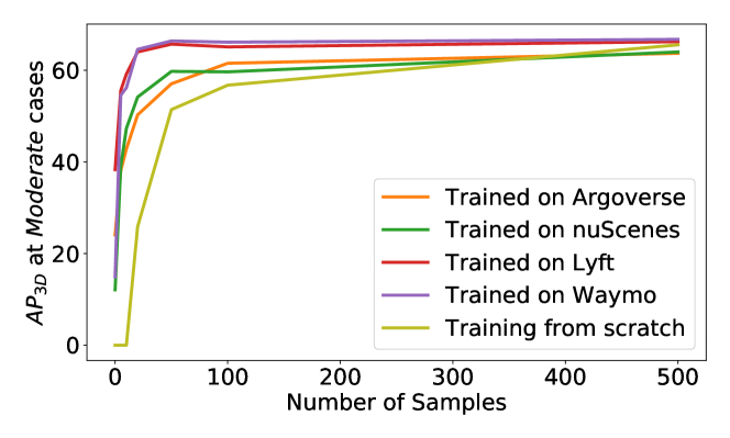
Few-shot (FS) fine-tuning. In the first scenario where a few labeled scenes from the target domain are accessible, we investigate fine-tuning the already trained object detector with these few-shot examples. As shown in Table 4, using only $10$ labeled scenes (average over five rounds of experiments) of the target domain, we can already improve the AP ${}_{\text{3D}}$ by over $20.4\%$ on average when adapting KITTI to other datasets and $24.4\%$ on average when adapting other datasets to KITTI. Figure 6 further shows the performance by fine-tuning with different number of scenes. With merely $20$ labeled target scenes, the adapted detector from Lyft and Waymo can already be on a par with that trained from scratch in the target domain with $500$ scenes.

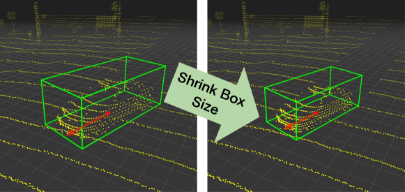
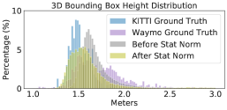
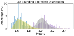
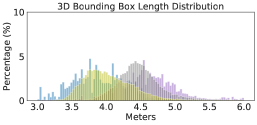
Statistical normalization (SN). For the second scenario where the target statistics (i.e., average height, width, and length of cars) are accessible, we investigate modifying the already trained object detector so that its predicted box sizes can better match the target statistics. We propose a data modification scheme named statistical normalization by adjusting the source domain data, as illustrated in Figure 7. Specifically, we compute the difference of mean car sizes between the target domain (TD) and source domain (SD), $\Delta=(\Delta h,\Delta w,\Delta l)=(h_{\text{TD}},w_{\text{TD}},L_{\text{TD}})-(h_{\text{SD}},w_{\text{SD}},L_{\text{SD}})$ , where $h,w,l$ stand for the height, width, and length, respectively⁴⁴4Here we obtain the target statistics directly from the dataset. We investigate using the car sales data online in the Supplementary Material.. We then modify both the point clouds and the labels in the source domain with respect to $\Delta$ . For each annotated bounding box of cars, we adjust its size by adding $(\Delta h,\Delta w,\Delta l)$ . We also crop the points inside the original box, scale up or shrink their coordinates to fit the adjusted bounding box size accordingly, and paste them back to the point cloud of the scene. By doing so, we generate new point clouds and labels whose car sizes are much similar to the target domain data. We then fine-tune the already trained model on the source domain with these data.

Surprisingly, with such a simple method that does not requires labeled target domain data, the performance is significantly improved (see Table 4) between KITTI and other datasets that obviously contain cars of different styles (i.e., one in Germany, and others in the USA). Figure 4 and Figure 8 further analyze the prediction before and after statistical normalization. We see a clear shift of the histogram (predicted box) from the source to the target domain.

Output transformation (OT). We investigate an even simpler approach by directly adjusting the detector’s prediction without fine-tuning — by adding $(\Delta h,\Delta w,\Delta l)$ to the predicted size. As shown in Table 4, this approach does not always improve but sometimes degrade the accuracy. This is because when we apply the source detector to the target domain, the predicted box sizes do slightly deviate from the source statistics to the target ones due to the difference of object sizes in the input signals (see Figure 4). Thus, simply adding $(\Delta h,\Delta w,\Delta l)$ may over-correct the bias. We hypothesize that by searching a suitable scale for addition or designing more intelligent output transformations can alleviate this problem and we leave them for future work.

Discussion. As shown in Table 4, statistical normalization largely improves over direct applying the source-domain detector. For some pairs of data sets (e.g., from KITTI to Lyft, the AP ${}_{\text{BEV}}$ after statistical normalization is encouraging, largely closing the gap to the Within performance.

Compared to domain adaptation on 2D images, there are more possible factors of domain gaps in 3D. While the box size difference is just one factor, we find addressing it to be highly effective in closing the gaps. This factor is rarely discussed in other domain adaptation tasks. We thus expect it and our solution to be valuable additions to the community.

6 Conclusion

In conclusion, in this paper we are the first (to our knowledge) to provide and investigate a standardized form of most widely-used 3D object detection datasets for autonomous driving. Although naïve adaptation across datasets is unsurprisingly difficult, we observe that, surprisingly, there appears to be a single dominant factor that explains a majority share of the adaptation gap: varying car sizes across different geographic regions. That car sizes play such an important role in adaptation ultimately makes sense. No matter if the detection is based on LiDAR or stereo cameras, cars are only observed from one side — and the depth of the bounding boxes must be estimated based on experience. If a deep network trained in Germany encounters an American Ford F-Series truck (with $5.3$ m length), it has little chance to correctly estimate the corresponding bounding box. It is surprising, however, that just matching the mean size of cars in the areas during fine-tuning already reduces this uncertainty so much. We hope that this publication will kindle interests in the exciting problem of cross-dataset domain adaptation for 3D object detection and localization, and that researchers will be careful to first apply simple global corrections before developing new computer vision algorithms to tackle the remaining adaptation gap.

Acknowledgments

This research is supported by grants from the National Science Foundation NSF (III-1618134, III-1526012, IIS-1149882, IIS-1724282, OAC-1934714, and TRIPODS-1740822), the Office of Naval Research DOD (N00014-17-1-2175), the Bill and Melinda Gates Foundation, and the Cornell Center for Materials Research with funding from the NSF MRSEC program (DMR-1719875). We are thankful for generous support by Zillow and SAP America Inc.

References

[1] https://en.wikipedia.org/wiki/Death_of_Elaine_Herzberg, 2018.
[2] https://www.motor1.com/features/280320/20-bestselling-vehicles-2018/, 2018.
[3] Waymo open dataset: An autonomous driving dataset, 2019.
[4] Holger Caesar, Varun Bankiti, Alex H. Lang, Sourabh Vora, Venice Erin Liong, Qiang Xu, Anush Krishnan, Yu Pan, Giancarlo Baldan, and Oscar Beijbom. nuscenes: A multimodal dataset for autonomous driving. arXiv preprint arXiv:1903.11027, 2019.
[5] Qi Cai, Yingwei Pan, Chong-Wah Ngo, Xinmei Tian, Lingyu Duan, and Ting Yao. Exploring object relation in mean teacher for cross-domain detection. In CVPR, 2019.
[6] Florian Chabot, Mohamed Chaouch, Jaonary Rabarisoa, Céline Teulière, and Thierry Chateau. Deep manta: A coarse-to-fine many-task network for joint 2d and 3d vehicle analysis from monocular image. In CVPR, 2017.
[7] Ming-Fang Chang, John W Lambert, Patsorn Sangkloy, Jagjeet Singh, Slawomir Bak, Andrew Hartnett, De Wang, Peter Carr, Simon Lucey, Deva Ramanan, and James Hays. Argoverse: 3d tracking and forecasting with rich maps. In CVPR, 2019.
[8] Xiaozhi Chen, Kaustav Kundu, Ziyu Zhang, Huimin Ma, Sanja Fidler, and Raquel Urtasun. Monocular 3d object detection for autonomous driving. In CVPR, 2016.
[9] Xiaozhi Chen, Kaustav Kundu, Yukun Zhu, Andrew G Berneshawi, Huimin Ma, Sanja Fidler, and Raquel Urtasun. 3d object proposals for accurate object class detection. In NIPS, 2015.
[10] Xiaozhi Chen, Kaustav Kundu, Yukun Zhu, Huimin Ma, Sanja Fidler, and Raquel Urtasun. 3d object proposals using stereo imagery for accurate object class detection. TPAMI, 40(5):1259–1272, 2018.
[11] Xiaozhi Chen, Huimin Ma, Ji Wan, Bo Li, and Tian Xia. Multi-view 3d object detection network for autonomous driving. In CVPR, 2017.
[12] Yuhua Chen, Wen Li, Christos Sakaridis, Dengxin Dai, and Luc Van Gool. Domain adaptive faster r-cnn for object detection in the wild. In CVPR, 2018.
[13] Yuhua Chen, Wen Li, and Luc Van Gool. Road: Reality oriented adaptation for semantic segmentation of urban scenes. In CVPR, 2018.
[14] Yilun Chen, Shu Liu, Xiaoyong Shen, and Jiaya Jia. Fast point r-cnn. In ICCV, 2019.
[15] Yilun Chen, Shu Liu, Xiaoyong Shen, and Jiaya Jia. Dsgn: Deep stereo geometry network for 3d object detection. In CVPR, 2020.
[16] Xinxin Du, Marcelo H Ang Jr, Sertac Karaman, and Daniela Rus. A general pipeline for 3d detection of vehicles. In ICRA, 2018.
[17] Yaroslav Ganin, Evgeniya Ustinova, Hana Ajakan, Pascal Germain, Hugo Larochelle, François Laviolette, Mario Marchand, and Victor Lempitsky. Domain-adversarial training of neural networks. JMLR, 17(1):2096–2030, 2016.
[18] Andreas Geiger, Philip Lenz, Christoph Stiller, and Raquel Urtasun. Vision meets robotics: The kitti dataset. The International Journal of Robotics Research, 32(11):1231–1237, 2013.
[19] Andreas Geiger, Philip Lenz, and Raquel Urtasun. Are we ready for autonomous driving? the kitti vision benchmark suite. In CVPR, 2012.
[20] Kaiming He, Georgia Gkioxari, Piotr Dollár, and Ross Girshick. Mask r-cnn. In ICCV, 2017.
[21] Zhenwei He and Lei Zhang. Multi-adversarial faster-rcnn for unrestricted object detection. In ICCV, 2019.
[22] Judy Hoffman, Eric Tzeng, Taesung Park, Jun-Yan Zhu, Phillip Isola, Kate Saenko, Alexei A Efros, and Trevor Darrell. Cycada: Cycle-consistent adversarial domain adaptation. In ICML, 2018.
[23] Han-Kai Hsu, Chun-Han Yao, Yi-Hsuan Tsai, Wei-Chih Hung, Hung-Yu Tseng, Maneesh Singh, and Ming-Hsuan Yang. Progressive domain adaptation for object detection. In WACV, 2020.
[24] Haoshuo Huang, Qixing Huang, and Philipp Krahenbuhl. Domain transfer through deep activation matching. In ECCV, 2018.
[25] R. Kesten, M. Usman, J. Houston, T. Pandya, K. Nadhamuni, A. Ferreira, M. Yuan, B. Low, A. Jain, P. Ondruska, S. Omari, S. Shah, A. Kulkarni, A. Kazakova, C. Tao, L. Platinsky, W. Jiang, and V. Shet. Lyft level 5 av dataset 2019. urlhttps://level5.lyft.com/dataset/, 2019.
[26] Mehran Khodabandeh, Arash Vahdat, Mani Ranjbar, and William G Macready. A robust learning approach to domain adaptive object detection. In ICCV, 2019.
[27] Taekyung Kim, Minki Jeong, Seunghyeon Kim, Seokeon Choi, and Changick Kim. Diversify and match: A domain adaptive representation learning paradigm for object detection. In CVPR, 2019.
[28] Hendrik Königshof, Niels Ole Salscheider, and Christoph Stiller. Realtime 3d object detection for automated driving using stereo vision and semantic information. In 2019 IEEE Intelligent Transportation Systems Conference (ITSC), 2019.
[29] Jason Ku, Melissa Mozifian, Jungwook Lee, Ali Harakeh, and Steven Waslander. Joint 3d proposal generation and object detection from view aggregation. In IROS, 2018.
[30] Alex H Lang, Sourabh Vora, Holger Caesar, Lubing Zhou, Jiong Yang, and Oscar Beijbom. Pointpillars: Fast encoders for object detection from point clouds. In CVPR, 2019.
[31] Buyu Li, Wanli Ouyang, Lu Sheng, Xingyu Zeng, and Xiaogang Wang. Gs3d: An efficient 3d object detection framework for autonomous driving. In CVPR, 2019.
[32] Peiliang Li, Xiaozhi Chen, and Shaojie Shen. Stereo r-cnn based 3d object detection for autonomous driving. In CVPR, 2019.
[33] Ming Liang, Bin Yang, Yun Chen, Rui Hu, and Raquel Urtasun. Multi-task multi-sensor fusion for 3d object detection. In CVPR, 2019.
[34] Ming Liang, Bin Yang, Shenlong Wang, and Raquel Urtasun. Deep continuous fusion for multi-sensor 3d object detection. In ECCV, 2018.
[35] Tsung-Yi Lin, Piotr Dollár, Ross B Girshick, Kaiming He, Bharath Hariharan, and Serge J Belongie. Feature pyramid networks for object detection. In CVPR, 2017.
[36] Yawei Luo, Liang Zheng, Tao Guan, Junqing Yu, and Yi Yang. Taking a closer look at domain shift: Category-level adversaries for semantics consistent domain adaptation. In CVPR, 2019.
[37] Gregory P Meyer, Ankit Laddha, Eric Kee, Carlos Vallespi-Gonzalez, and Carl K Wellington. Lasernet: An efficient probabilistic 3d object detector for autonomous driving. In CVPR, 2019.
[38] Arsalan Mousavian, Dragomir Anguelov, John Flynn, and Jana Košecká. 3d bounding box estimation using deep learning and geometry. In CVPR, 2017.
[39] Cuong Cao Pham and Jae Wook Jeon. Robust object proposals re-ranking for object detection in autonomous driving using convolutional neural networks. Signal Processing: Image Communication, 53:110–122, 2017.
[40] Alex D Pon, Jason Ku, Chengyao Li, and Steven L Waslander. Object-centric stereo matching for 3d object detection. In ICRA, 2020.
[41] Charles R Qi, Wei Liu, Chenxia Wu, Hao Su, and Leonidas J Guibas. Frustum pointnets for 3d object detection from rgb-d data. In CVPR, 2018.
[42] Charles R Qi, Hao Su, Kaichun Mo, and Leonidas J Guibas. Pointnet: Deep learning on point sets for 3d classification and segmentation. In CVPR, 2017.
[43] Charles Ruizhongtai Qi, Li Yi, Hao Su, and Leonidas J Guibas. Pointnet++: Deep hierarchical feature learning on point sets in a metric space. In NIPS, 2017.
[44] Rui Qian, Divyansh Garg, Yan Wang, Yurong You, Serge Belongie, Bharath Hariharan, Mark Campbell, Kilian Q Weinberger, and Wei-Lun Chao. End–end pseudo-lidar for image-based 3d object detection. In CVPR, 2020.
[45] Shaoqing Ren, Kaiming He, Ross Girshick, and Jian Sun. Faster r-cnn: Towards real-time object detection with region proposal networks. In NIPS, 2015.
[46] Adrian Lopez Rodriguez and Krystian Mikolajczyk. Domain adaptation for object detection via style consistency. In BMVC, 2019.
[47] Kuniaki Saito, Yoshitaka Ushiku, Tatsuya Harada, and Kate Saenko. Strong-weak distribution alignment for adaptive object detection. In CVPR, 2019.
[48] Kuniaki Saito, Kohei Watanabe, Yoshitaka Ushiku, and Tatsuya Harada. Maximum classifier discrepancy for unsupervised domain adaptation. In CVPR, 2018.
[49] Fatemeh Sadat Saleh, Mohammad Sadegh Aliakbarian, Mathieu Salzmann, Lars Petersson, and Jose M Alvarez. Effective use of synthetic data for urban scene semantic segmentation. In ECCV. Springer, 2018.
[50] Swami Sankaranarayanan, Yogesh Balaji, Arpit Jain, Ser Nam Lim, and Rama Chellappa. Learning from synthetic data: Addressing domain shift for semantic segmentation. In CVPR, 2018.
[51] Shaoshuai Shi, Chaoxu Guo, Li Jiang, Zhe Wang, Jianping Shi, Xiaogang Wang, and Hongsheng Li. Pv-rcnn: Point-voxel feature set abstraction for 3d object detection. In CVPR, 2020.
[52] Shaoshuai Shi, Xiaogang Wang, and Hongsheng Li. Pointrcnn: 3d object proposal generation and detection from point cloud. In CVPR, 2019.
[53] Shaoshuai Shi, Zhe Wang, Jianping Shi, Xiaogang Wang, and Hongsheng Li. From points to parts: 3d object detection from point cloud with part-aware and part-aggregation network. TPAMI, 2020.
[54] Weijing Shi and Ragunathan Rajkumar. Point-gnn: Graph neural network for 3d object detection in a point cloud. In CVPR, 2020.
[55] Yi-Hsuan Tsai, Wei-Chih Hung, Samuel Schulter, Kihyuk Sohn, Ming-Hsuan Yang, and Manmohan Chandraker. Learning to adapt structured output space for semantic segmentation. In CVPR, 2018.
[56] Shenlong Wang, Simon Suo, Wei-Chiu Ma3 Andrei Pokrovsky, and Raquel Urtasun. Deep parametric continuous convolutional neural networks. In CVPR, 2018.
[57] Tao Wang, Xiaopeng Zhang, Li Yuan, and Jiashi Feng. Few-shot adaptive faster r-cnn. In CVPR, 2019.
[58] Yan Wang, Wei-Lun Chao, Divyansh Garg, Bharath Hariharan, Mark Campbell, and Kilian Q. Weinberger. Pseudo-lidar from visual depth estimation: Bridging the gap in 3d object detection for autonomous driving. In CVPR, 2019.
[59] Yu Xiang, Wongun Choi, Yuanqing Lin, and Silvio Savarese. Subcategory-aware convolutional neural networks for object proposals and detection. In WACV, 2017.
[60] Bin Xu and Zhenzhong Chen. Multi-level fusion based 3d object detection from monocular images. In CVPR, 2018.
[61] Zhenbo Xu, Wei Zhang, Xiaoqing Ye, Xiao Tan, Wei Yang, Shilei Wen, Errui Ding, Ajin Meng, and Liusheng Huang. Zoomnet: Part-aware adaptive zooming neural network for 3d object detection. 2020.
[62] Yan Yan, Yuxing Mao, and Bo Li. Second: Sparsely embedded convolutional detection. Sensors, 18(10):3337, 2018.
[63] Bin Yang, Wenjie Luo, and Raquel Urtasun. Pixor: Real-time 3d object detection from point clouds. In CVPR, 2018.
[64] Zetong Yang, Yanan Sun, Shu Liu, and Jiaya Jia. 3dssd: Point-based 3d single stage object detector. In CVPR, 2020.
[65] Zetong Yang, Yanan Sun, Shu Liu, Xiaoyong Shen, and Jiaya Jia. Std: Sparse-to-dense 3d object detector for point cloud. In ICCV, 2019.
[66] Yurong You, Yan Wang, Wei-Lun Chao, Divyansh Garg, Geoff Pleiss, Bharath Hariharan, Mark Campbell, and Kilian Q Weinberger. Pseudo-lidar++: Accurate depth for 3d object detection in autonomous driving. In ICLR, 2020.
[67] Yang Zhang, Philip David, and Boqing Gong. Curriculum domain adaptation for semantic segmentation of urban scenes. In ICCV, 2017.
[68] Yin Zhou, Pei Sun, Yu Zhang, Dragomir Anguelov, Jiyang Gao, Tom Ouyang, James Guo, Jiquan Ngiam, and Vijay Vasudevan. End-to-end multi-view fusion for 3d object detection in lidar point clouds. In CoRL, 2019.
[69] Yin Zhou and Oncel Tuzel. Voxelnet: End-to-end learning for point cloud based 3d object detection. In CVPR, 2018.
[70] Jun-Yan Zhu, Taesung Park, Phillip Isola, and Alexei A Efros. Unpaired image-to-image translation using cycle-consistent adversarial networks. In ICCV, 2017.
[71] Xinge Zhu, Jiangmiao Pang, Ceyuan Yang, Jianping Shi, and Dahua Lin. Adapting object detectors via selective cross-domain alignment. In CVPR, 2019.
[72] Chenfan Zhuang, Xintong Han, Weilin Huang, and Matthew R Scott. ifan: Image-instance full alignment networks for adaptive object detection. In AAAI, 2020.
[73] Yang Zou, Zhiding Yu, BVK Vijaya Kumar, and Jinsong Wang. Unsupervised domain adaptation for semantic segmentation via class-balanced self-training. In ECCV, 2018.

Supplementary Material

In this Supplementary Material, we provide details omitted in the main paper.

•

Appendix S1: data format conversion (section 3 of the main paper).
•

Appendix S2: evaluation metric (subsection 4.1 of the main paper).
•

Appendix S3: additional results on dataset discrepancy (subsection 4.4 and subsection 4.5 of the main paper).
•

Appendix S4: object detection using PIXOR [63] (subsection 4.2 and subsection 4.3 of the main paper).
•

Appendix S5: object detection using PointRCNN with different adaptation methods (subsection 4.5 and section 5 of the main paper).
•

Appendix S6: additional qualitative results (section 5 of the main paper).

Appendix S1 Converting Datasets into KITTI Format

In this section we describe in detail how we convert Argoverse [7], nuScenes [4], Lyft [25], and Waymo [3] into KITTI [18, 19] format. As the formatting of images, point clouds and camera calibration information is trivial, and label fields such as $alpha$ and $rotation_{y}$ have been well-defined, we only discuss the labeling process with non-deterministic definitions.

S1.1 Object filtering

Due to the fact that KITTI focuses on objects that appear in the camera view, we follow its setting and discard all object annotations outside the frontal camera view. To allow truncated objects, we project the 8 corners of each object’s 3D bounding box onto the image plane. An object will be discarded if all its 8 corners fall out of the image boundary. To make other datasets consistent with KITTI, we do not consider labeled objects farther than $70$ meters.

S1.2 Matching categories with KITTI

Since the taxonomy of object categories among datasets are misaligned, it is necessary to re-label each dataset in the same way as KITTI does. As we focus on car detection, here we describe how we construct the new car and truck categories for each dataset except KITTI in Table S5. The truck category is also important since detected trucks are treated as false positives when we look at the car category. We would like to point out that Waymo labels all kinds of vehicles as cars. A model trained on Waymo thus will tend to predict trucks or other vehicles as cars. Therefore, directly applying a model trained on Waymo to other datasets will lead to higher false positive rates. For other datasets, the definition between categories can vary (e.g., Argoverse label Ford F-Series as cars; nuScenes labels some as trucks) and result in cross-domain accuracy drop even if the data are collected at similar locations with similar sensors.

Table S5: The original categories in each dataset that we include into the car and truck categories following the KITTI label formulation.

Dataset	Car	Truck
Argoverse	{VEHICLE}	{LARGE_VEHICLE, BUS, TRAILER, SCHOOL_BUS}
nuScenes	{car}	{bus, trailer, construction_vehicle, truck}
Lyft	{Car}	{other_vehicle, truck, bus, emergency_vehicle}
Waymo	{Car}	$\varnothing$

S1.3 Handling missing 2D bounding boxes

To annotate each object in the image with a 2D bounding box (the information is used by the original KITTI metric), we first compute 8 corners of its 3D bounding box, and then calculate their pixel coordinates $\{(cx_{n},cy_{n}),1\leq n\leq 8\}$ . We then draw the smallest bounding box $(x_{1},y_{1},x_{2},y_{2})$ that contains all corners whose projections fall in the image plane:

$\displaystyle x_{1}$	$\displaystyle=\max(\mathop{\min}_{0\leq n<8}cx_{n},0),$
$\displaystyle y_{1}$	$\displaystyle=\max(\mathop{\min}_{0\leq n<8}cy_{n},0),$
$\displaystyle x_{2}$	$\displaystyle=\min(\mathop{\max}_{0\leq n<8}cx_{n},width),$	(1)
$\displaystyle y_{2}$	$\displaystyle=\min(\mathop{\max}_{0\leq n<8}cy_{n},height),$

where $width$ and $height$ denote the width and height of the 2D image, respectively.

S1.4 Calculating truncation values

Following the KITTI formulation, the truncation value refers to how much of an object locates beyond image boundary. With Equation 1 we estimate it by calculating how much of the object’s 2D uncropped bounding box is outside the image boundary:

$\displaystyle x_{1}^{\prime}$	$\displaystyle=\mathop{\min}_{0\leq n<8}cx_{n},$
$\displaystyle y_{1}^{\prime}$	$\displaystyle=\mathop{\min}_{0\leq n<8}cy_{n},$
$\displaystyle x_{2}^{\prime}$	$\displaystyle=\mathop{\max}_{0\leq n<8}cx_{n},$	(2)
$\displaystyle y_{2}^{\prime}$	$\displaystyle=\mathop{\max}_{0\leq n<8}cy_{n},$
truncation	$\displaystyle=1-\frac{(x_{2}-x_{1})\times(y_{2}-y_{1})}{(x_{2}^{\prime}-x_{1}^{\prime})\times(y_{2}^{\prime}-y_{1}^{\prime})}.$

S1.5 Calculating occlusion values

We estimate the occlusion value of objects by approximating car shapes with corresponding 2D bounding boxes. The occlusion value is thus derived by computing the percentage of pixels occluded by bounding boxes from closer objects. We discretize the $0\text{--}1$ occlusion value into KITTI’s $\{0,1,2,3\}$ labels by equally dividing the interval into 4 parts. We describe in algorithm 1 the detail of how we compute occlusion value for each object.

Input : Image height

H

, image width

W

, object list

objs

canvas\leftarrow Array([H,W])

;

2 for $x\in\{0,1,\dots,W-1\}$ do

3 for $y\in\{0,1,\dots,H-1\}$ do

canvas[x,y]\leftarrow-1

;

objs\leftarrow Sort(objs,key=depth,order=descending)

;

8 for $obj\in objs$ do

[x_{1},x_{2},y_{1},y_{2}]=obj.bounding\_bbox

;

10 for $x\in\{x_{1},x_{1}+1,\dots,x_{2}-1\}$ do

11 for $y\in\{y_{1},y_{1}+1,\dots,y_{2}-1\}$ do

canvas[x,y]\leftarrow obj.id

;

16for $obj\in objs$ do

[x_{1},x_{2},y_{1},y_{2}]=obj.bounding\_bbox

;

cnt\leftarrow 0

;

19 for $x\in\{x_{1},x_{1}+1,\dots,x_{2}-1\}$ do

20 for $y\in\{y_{1},y_{1}+1,\dots,y_{2}-1\}$ do

21 if $canvas[x,y]=obj.id$ then

cnt\leftarrow cnt+1

;

obj.occlusion\leftarrow 1-\frac{cnt}{(x_{2}-x_{1})\times(y_{2}-y_{1})}

;

Algorithm 1 Computing occlusion of objects from a single scene

Table S6: 3D object detection results across multiple datasets using the original KITTI evaluation metric (pixel thresholds). We apply PointRCNN [52]. We report average precision (AP) of the Car category in bird’s-eye view and 3D (AP

{}_{\text{BEV}}

/ AP

{}_{\text{3D}}

\text{IoU}=0.7

) and compare object detection accuracy of different difficulties. The results are less comparable due to misaligned difficulty partitions among datasets. Red color: best generalization (per column and per setting); blue color: worst generalization; bold font: within-domain results.

Setting	Source $\backslash$ Target	KITTI	Argoverse	nuScenes	Lyft	Waymo
Easy	KITTI	88.0 / 82.3	44.2 / 21.4	27.5 / 7.1	72.3 / 45.5	42.1 / 10.6
	Argoverse	68.6 / 31.5	69.9 / 43.6	28.3 / 11.4	76.8 / 56.4	73.5 / 34.2
	nuScenes	49.4 / 13.2	57.0 / 16.5	43.4 / 21.3	83.0 / 31.8	71.7 / 28.2
	Lyft	72.6 / 38.9	66.9 / 33.2	35.5 / 13.1	86.4 / 77.1	78.0 / 54.6
	Waymo	52.0 / 13.1	64.9 / 29.4	31.5 / 14.3	82.5 / 68.8	85.3 / 71.7
Moderate	KITTI	86.0 / 74.7	44.9 / 22.3	26.2 / 8.3	63.2 / 36.3	43.9 / 12.3
	Argoverse	65.2 / 36.6	69.8 / 44.2	27.6 / 11.8	68.5 / 43.6	72.1 / 35.1
	nuScenes	45.4 / 12.1	56.5 / 17.1	40.7 / 21.2	73.4 / 26.3	68.1 / 30.7
	Lyft	67.3 / 38.3	62.4 / 35.3	33.6 / 12.3	79.6 / 66.8	77.3 / 53.1
	Waymo	51.5 / 14.9	64.4 / 29.8	28.9 / 13.7	75.5 / 58.2	85.6 / 67.9
Hard	KITTI	85.7 / 74.8	42.5 / 22.2	24.9 / 8.8	62.0 / 34.9	41.4 / 12.6
	Argoverse	63.5 / 37.8	69.8 / 42.8	26.8 / 14.5	65.9 / 44.4	68.5 / 36.7
	nuScenes	42.2 / 11.1	53.2 / 16.7	40.2 / 20.5	73.0 / 27.8	66.8 / 29.0
	Lyft	65.0 / 37.0	62.8 / 35.8	30.6 / 11.7	79.7 / 67.3	76.6 / 53.8
	Waymo	48.9 / 14.4	61.6 / 29.0	28.4 / 14.1	75.5 / 55.8	80.2 / 67.6

Table S7: Percentage (%) of data (total annotated cars with depths

\in[0,70]

meters) in each difficult partition with old / new difficulty metric. The new easy threshold selects much fewer data than the old metric on all datasets except KITTI.

	Dataset	Easy	Moderate	Hard
Training Set	KITTI	21.7 / 21.6	55.5 / 67.8	76.1 / 91.0
	Argoverse	27.7 / 14.9	40.5 / 40.5	59.6 / 59.6
	nuScenes	31.9 / 13.9	47.2 / 47.2	64.8 / 64.8
	Lyft	25.0 / 15.5	50.4 / 54.9	64.9 / 70.5
	Waymo	29.0 / 10.7	40.1 / 40.1	58.7 / 58.7
Validation Set	KITTI	20.4 / 20.4	55.4 / 65.5	77.1 / 88.4
	Argoverse	29.2 / 14.3	41.7 / 41.7	60.6 / 60.6
	nuScenes	38.3 / 18.4	53.6 / 53.6	68.5 / 68.5
	Lyft	25.3 / 15.5	52.5 / 57.7	66.9 / 73.3
	Waymo	30.3 / 10.3	42.3 / 42.3	60.9 / 60.9

Appendix S2 The New Difficulty Metric

In subsection 4.1 of the main paper, we develop a new difficulty metric to evaluate object detection (i.e., how to define easy, moderate, and hard cases) so as to better align different datasets. Concretely, KITTI defines its easy, moderate, and hard cases according to truncation, occlusion, and 2D bounding box height (in pixels) of ground-truth annotations. The 2D box height (the threshold at 40 pixels) is meant to differentiate far-away and nearby objects: the easy cases only contain nearby objects. However, since the datasets we compare are collected using cameras of different focal lengths and contain images of different resolutions, directly applying the KITTI definition may not well align datasets. For example, a car at $50$ meters is treated as a moderate case in KITTI but may be treated as a easy case in other datasets.

To resolve this issue, we re-define detection difficulty based on object truncation, occlusion, and depth range (in meters), which completely removes the influences of cameras. In developing this new metric we hope to achieve similar case partitions to the original metric of KITTI. To this end, we estimate the distance thresholds with

D=\frac{f_{v}\times H}{h},

(3)

where $D$ denotes depth, $f_{v}$ denotes vertical camera focal length, and $H$ and $h$ are object height in the 3D camera space and the 2D image space, respectively. For a car of average height ( $1.53$ meters) in KITTI, the corresponding depth for $40$ pixels is $27.03$ meters. We therefore select $30$ meters as the new threshold to differentiate easy from moderate and hard cases. For moderate and hard cases, we disregard cars with depths larger than $70$ meters since most of the annotated cars in KITTI are within this range. Table S7 shows the comparison between old and new difficulty partitions. The new metric contains fewer easy cases than the old metric for all but the KITTI dataset. This is because that the other datasets use either larger focal lengths or resolutions: the objects in images are therefore larger than in KITTI. We note that, the moderate cases contain all the easy cases, and the hard cases contain all the easy and moderate cases.

We also report in Table S6 the detection results within and across datasets using the old metric, in comparison to Table 2 of the main paper which uses the new metric. One notable difference is that for the easy cases in the old metric, both the within and across domain performances drop for all but KITTI datasets, since many far-away cars (which are hard to detect) in the other datasets are treated as easy cases in the old metric.

Appendix S3 Dataset discrepancy

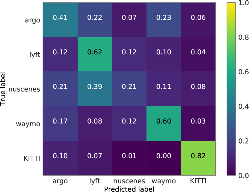
We have shown the box size distributions of each dataset in Figure 3 of the main paper. We also calculate the mean of the bounding box sizes in Table S8. There is a huge gap of size between KITTI and the other four datasets. In addition, we train an SVM classifier with the RBF kernel to predict which dataset a bounding box belongs to and present the confusion matrix result in Figure S9 (row: ground truth; column: prediction). The model has a very high confidence to distinguish KITTI from the other datasets.

Table S8: The average size (meters) of 3D ground truth bounding boxes of the five datasets.

Dataset	Width	Height	Length
KITTI	1.62	1.53	3.89
Argoverse	1.96	1.69	4.51
nuScenes	1.96	1.73	4.64
Lyft	1.91	1.71	4.73
Waymo	2.11	1.79	4.80

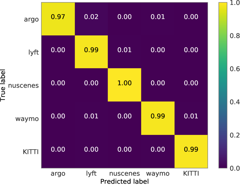
We further train a point cloud classifier to tell which dataset a point cloud of car belongs to, using PointNet++ [43] as the backbone. For each dataset, we sample 8,000 object point cloud instances as training examples and 1,000 as testing examples. We show the confusion matrix in Figure S10. The classifier can almost perfectly classify the point clouds. Compared to Figure S9, we argue that not only the bounding box sizes, but also the point cloud styles (e.g., density, number of laser beams, etc) of cars contribute to dataset discrepancy. Interestingly, while the second factor seems to be more informative in differentiating datasets, the first factor is indeed the main cause of poor transfer performance among datasets⁵⁵5As mentioned in the main paper, PointRCNN applies point re-sampling so that every scene (in RPN) and object proposal (in RCNN) will have the same numbers of input points. Such an operation could reduce the point cloud differences across domains..

Appendix S4 PIXOR Results

We report object detection results using PXIOR [63], which takes voxelized tensors instead of point clouds as input. We implement the algorithm ourselves, achieving comparable results as the ones in [63]. We report the results in Table S9. PXIOR performs pretty well if the model is trained and tested within the same dataset, suggesting that its model design does not over-fit to KITTI.

We also see a clear performance drop when we train a model on one dataset and test it on the other datasets. The drop is more severe than applying the PointRCNN detector in many cases. We surmise that the re-sampling operation used in PointRCNN might make the difference. We therefore apply the same re-sampling operation on the input point cloud before inputting it to PIXOR. Table S10 shows the results: re-sampling does improve the performance in applying the Waymo detector to other datasets. This is likely because Waymo has the most LiDAR points on average and re-sampling reduces the number, making it more similar to that of the other datasets. We expect that tuning the number of points in re-sampling can further boost the performance.

Table S9: 3D object detection across multiple datasets (evaluated on the validation sets). We report average precision (AP) of the Car category in the bird’s-eye view (AP

{}_{\text{BEV}}

) at

\text{IoU}=0.7

, using PIXOR [63]. We report results at different difficulties (following the KITTI benchmark, but we replace the

40

25

25

pixel thresholds on 2D bounding boxes with

30

70

70

Setting	Source $\backslash$ Target	KITTI	Argoverse	nuScenes	Lyft	Waymo
Easy	KITTI	87.2	31.5	39.4	65.1	28.3
	Argoverse	57.4	79.2	49.0	89.4	69.3
	nuScenes	40.4	66.3	56.8	79.7	40.7
	Lyft	53.1	71.4	45.5	90.7	75.2
	Waymo	9.8	63.6	38.1	82.5	87.2
Moderate	KITTI	72.8	25.9	20.0	37.4	23.4
	Argoverse	42.5	67.3	24.4	57.9	55.0
	nuScenes	30.3	46.3	30.1	50.5	35.3
	Lyft	38.7	58.5	24.9	78.1	56.8
	Waymo	10.0	47.4	21.0	62.4	76.4
Hard	KITTI	68.2	28.4	18.8	34.5	24.1
	Argoverse	43.0	64.7	22.7	57.7	55.2
	nuScenes	27.1	46.0	29.8	50.6	35.8
	Lyft	35.8	54.3	24.8	78.0	53.7
	Waymo	11.1	46.9	21.3	63.4	74.8
0-30m	KITTI	87.2	39.5	38.9	62.2	32.1
	Argoverse	60.0	82.4	49.9	88.0	72.8
	nuScenes	38.7	63.0	55.1	79.4	43.9
	Lyft	50.7	73.5	48.4	90.5	76.4
	Waymo	12.9	65.7	42.7	83.1	88.3
30m-50m	KITTI	50.3	29.4	9.1	31.0	26.1
	Argoverse	23.7	66.1	0.8	54.5	56.5
	nuScenes	18.6	44.9	12.3	48.1	37.3
	Lyft	17.5	50.4	7.0	77.0	53.0
	Waymo	8.1	41.3	4.5	62.1	78.0
50m-70m	KITTI	12.0	3.0	3.0	9.0	10.1
	Argoverse	4.8	31.7	0.3	20.6	31.3
	nuScenes	9.1	13.4	9.1	21.6	20.9
	Lyft	6.5	19.1	9.1	61.2	29.9
	Waymo	1.7	20.6	9.1	39.7	53.3

Table S10: 3D object detection across multiple datasets (evaluated on the validation sets). The setting is exactly the same as Table S9, except that we perform PointRCNN re-sampling on the input point cloud before applying the PIXOR detector.

Setting	Source $\backslash$ Target	KITTI	Argoverse	nuScenes	Lyft	Waymo
Easy	KITTI	85.9	22.3	35.7	56.2	13.4
	Argoverse	59.4	80.5	47.1	89.3	66.5
	nuScenes	14.5	57.1	66.2	73.4	44.2
	Lyft	66.6	73.8	52.2	90.7	77.3
	Waymo	28.6	66.0	52.0	84.2	86.7
Moderate	KITTI	70.3	19.1	18.9	33.5	14.8
	Argoverse	43.0	66.5	24.1	57.9	52.6
	nuScenes	12.6	46.9	36.5	52.6	35.7
	Lyft	49.3	54.4	28.6	79.4	59.2
	Waymo	23.8	51.4	26.7	69.0	77.1
Hard	KITTI	67.2	20.0	17.4	33.1	15.0
	Argoverse	42.8	63.8	22.3	57.7	52.5
	nuScenes	14.4	44.6	35.7	53.1	36.0
	Lyft	45.5	54.5	27.6	79.3	58.5
	Waymo	24.0	54.2	26.4	70.3	77.3
0-30m	KITTI	85.8	28.6	33.2	56.6	14.7
	Argoverse	61.5	82.7	48.6	88.3	65.0
	nuScenes	20.2	61.5	64.4	75.4	48.4
	Lyft	62.9	71.9	54.3	90.7	78.3
	Waymo	31.0	65.9	55.4	85.9	88.2
30m-50m	KITTI	48.8	22.0	4.5	29.3	16.8
	Argoverse	21.1	69.7	2.3	55.1	54.6
	nuScenes	8.6	42.8	15.9	52.7	40.5
	Lyft	25.1	53.1	10.3	78.6	59.9
	Waymo	16.7	52.4	9.8	68.8	78.8
50m-70m	KITTI	15.7	3.4	0.4	7.5	12.0
	Argoverse	9.4	29.5	0.1	22.2	30.4
	nuScenes	0.7	12.8	9.1	23.1	16.4
	Lyft	7.3	18.8	3.0	63.6	30.8
	Waymo	2.3	23.5	9.1	45.1	56.8

Appendix S5 Additional Results Using PointRCNN

S5.1 Complete tables

We show the complete tables across five datasets by replacing the predicted box sizes with the ground truth sizes (cf. subsection 4.5 in the main paper) in Table S11, by few-shot fine-tuning in Table S12, by statistical normalization in Table S13, and by output transformation in Table S14. For statistical normalization and output transformation, we see smaller improvements (or even some degradation) among datasets collected in the USA than between datasets collected in Germany and the USA.

Table S11: Cross-dataset performance by assigning ground-truth box sizes to detected cars while keeping their centers and rotations unchanged. We report AP

{}_{\text{BEV}}

/ AP

{}_{\text{3D}}

of the Car category at

\text{IoU}=0.7

, using PointRCNN [52]. We indicate the best generalization results per column and per setting by red fonts and the worst by blue fonts. We indicate in-domain results by bold fonts.

Setting	Source $\backslash$ Target	KITTI	Argoverse	nuScenes	Lyft	Waymo
Easy	KITTI	95.6 / 84.6	80.5 / 65.7	66.5 / 33.5	89.8 / 74.8	90.3 / 77.1
	Argoverse	80.0 / 59.2	83.1 / 77.3	54.2 / 26.7	87.5 / 75.6	89.1 / 74.7
	nuScenes	80.5 / 63.9	77.4 / 52.5	74.8 / 46.4	89.4 / 65.2	85.6 / 62.9
	Lyft	83.9 / 58.4	80.2 / 67.2	65.2 / 29.2	90.3 / 87.3	89.9 / 73.9
	Waymo	86.1 / 78.2	79.2 / 72.7	63.1 / 30.0	88.3 / 86.1	90.2 / 86.2
Moderate	KITTI	81.4 / 72.6	64.5 / 50.9	35.0 / 18.2	74.6 / 54.3	79.4 / 63.0
	Argoverse	66.9 / 51.0	73.6 / 60.1	28.2 / 17.6	67.6 / 52.3	77.3 / 61.5
	nuScenes	61.4 / 47.3	59.0 / 36.2	41.7 / 25.4	72.4 / 45.1	69.2 / 50.6
	Lyft	71.4 / 49.4	68.5 / 49.3	34.6 / 17.4	84.2 / 66.9	79.7 / 64.7
	Waymo	73.7 / 60.6	68.0 / 54.9	30.8 / 18.4	75.0 / 63.2	86.4 / 74.4
Hard	KITTI	82.5 / 71.9	64.0 / 49.3	31.4 / 17.7	73.1 / 53.0	77.2 / 59.1
	Argoverse	65.6 / 52.5	73.6 / 59.2	27.5 / 16.6	65.3 / 52.2	75.8 / 58.4
	nuScenes	61.3 / 45.7	55.3 / 33.5	40.9 / 25.4	72.6 / 43.6	68.3 / 46.2
	Lyft	72.0 / 52.0	65.4 / 49.8	31.2 / 16.5	84.8 / 67.2	78.2 / 63.6
	Waymo	75.3 / 60.7	67.8 / 51.9	30.2 / 17.0	75.2 / 61.9	80.8 / 68.9
0-30m	KITTI	89.2 / 86.7	82.3 / 70.2	62.8 / 35.1	89.8 / 76.2	90.4 / 78.7
	Argoverse	83.3 / 68.7	86.1 / 80.2	56.8 / 31.9	88.3 / 77.3	89.8 / 78.1
	nuScenes	76.5 / 62.5	80.9 / 55.2	74.2 / 49.1	89.4 / 67.7	87.5 / 62.6
	Lyft	86.7 / 62.7	84.2 / 69.3	63.1 / 31.7	90.5 / 88.5	90.2 / 77.2
	Waymo	88.0 / 75.8	82.8 / 76.3	62.0 / 32.9	88.7 / 86.8	90.5 / 88.1
30m-50m	KITTI	71.6 / 56.4	63.1 / 40.4	11.1 / 9.1	74.3 / 52.9	80.4 / 64.3
	Argoverse	43.2 / 27.0	74.5 / 53.9	9.5 / 9.1	67.4 / 49.3	78.8 / 62.9
	nuScenes	37.1 / 25.0	49.0 / 18.3	17.4 / 10.4	71.0 / 42.2	75.4 / 50.5
	Lyft	52.8 / 31.4	61.9 / 35.6	11.3 / 9.1	85.1 / 65.9	80.4 / 65.4
	Waymo	57.6 / 38.5	63.5 / 45.8	10.0 / 9.1	75.4 / 62.5	87.7 / 74.9
50m-70m	KITTI	30.8 / 15.1	23.6 / 9.7	1.6 / 1.0	50.0 / 24.0	53.3 / 31.2
	Argoverse	13.7 / 10.1	34.2 / 11.7	0.5 / 0.0	37.2 / 19.8	51.9 / 31.7
	nuScenes	9.2 / 5.7	15.8 / 4.3	9.8 / 9.1	46.9 / 20.1	43.4 / 23.2
	Lyft	17.2 / 8.1	28.2 / 11.4	1.1 / 0.1	64.2 / 39.9	57.8 / 36.3
	Waymo	13.1 / 4.9	29.2 / 11.4	0.9 / 0.0	53.0 / 29.4	65.9 / 45.2

Table S12: Cross-dataset performance by few-shot fine-tuning using

10

labeled target domain instances (average over five rounds of experiments). We report AP

{}_{\text{BEV}}

/ AP

{}_{\text{3D}}

of the Car category at

\text{IoU}=0.7

, using PointRCNN [52]. We indicate the best generalization results per column and per setting by red fonts and the worst by blue fonts. We indicate in-domain results by bold fonts.

Setting	Source $\backslash$ Target	KITTI	Argoverse	nuScenes	Lyft	Waymo
Easy	KITTI	88.0 / 82.5	75.8 / 49.2	54.7 / 21.7	89.0 / 78.1	87.4 / 70.9
	Argoverse	80.0 / 49.7	74.2 / 42.0	54.0 / 19.2	86.6 / 63.5	86.6 / 56.3
	nuScenes	83.8 / 58.7	68.7 / 33.7	73.4 / 38.1	88.4 / 67.7	84.3 / 59.8
	Lyft	85.3 / 72.5	73.5 / 48.9	56.5 / 17.7	90.2 / 87.3	89.1 / 70.4
	Waymo	81.0 / 67.0	76.9 / 55.2	51.0 / 16.7	88.3 / 81.0	90.1 / 85.3
Moderate	KITTI	80.6 / 68.9	60.7 / 37.3	28.7 / 12.5	74.2 / 53.4	75.9 / 55.3
	Argoverse	68.8 / 42.8	66.5 / 34.4	27.5 / 11.2	65.4 / 40.2	75.3 / 46.7
	nuScenes	67.2 / 45.5	54.5 / 24.2	40.7 / 21.2	71.9 / 44.0	72.8 / 47.0
	Lyft	73.9 / 56.2	61.0 / 35.3	30.3 / 10.6	83.7 / 65.5	78.3 / 57.9
	Waymo	66.8 / 51.8	65.7 / 41.8	26.7 / 11.0	75.1 / 54.8	85.9 / 67.9
Hard	KITTI	81.9 / 66.7	59.8 / 36.5	27.5 / 12.4	71.8 / 52.9	70.1 / 54.4
	Argoverse	66.3 / 43.0	67.9 / 37.3	26.9 / 11.8	66.0 / 42.0	70.3 / 43.9
	nuScenes	64.7 / 44.5	52.0 / 23.4	40.2 / 20.5	71.0 / 44.3	68.7 / 44.3
	Lyft	74.1 / 56.2	61.9 / 37.0	28.6 / 11.1	79.3 / 65.5	76.9 / 55.6
	Waymo	68.1 / 52.9	62.3 / 39.3	26.7 / 11.7	74.7 / 55.2	80.4 / 67.7
0-30m	KITTI	88.8 / 84.9	73.6 / 55.2	54.0 / 23.6	89.3 / 77.6	88.7 / 74.1
	Argoverse	84.0 / 56.9	81.2 / 52.2	54.0 / 22.6	87.7 / 68.7	88.3 / 60.7
	nuScenes	81.2 / 59.8	70.5 / 40.1	73.2 / 42.8	88.8 / 69.6	86.2 / 62.4
	Lyft	87.5 / 73.9	78.1 / 54.3	56.9 / 21.2	90.4 / 88.5	89.4 / 74.8
	Waymo	84.8 / 71.0	79.4 / 56.6	52.8 / 20.8	88.8 / 79.1	90.4 / 87.2
30m-50m	KITTI	70.2 / 51.4	59.0 / 29.9	9.5 / 6.1	73.7 / 50.4	78.1 / 57.2
	Argoverse	47.9 / 23.8	70.8 / 34.0	7.3 / 2.0	65.4 / 36.9	78.1 / 48.5
	nuScenes	45.0 / 25.1	51.4 / 17.1	17.1 / 4.1	71.5 / 41.5	74.2 / 48.0
	Lyft	57.7 / 33.3	62.4 / 29.5	6.5 / 3.3	83.8 / 62.7	79.7 / 59.9
	Waymo	49.2 / 29.2	60.6 / 34.7	9.4 / 6.3	75.1 / 52.6	87.5 / 68.8
50m-70m	KITTI	28.8 / 12.0	20.1 / 6.3	3.3 / 1.2	46.8 / 19.4	45.2 / 24.3
	Argoverse	8.1 / 3.8	33.0 / 12.7	0.4 / 0.0	38.0 / 10.3	51.1 / 23.4
	nuScenes	12.9 / 5.7	15.5 / 2.6	9.1 / 9.1	47.0 / 14.9	44.3 / 19.3
	Lyft	17.5 / 8.0	26.8 / 9.1	2.5 / 0.0	62.7 / 33.1	54.0 / 27.2
	Waymo	10.5 / 4.8	27.6 / 7.3	1.3 / 0.0	51.2 / 19.9	63.5 / 41.1

Table S13: Cross-dataset performance by fine-tuning with source data after statistical normalization. We report AP

{}_{\text{BEV}}

/ AP

{}_{\text{3D}}

of the Car category at

\text{IoU}=0.7

, using PointRCNN [52]. We indicate the best generalization results per column and per setting by red fonts and the worst by blue fonts. We indicate in-domain results by bold fonts.

Setting	Source $\backslash$ Target	KITTI	Argoverse	nuScenes	Lyft	Waymo
Easy	KITTI	88.0 / 82.5	74.7 / 48.2	60.8 / 23.9	88.3 / 73.3	84.6 / 53.3
	Argoverse	76.2 / 46.1	79.2 / 57.8	48.3 / 18.6	84.8 / 65.0	84.8 / 49.2
	nuScenes	83.2 / 35.6	72.0 / 25.3	73.4 / 38.1	88.7 / 38.1	76.6 / 43.3
	Lyft	83.5 / 72.1	74.4 / 44.0	57.8 / 21.1	90.2 / 87.3	86.3 / 66.4
	Waymo	82.1 / 48.7	75.0 / 44.4	54.9 / 20.7	85.7 / 80.0	90.1 / 85.3
Moderate	KITTI	80.6 / 68.9	61.5 / 38.2	32.9 / 16.4	73.7 / 53.1	74.9 / 49.4
	Argoverse	67.2 / 40.5	69.9 / 44.2	24.7 / 11.1	63.3 / 38.9	72.0 / 43.6
	nuScenes	67.4 / 31.0	55.6 / 17.9	40.7 / 21.2	71.1 / 24.5	66.6 / 32.2
	Lyft	73.6 / 57.9	59.7 / 33.3	30.4 / 10.9	83.7 / 65.5	75.5 / 51.3
	Waymo	71.3 / 47.1	62.3 / 31.7	28.8 / 11.5	71.5 / 52.6	85.9 / 67.9
Hard	KITTI	81.9 / 66.7	60.6 / 37.1	31.9 / 15.8	73.1 / 53.5	69.4 / 49.4
	Argoverse	68.5 / 41.9	69.9 / 42.8	24.3 / 10.9	61.6 / 40.2	68.2 / 42.7
	nuScenes	65.2 / 30.8	52.5 / 17.2	40.2 / 20.5	67.3 / 28.6	65.7 / 30.4
	Lyft	75.2 / 58.9	60.8 / 31.8	29.5 / 14.4	79.3 / 65.5	75.5 / 53.2
	Waymo	73.0 / 49.7	60.2 / 32.5	28.4 / 10.9	71.6 / 53.3	80.4 / 67.7
0-30m	KITTI	88.8 / 84.9	73.1 / 54.2	60.0 / 29.2	88.8 / 75.4	87.1 / 60.1
	Argoverse	83.3 / 53.9	83.3 / 63.3	51.5 / 23.0	86.3 / 68.4	87.3 / 59.7
	nuScenes	83.6 / 42.8	72.8 / 27.2	73.2 / 42.8	88.9 / 47.1	78.5 / 45.9
	Lyft	87.4 / 73.6	78.7 / 51.8	58.7 / 26.8	90.4 / 88.5	87.9 / 72.4
	Waymo	85.7 / 59.0	79.9 / 50.5	57.6 / 24.3	87.2 / 75.8	90.4 / 87.2
30m-50m	KITTI	70.2 / 51.4	61.5 / 31.5	11.0 / 2.3	73.8 / 52.2	78.1 / 54.9
	Argoverse	48.9 / 25.7	72.2 / 39.5	5.0 / 4.5	61.0 / 32.4	74.4 / 46.2
	nuScenes	44.9 / 18.6	45.6 / 7.3	17.1 / 4.1	70.1 / 18.1	67.9 / 31.6
	Lyft	58.3 / 38.0	57.2 / 18.5	6.5 / 4.5	83.8 / 62.7	77.2 / 52.4
	Waymo	57.3 / 36.3	54.9 / 20.1	9.1 / 1.5	71.3 / 48.4	87.5 / 68.8
50m-70m	KITTI	28.8 / 12.0	23.8 / 5.6	3.0 / 2.3	49.9 / 22.2	46.8 / 25.1
	Argoverse	9.1 / 2.6	29.9 / 6.9	0.2 / 0.1	28.9 / 8.8	46.2 / 21.2
	nuScenes	9.4 / 5.1	14.8 / 2.3	9.1 / 9.1	40.7 / 5.2	36.4 / 14.9
	Lyft	21.1 / 6.7	21.2 / 4.9	4.5 / 0.0	62.7 / 33.1	52.1 / 25.3
	Waymo	14.4 / 5.7	27.7 / 11.0	1.0 / 0.0	46.9 / 22.0	63.5 / 41.1

Table S14: Cross-dataset performance by output transformation: directly adjusting the predicted box size by adding the difference of mean sizes between domains. We report AP

{}_{\text{BEV}}

/ AP

{}_{\text{3D}}

of the Car category at

\text{IoU}=0.7

, using PointRCNN [52]. We indicate the best generalization results per column and per setting by red fonts and the worst by blue fonts. We indicate in-domain results by bold fonts.

Setting	Source $\backslash$ Target	KITTI	Argoverse	nuScenes	Lyft	Waymo
Easy	KITTI	88.0 / 82.5	72.7 / 9.0	55.0 / 10.4	88.2 / 23.5	86.1 / 16.2
	Argoverse	53.3 / 5.7	79.2 / 57.8	52.6 / 21.3	87.1 / 66.1	87.6 / 56.1
	nuScenes	75.4 / 31.5	73.3 / 27.9	73.4 / 38.1	89.2 / 44.3	78.4 / 35.5
	Lyft	71.9 / 4.7	77.1 / 48.0	63.1 / 24.5	90.2 / 87.3	89.2 / 73.9
	Waymo	64.0 / 3.9	74.3 / 54.8	58.8 / 25.2	88.3 / 85.3	90.1 / 85.3
Moderate	KITTI	80.6 / 68.9	59.9 / 7.9	30.8 / 6.8	70.1 / 17.8	69.1 / 13.1
	Argoverse	52.2 / 7.3	69.9 / 44.2	27.5 / 11.7	66.9 / 42.1	74.3 / 45.5
	nuScenes	58.5 / 27.3	56.8 / 20.4	40.7 / 21.2	71.3 / 27.3	67.8 / 26.2
	Lyft	60.8 / 5.6	62.7 / 37.6	33.5 / 12.5	83.7 / 65.5	78.4 / 60.8
	Waymo	54.9 / 3.7	62.9 / 40.4	30.1 / 14.5	74.3 / 59.8	85.9 / 67.9
Hard	KITTI	81.9 / 66.7	59.3 / 9.3	27.8 / 7.6	66.5 / 19.1	68.7 / 13.9
	Argoverse	53.5 / 8.6	69.9 / 42.8	26.7 / 14.5	64.6 / 43.0	70.0 / 44.2
	nuScenes	59.5 / 27.8	53.6 / 19.9	40.2 / 20.5	67.6 / 28.5	66.3 / 26.0
	Lyft	63.1 / 6.9	63.4 / 38.6	30.4 / 13.3	79.3 / 65.5	77.3 / 57.3
	Waymo	58.0 / 4.1	60.5 / 39.2	29.4 / 14.6	74.0 / 57.2	80.4 / 67.7
0-30m	KITTI	88.8 / 84.9	73.0 / 13.7	56.2 / 13.9	88.4 / 27.5	87.7 / 22.2
	Argoverse	64.9 / 10.1	83.3 / 63.3	55.2 / 27.0	87.8 / 69.9	87.9 / 62.6
	nuScenes	74.6 / 36.6	73.7 / 32.0	73.2 / 42.8	89.2 / 46.2	79.6 / 41.6
	Lyft	74.8 / 9.1	81.2 / 55.8	61.2 / 27.2	90.4 / 88.5	89.6 / 77.2
	Waymo	71.3 / 4.4	78.4 / 55.7	60.5 / 25.8	88.7 / 85.0	90.4 / 87.2
30m-50m	KITTI	70.2 / 51.4	56.1 / 5.4	10.8 / 9.1	67.4 / 10.7	73.6 / 10.4
	Argoverse	35.1 / 9.1	72.2 / 39.5	9.5 / 0.3	66.3 / 39.1	77.5 / 44.9
	nuScenes	35.5 / 15.5	47.4 / 7.8	17.1 / 4.1	69.9 / 22.5	68.7 / 21.1
	Lyft	43.3 / 3.9	60.8 / 25.4	11.2 / 9.1	83.8 / 62.7	79.5 / 61.4
	Waymo	39.8 / 4.5	58.1 / 34.9	9.9 / 9.1	74.5 / 57.5	87.5 / 68.8
50m-70m	KITTI	28.8 / 12.0	20.5 / 1.0	1.5 / 1.0	41.3 / 6.8	42.6 / 4.2
	Argoverse	8.0 / 0.8	29.9 / 6.9	0.5 / 0.0	35.6 / 14.2	49.2 / 20.3
	nuScenes	7.8 / 5.1	15.3 / 3.0	9.1 / 9.1	41.4 / 5.6	37.0 / 12.0
	Lyft	12.7 / 0.9	25.6 / 6.0	1.1 / 0.0	62.7 / 33.1	54.9 / 30.4
	Waymo	7.7 / 1.1	25.5 / 6.5	0.9 / 0.0	50.8 / 22.3	63.5 / 41.1

S5.2 Online sales data

In the main paper, for statistical normalization we leverage the average car size of each dataset. Here we collect car sales data from Germany and the USA in the past four years. The average car size $(h,w,l)$ is $(1.75,1.93,5.15)$ in the USA and $(1.49,1.79,4.40)$ in Germany. The difference is $(0.26,0.14,0.75)$ , not far from $(0.20,0.37,0.78)$ between KITTI and the other datasets. The gap can be reduced by further considering locations (e.g., Argoverse from Miami and Pittsburgh, USA) and earlier data (KITTI was collected in 2011).

In Table S15, we show the results of adapting a detector trained on KITTI to other datasets using statistical normalization with the car sales data: $(\Delta h,\Delta w,\Delta l)$ is $(0.26,0.15,0.75)$ . The performance is slightly worse than using the statistics of the datasets. Nevertheless, compared to directly applying the source domain detector, statistical normalization with the car sales data still shows notable improvements.

Table S15: Statistical normalization using the mean sizes of datasets versus car sales data. Direct: directly applying the source domain detector.

		From KITTI (KITTI as the source)
Setting	Dataset	Direct	Datasets	Car sales data
Easy	Argoverse	55.8 / 27.7	74.7 / 48.2	68.6 / 32.8
	nuScenes	47.4 / 13.3	60.8 / 23.9	62.0 / 24.4
	Lyft	81.7 / 51.8	88.3 / 73.3	88.9 / 69.9
	Waymo	45.2 / 11.9	84.6 / 53.3	66.7 / 22.8
Moderate	Argoverse	44.9 / 22.3	61.5 / 38.2	57.7 / 29.1
	nuScenes	26.2 / 8.3	32.9 / 16.4	32.6 / 13.0
	Lyft	61.8 / 33.7	73.7 / 53.1	72.6 / 47.6
	Waymo	43.9 / 12.3	74.9 / 49.4	61.8 / 22.9
Hard	Argoverse	42.5 / 22.2	60.6 / 37.1	54.0 / 30.0
	nuScenes	24.9 / 8.8	31.9 / 15.8	29.8 / 13.2
	Lyft	57.4 / 34.2	73.1 / 53.5	71.7 / 45.7
	Waymo	41.5 / 12.6	69.4 / 49.4	62.7 / 25.1
0-30m	Argoverse	58.4 / 34.7	73.1 / 54.2	71.0 / 44.0
	nuScenes	47.9 / 14.9	60.0 / 29.2	60.1 / 26.1
	Lyft	77.8 / 54.2	88.8 / 75.4	89.2 / 72.5
	Waymo	48.0 / 14.0	87.1 / 60.1	72.4 / 30.2
30m-50m	Argoverse	46.5 / 19.0	61.5 / 31.5	57.4 / 20.0
	nuScenes	9.8 / 4.5	11.0 / 2.3	5.7 / 3.0
	Lyft	60.1 / 34.5	73.8 / 52.2	72.2 / 42.7
	Waymo	50.5 / 21.4	78.1 / 54.9	66.8 / 35.5
50m-70m	Argoverse	9.2 / 3.0	23.8 / 5.6	16.8 / 4.5
	nuScenes	1.1 / 0.0	3.0 / 2.3	1.0 / 0.1
	Lyft	33.2 / 9.6	49.9 / 22.2	46.0 / 18.8
	Waymo	27.1 / 12.0	46.8 / 25.1	44.2 / 18.0

S5.3 Pedestrian

We calculate the statistics of pedestrians, as in Table S16. There are smaller differences among datasets. We therefore expect a smaller improvement by statistical normalization.

Table S16: Dataset statistics on pedestrians (meters)

	KITTI	Argoverse	nuScenes	Lyft	Waymo
H	1.76 $\pm$ 0.11	1.84 $\pm$ 0.15	1.78 $\pm$ 0.18	1.76 $\pm$ 0.18	1.75 $\pm$ 0.20
W	0.66 $\pm$ 0.14	0.78 $\pm$ 0.14	0.67 $\pm$ 0.14	0.76 $\pm$ 0.14	0.85 $\pm$ 0.15
L	0.84 $\pm$ 0.23	0.78 $\pm$ 0.14	0.73 $\pm$ 0.19	0.78 $\pm$ 0.17	0.90 $\pm$ 0.19

Appendix S6 Qualitative Results

We further show qualitative results of statistical normalization refinement. We train a PointRCNN detector on Waymo and test it on KITTI. We compare its car detection before and after statistical normalization refinement in Figure S11. Statistical normalization can not only improve the predicted bounding box sizes, but also reduce false positive rates.