Tracing Privacy Leakage of Language Models to Training Data via Adjusted Influence Functions
Abstract
The responses generated by Large Language Models (LLMs) can include sensitive information from individuals and organizations, leading to potential privacy leakage. This work implements Influence Functions (IFs) to trace privacy leakage back to the training data, thereby mitigating privacy concerns of Language Models (LMs). However, we notice that current IFs struggle to accurately estimate the influence of tokens with large gradient norms, potentially overestimating their influence. When tracing the most influential samples, this leads to frequently tracing back to samples with large gradient norm tokens, overshadowing the actual most influential samples even if their influences are well estimated. To address this issue, we propose Heuristically Adjusted IF (HAIF), which reduces the weight of tokens with large gradient norms, thereby significantly improving the accuracy of tracing the most influential samples. To establish easily obtained groundtruth for tracing privacy leakage, we construct two datasets, PII-E and PII-CR, representing two distinct scenarios: one with identical text in the model outputs and pre-training data, and the other where models leverage their reasoning abilities to generate text divergent from pre-training data. HAIF significantly improves tracing accuracy, enhancing it by 20.96% to 73.71% on the PII-E dataset and 3.21% to 45.93% on the PII-CR dataset, compared to the best SOTA IFs against various GPT-2 and QWen-1.5 models. HAIF also outperforms SOTA IFs on real-world pretraining data CLUECorpus2020, demonstrating strong robustness regardless prompt and response lengths.
1 Introduction
With the emergence of ChatGPT, LLMs have received phenomenal social attentions due to their powerful capabilities. However, the safety and privacy concerns of LLMs continue to be evaluated and challenged by academia and industry (Zhou et al. 2023). LLMs extensively utilize data from public internet, private domain and user interaction during training stage. LLM pretraining data inevitably includes sensitive information from individuals and organizations which can be leaked during inference stage (Yao et al. 2024; Sun et al. 2024; Wang et al. 2024; Yang et al. 2024). In the quest to protect privacy, LLM manufacturers have explored various strategies, including privacy cleaning of pre-training data, LLM alignment, and content moderation. However, due to jailbreak (Wei, Haghtalab, and Steinhardt 2023; Li et al. 2023) and training data extraction techniques (Nasr et al. 2023), these measures are not foolproof.
Consequently, when our privacy is exposed to LLM users despite multiple layers of protection, it raises an important question: Which training data is the root-cause of privacy leakage in a LLM? The answer to this question pertains to several aspects: the identification and tracing of privacy infringements, preventing the flow of sensitive information into further training models, and bridging down-stream tasks such as machine unlearning and model editing (Liu et al. 2024; Chen et al. 2024).
Since IFs are introduced into deep learning in 2017 (Koh and Liang 2017), their primary objective is explaining the predictions of black-box models. IFs have been widely used for identifying the most influential training samples in various fields such as image classification (Fisher et al. 2023; Lee et al. 2020), text classification (Zylberajch, Lertvittayakumjorn, and Toni 2021; Schioppa et al. 2023) and language modeling (Grosse et al. 2023). Therefore, this work implements IFs to tracing privacy leakage in LMs; however, while IFs seem promising for tracing privacy contents, there remains theoretical and practical open problems to be solved.
Effectively utilizing IFs requires assumptions that are often invalid in deep learning contexts, leading to significant errors, such as the convexity of empirical loss, the neglect of training trajectories, and the limitations of parameter divergence when up/down-weighting samples (Schioppa et al. 2023). While other assumptions can be mitigated, Schioppa et al. question the assumption regarding parameter divergence limitations. By deriving an upper bound for parameter divergence when up/down-weighting samples, the upper bound can grow exponentially over time. This leads to the model parameters after Leave-One-Out-Retraining (LOOR) possibly no longer being near the original model parameters, causing the most basic assumption of IFs to fail, making them only effective within a very limited time steps. This implies that IFs cannot be applied to most deep learning models.
Furthermore, IFs have been found that regardless of which test sample is traced, the most influential samples are always traced back to training samples with large norm of gradient (Barshan, Brunet, and Dziugaite 2020). To avoid this issue, RelatIF is introduced with an additional constraint to limit the influence of large norm of gradient, leading to sample-wise normalization on original IFs. However, the following questions have not been well answered: Why do IFs need additional constraints? Which problem is this additional constraint fundamentally solving? Meanwhile, we observe that RelatIF cannot provide satisfactory results for tracing privacy leakage in our experiments.
To solve the aforementioned issues, the contributions of this paper are four-fold:
-
•
To the best of our knowledge, this work is the first to use IFs to trace privacy leakage in LMs, extending the application of IFs and further safeguarding the privacy of LLMs.
-
•
This work reveals that the gradient norms of tokens affect the effectiveness of IFs in most deep learning models in three key aspects: the existence of IFs, the accuracy of LOOR parameter estimation, and the estimation errors of existing IFs.
-
•
We propose HAIF which reduces the weights of tokens with large gradient norms, significantly improving the performance of identifying the most influential training samples with lower computational costs compared to the best SOTA IFs.
-
•
Comprehensive experiments are conducted to demonstrate that the proposed HAIF significantly enhances tracing performance across various model types and parameter scales compared to SOTA IFs.
2 Related Work and Preliminaries
Typically, one can perform LOOR and observe the change of model parameters and prediction loss to check if a training sample is important for model parameters and predictions. Nonetheless, performing LOOR for each training sample is intractable given the current scale of LM parameters and dataset. Thus, IFs are proposed to simulate such process aiming at finding the most influential training samples of model parameters and predictions (Koh and Liang 2017).
Let be a training set comprising samples, represent the model parameters and denote a loss function for each training sample. Assume as the original trained model parameters and as the model trained after the up/down weighting by . The influence of on the parameters can be expressed as:
| (1) |
The influence of on the loss of a test sample is quantified by:
| (2) |
IFs can be categorized into two broad types based on the method of estimating : Hessian-based IFs (HIFs) and Training Trajectory-based IFs (TTIFs).
2.1 Hessian-based Influence Functions
Assume that is smooth and convex, and a model is well-trained on a training set using empirical risk minimization. The optimized parameters can be represented as If the weight of a sample is marginally reduced by , the parameters are re-optimized as HIFs with respect to parameters are derived as follows:
| (3) |
where is the Hessian matrix of the trained model (Koh and Liang 2017). The HIFs with respect to loss can be formulated as:
| (4) |
HIFs have found applications across various domains (Fisher et al. 2023; Lee et al. 2020; Chen et al. 2023; Xia et al. 2024), and a variety of methods have been proposed to mitigate computational costs (Agarwal, Bullins, and Hazan 2017; Martens and Grosse 2015; George et al. 2018; Schioppa et al. 2022). As discussed above, to mitigate the issue that IFs always trace back to a small group of training samples, RelatIF formulates the task of tracing the most influential training samples as an optimization problem, with an additional constraint:
| (5) |
By simplifying this optimization problem, -RelatIF is obtained, which essentially performs a sample-wise normalization:
| (6) |
To reduce the computational cost, the Hessian matrix in IFs sometimes is assumed as identity matrix . With that, derived from -RelatIF, we have Gradient Cosine IF
2.2 Training Trajectory-based Influence Functions
As stated in Section 2.1, effectively utilizing HIFs needs assumptions which do not hold in most deep learning settings. Thus, TTIFs model the training trajectory of up/down weighting training sample to avoid these assumptions (Pruthi et al. 2020; Schioppa et al. 2023).
Consider a deep learning model trained by mini-batch SGD optimizer. For each training step, model parameters are updated as:
| (7) |
where is learning rate (LR) at step, denotes the mini-batch loss at step after up/down weighting the training sample . That said, the parameters trained after T time steps are:
| (8) |
where is the initial parameter before training.
To capture the actual influence with SGD training, is defined as the derivative of with respect to :
| (9) |
where is the Hessian matrix of . To avoid computation of , TracIn (Pruthi et al. 2020) ignores in (9) resulting in:
| (10) |
where is mini-batch used at time step. While TracIn provides an effective way to track training trajectories, the additive assumption is questioned by (Guu et al. 2023; Schioppa et al. 2023) and in (9) cannot be simply dropped.
When in (9) is brought into consideration, IFs are encountered a theoretical challenge, as discussed below. Assume that both and with respect to are Lipschitz continuous with a Lipschitz constant , and that , where is a constant. By Gronwall inequality (Gronwall 1919), Schioppa et al. (Schioppa et al. 2023) derive an upper bound for model divergence with respect to :
| (11) |
To be Taylor expanded, IFs make critical assumptions that is and is . However, (11) shows that the assumption of being may not hold. This leads to the conclusion that IFs may only be able to accurately estimate influences within a very limited time step.
While (11) seems to pose a theoretical challenge for IFs, this study derives a less conservative bound, and proves that the effectiveness of IFs is determined by the norm of gradient. Furthermore, this paper not only shows the necessity of introducing delta in (5), but also mitigate the crisis raised by (11) which indicates that the influence of a sample may not be estimated by a function of .
3 Methodology
This section begins with formalizing the task and the metric used for evaluating IFs. The conditions to make IFs effective are further derived. Finally, the general form of Adjusted IFs (AIFs) is introduced to satisfy the conditions we propose.
3.1 Problem Statement
Let consists of labels The loss function for each label is represented by , and the overall loss is given by the average of the individual losses, i.e., .
Assume that encapsulates unique knowledge that directly or indirectly lead to model output (e.g., privacy leakage) during inference stage. The objective of this work is to utilize IFs to identify such that:
| (12) |
A successful trace is one where the traced target matches the ground truth ; otherwise, it is considered a failed trace. Accordingly, the tracing accuracy is defined as:
| (13) |
where is the count of successful traces and represents the total number of test cases during the inference stage.
3.2 Conditions for Using IFs in Deep Learning
Assume models are trained by a mini-batch SGD optimizer and a Learning Rate (LR) scheduler. After a sample is slightly down weighted, the change of model parameters at each training step is:
| (14) |
where .
Lemma 1.
Assume that model is trained with mini-batch SGD, where is , and parameters satisfy (14).
The influence of down-weighting on parameters is given by:
| (15) |
where and are the Hessian matrix and model parameters at step without altering the weight of respectively. The influence of up weighting on parameters is .
As discussed in Section 2, the fundamental assumption of IFs is is . The following theorem demonstrates a sufficient condition for the existence of IFs in most deep learning settings.
Theorem 1.
Supposing assumptions in Lemma 1 holds, if is monotonically decreasing for all but finitely many time steps, and there exists some time step such that , then,
| (16) | ||||
The convergence of is determined by
| (17) |
where and they are consecutive time steps such that and .
Then, if , meaning that the gradient norm of is constantly decreasing, is convergent, i.e., exists.
Notably, the definition of LR scheduler in Theorem 1 aligns with default HuggingFace (Wolf et al. 2020) and most LMs LR schedulers with or without warmup stage, such as Linear, Constant and Exponential LR schedulers. Theorem 1 leads to a strong conclusion that the influence of may not exist if the gradient norm of is not decreasing or approaching to 0.
Additionally, even if converges, the estimated LOOR parameters may not be accurate. Removing a token from a dataset typically causes minor changes in parameters, which implies that should be small. If the gradient norm of a token is large, the RHS of (16) will also be large, probably resulting in inaccurate estimation of . Therefore, we infer that the accurate estimation should be obtained by computing for tokens with small gradient norm.
Next, we use Lemma 1 to identify the conditions under which , and show that the estimation errors between current IFs and can be amplified by the gradient norm of .
Corollary 1.
Under assumptions of Lemma 1, further assume that , converges to a constant , , at , , and is non-singular. Then,
| (18) |
If these assumptions do not hold, the errors introduced by the assumptions can be amplified by the gradient norm. For example, if ,
| (19) | ||||
Corollary 2.
Under assumptions of Lemma 1,
| (20) | ||||
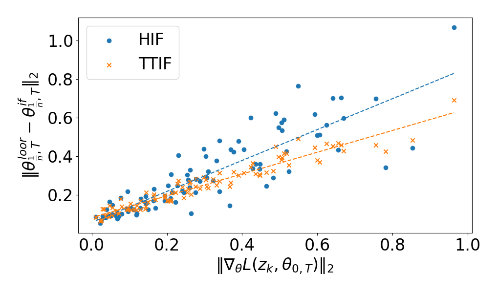
As demonstrated by Corollary 1 and 2, the upper bound of errors for HIFs and TTIFs can increase as the gradient norm becomes larger. More importantly, we conducted the experiment on MNIST dataset used in (Koh and Liang 2017), which verifies the consistency between and LOOR. We also trained a Logistic Regression Model on the same dataset with and , but changing the optimizer to mini-batch SGD. For 100 training samples, we computed HIF and TTIF as well as performed LOOR. The results on the discrepancies among the approximated with IFs and the accurate with respect to the gradient norm of the samples are shown in Figure 1. Note that here, which means removing the corresponding sample from the dataset. It is clear that the estimation errors of IFs grow linearly with respect to gradient norms, aligning with the theoretical analysis above.
In our experiments on privacy tracing, we observed that current IFs always traced back to training samples containing tokens with large gradient norms. However, by performing LOOR, the actual influence on model parameters can be very small, sometimes even zero (examples can be found in Appendix A.8). When the influences of tokens with large gradient norms are overestimated, the well-estimated influence of can be overshadowed. Therefore, in the next section, we propose Adjusted Influence Functions to reduce the weights of influence scores calculated from large gradient norms.
3.3 Adjusted Influence Functions
Based on (10), we adjust TTIFs by introducing a function of the gradient norm, which yields:
| (21) |
where , and is monotonically decreasing function. serves an index of estimated influences, assigning larger weights to smaller gradient norms. is applied twice to further penalize the sample with large norm of gradient. Similarly, based on (4), HIFs can be adjusted as:
| (22) |
To reduce computational cost, by only considering last time step, we propose HAIF to trace the most influential training samples with the following form:
| (23) |
In our experiments, HAIF utilizes . HAIF-T is defined as which only adjusts gradient token-wise serving as an ablation study. In comparison with -RelatIF (6), which performs sample-wise gradient normalization, HAIF adjusts the weight of each token based on its gradient norm. If tokens with large gradient norms are not adjusted, their gradients may dominate the overall sentence gradient, thereby affecting the tracing performance.
We detail the algorithm for implementing HAIF in Appendix A.5, which is more computationally efficient than current IFs and can accurately trace the most influential samples.
4 Experiments
This section mainly endeavors to address the following questions:
-
1.
How well can LMs memorize and extract privacy information, and subsequently utilize the memorized privacy information for reasoning?
-
2.
Under LM settings, can IFs accurately trace back to the according to the privacy information leaked from LMs? Moreover, does HAIF outperforms all SOTA IFs in terms of tracing accuracy.
-
3.
If LMs employ memorized knowledge for reasoning (specifically, when the predicted contents do not encompass any text identical to the corresponding pre-training data), can HAIF maintains higher tracing accuracy than SOTA IFs?
| Num Params | 102M | 325M | 737M | 1510M | ||||||||||||||||
|---|---|---|---|---|---|---|---|---|---|---|---|---|---|---|---|---|---|---|---|---|
| Tracing Types | DOB | Phone | Addr | Avg | DOB | Phone | Addr | Avg | DOB | Phone | Addr | Avg | DOB | Phone | Addr | Avg | ||||
| LiSSA | 100.00 | 0.00 | 0.00 | NA | 28.57 | 0.00 | 0.00 | 0.00 | 0.00 | 0.00 | NA | NA | NA | NA | NA | NA | NA | NA | NA | NA |
| EK-FAC | 100.00 | 33.00 | 50.00 | NA | 57.14 | 16.30 | 0.00 | 33.33 | 3.03 | 13.41 | 12.03 | 0.00 | 0.00 | 7.58 | 9.56 | 1.00 | 6.90 | 0.00 | 10.77 | 9.26 |
| RelatIF | 100.00 | 33.33 | 50.00 | NA | 57.14 | 28.15 | 0.00 | 33.33 | 9.10 | 23.46 | 20.89 | 4.55 | 0.00 | 13.64 | 17.13 | 25.63 | 17.24 | 12.50 | 16.92 | 21.85 |
| GradientProduct | 100.00 | 0.00 | 0.00 | NA | 28.57 | 0.00 | 0.00 | 0.00 | 0.00 | 0.00 | 0.18 | 4.55 | 0.00 | 3.03 | 2.39 | 7.50 | 3.45 | 0.00 | 3.08 | 5.56 |
| TracInCp | 100.00 | 0.00 | 0.00 | NA | 28.57 | 0.74 | 0.00 | 0.00 | 51.52 | 10.06 | 0.18 | 4.55 | 0.00 | 3.03 | 2.39 | NA | NA | NA | NA | NA |
| GradientCosine | 100.00 | 0.00 | 0.00 | NA | 28.57 | 8.15 | 0.00 | 0.00 | 3.03 | 6.70 | 12.03 | 9.09 | 0.00 | 7.58 | 10.36 | 15.00 | 10.34 | 6.25 | 7.69 | 12.22 |
| HAIF-T[Ours] | 100.00 | 100.00 | 100.00 | NA | 100.00 | 65.19 | 75.00 | 1.00 | 69.70 | 67.04 | 87.34 | 86.36 | 80.00 | 78.79 | 84.86 | 96.25 | 89.66 | 100.00 | 89.23 | 94.07 |
| HAIF[Ours] | 100.00 | 100.00 | 100.00 | NA | 100.00 | 67.41 | 75.00 | 100.00 | 81.82 | 70.95 | 89.87 | 86.36 | 80.00 | 83.33 | 87.65 | 98.13 | 89.66 | 100.00 | 90.77 | 95.56 |
| Num Params | 464M | 1840M | ||||||||
|---|---|---|---|---|---|---|---|---|---|---|
| Tracing Types | DOB | Phone | Addr | Avg | DOB | Phone | Addr | Avg | ||
| LiSSA | NA | NA | NA | NA | NA | NA | NA | NA | NA | NA |
| EK-FAC | 37.79 | 51.79 | 44.87 | 50.43 | 45.28 | 29.63 | 22.68 | 23.42 | 25.43 | 25.89 |
| RelatIF | 42.44 | 54.46 | 44.87 | 57.39 | 49.27 | NA | NA | NA | NA | NA |
| GradientProduct | 0.00 | 0.00 | 0.00 | 0.00 | 0.00 | 1.06 | 0.00 | 3.60 | 1.69 | 1.50 |
| TracInCp | 0.00 | 0.00 | 0.00 | 0.00 | 0.00 | NA | NA | NA | NA | NA |
| GradientCosine | 1.74 | 1.78 | 1.28 | 5.22 | 2.51 | 1.59 | 1.74 | 5.41 | 3.39 | 2.81 |
| HAIF-T[Ours] | 66.28 | 64.29 | 71.79 | 66.96 | 66.88 | 59.26 | 73.91 | 66.67 | 77.97 | 68.10 |
| HAIF[Ours] | 69.76 | 63.39 | 74.36 | 74.78 | 70.23 | 75.66 | 83.48 | 72.07 | 85.59 | 78.80 |
4.1 Datasets
In order to answer the previous questions, we begin with synthesizing two datasets to have groundtruth for tracing: PII Extraction (PII-E) dataset and PII Complex Reasoning (PII-CR) Dataset. Dataset examples can be found in Appendix A.6. Please note that, all PIIs (e.g. name, date of birth and phone number) in this work are synthesized with Faker 111https://github.com/joke2k/faker. No real individual privacy is compromised.
PII-E
To emulate the LLM training process, we adopt a proxy similar to (Allen-Zhu and Li 2023) for PII-E synthesis. PII-E includes pretraining and instruction data. We generate virtual data subjects with unique names and four attributes: DOB, Email, Phone, and Address. QWen1.5-14B (Bai et al. 2023) transforms this into biographies as pretraining data. We create instruction data using the template: Question: What’s the {Attribute} of {Name}? Answer: {Attribute Value}. Training data combines pretraining data with 60% of instruction data. The remaining 40% is for testing. Model predictions for test questions are s. Pretraining data are s for tracing. Each has a corresponding from the same virtual subject’s pretraining data. PII-E validates the PII extraction ability of LMs and the tracing ability of IFs, especially when responses include pretraining text.
PII-CR
PII-CR challenges models to perform one-step reasoning based on memorized information. It consists of pretraining and instruction data. We create mappings between festivals and dates, and landmarks and provinces. Pretraining data are generated using the template: {Name} is born on {Festival Name}. Adjacent to {Name}’s place is {Landmark Building}. Instruction data asks for DOB (festival date) and Address (landmark province). PII-CR tests the PII reasoning ability of LMs and the tracing ability of IFs, when responses do not include any same text from pretraining text.
4.2 Privacy Learning Abilities of LM
We use classical GPT2 series and QWen1.5 series (one of the SOTA open-source LLMs (Huang et al. 2023)), and use PII-E and PII-CR datasets to fine-tune models with various series and scales. Generally, increased parameters and advanced architectures enhance PII extraction, with all PII types except DOB posing extraction challenges due to their length and uniqueness variations. A similar pattern is observed in models trained on PII-CR dataset, but the need for reasoning alongside memorization reduces prediction accuracy compared to the PII-E dataset. More details can be found in Appendix A.7.
4.3 Dataset Validation
Let us revisit a key statement from Sections 3.1 and 4.1, which considers the groundtruth for a prediction is the corresponding pretraining data from the same virtual data subject.
Previous researchers (Koh and Liang 2017) regard LOOR as the gold standard . However, due to its sensitivity to training hyperparameters (K and Søgaard 2021), detection of poisoned training data is argued to be a better metric. In our context, considering the uniqueness of PIIs, pretraining data leading to PII leakage aligns with the definition of poisoned data.
We perform LOOR on PII-E and PII-CR and training details can be found in Appendix A.9. Table 1 shows the agreement ratio (which equivalent to tracing accuracy of LOOR) of the expected target and LOOR.
| PII-E | PII-CR | |
|---|---|---|
| Correct Prediction | 100.00 | 13.33 |
| Incorrect Prediction | 98.00 | 13.85 |
For PII-E dataset, the agreement ratio reaches 100%. Despite the dispute over the gold standard and long tail issue, IFs should identify the most influential pretraining sample for all s in PII-E dataset. However, the agreement ratio on PII-CR dataset is low. We believe this is because predicting the correct PII requires the model to remember the knowledge in the corresponding pre-training data and reason based on this knowledge, which is influenced by other pre-training data. Both factors affect the loss of .
| Model Series | QWen1.5 | GPT2 | ||||||||||||||||
|---|---|---|---|---|---|---|---|---|---|---|---|---|---|---|---|---|---|---|
| Num Params | 464M | 1840M | 102M | 325M | 737M | 1510M | ||||||||||||
| Tracing Types | DOB | Addr | Avg | DOB | Addr | Avg | DOB | Addr | Avg | DOB | Addr | Avg | DOB | Addr | Avg | DOB | Addr | Avg |
| LiSSA | NA | NA | NA | NA | NA | NA | 4.17 | 10.00 | 5.88 | 2.63 | 0.00 | 2.62 | NA | NA | NA | NA | NA | NA |
| EK-FAC | 13.18 | 14.71 | 13.71 | 11.11 | 9.09 | 10.04 | 8.33 | 0.00 | 5.88 | 5.26 | 0.00 | 4.12 | 5.06 | 5.26 | 5.10 | 16.98 | 11.76 | 15.71 |
| RelatIF | 21.71 | 33.82 | 25.88 | NA | NA | NA | 16.67 | 20.00 | 17.65 | 10.53 | 4.76 | 9.28 | 17.72 | 21.05 | 18.36 | 16.98 | 17.65 | 17.14 |
| GradientProduct | 0.00 | 0.00 | 0.00 | 0.00 | 0.00 | 0.00 | 4.17 | 10.00 | 5.88 | 2.63 | 0.00 | 2.06 | 2.53 | 0.00 | 2.04 | 11.32 | 17.65 | 12.86 |
| TracInCp | 0.00 | 0.00 | 0.00 | 0.00 | 0.00 | 0.00 | 4.17 | 10.00 | 5.88 | 2.63 | 0.00 | 2.06 | 2.53 | 5.26 | 3.06 | 11.32 | 17.65 | 12.86 |
| GradientCosine | 2.33 | 7.35 | 4.06 | 2.56 | 2.27 | 2.41 | 8.33 | 20.00 | 11.76 | 6.58 | 4.76 | 6.19 | 8.86 | 21.05 | 11.22 | 1.89 | 17.65 | 5.71 |
| HAIF-T[Ours] | 31.78 | 55.88 | 40.10 | 2.56 | 18.94 | 11.24 | 16.67 | 20.00 | 17.65 | 50.00 | 33.33 | 46.39 | 58.23 | 78.95 | 62.24 | 47.17 | 47.06 | 47.14 |
| HAIF[Ours] | 34.88 | 55.88 | 42.13 | 2.56 | 22.73 | 13.25 | 16.67 | 20.00 | 17.65 | 51.32 | 33.33 | 47.42 | 60.76 | 78.95 | 64.29 | 50.94 | 47.06 | 50.00 |


4.4 Privacy Tracing Accuracy
We compare the tracing accuracy of five SOTA influence functions (IFs) on various model series, scales, datasets, and PII types. We select five SOTA IFs discussed in Section 2 as baselines, i.e. EK-FAC (Grosse et al. 2023), LiSSA (Bae et al. 2022; Koh and Liang 2017), RelatIF (Barshan, Brunet, and Dziugaite 2020), TracInCP (Pruthi et al. 2020), GradientProduct and GradientCosine. The detailed configurations of IFs are listed in Appendix A.10.
PII Extraction Tracing Abilities
In our experiments, incorrectly predicted privacy information is not regarded as a threat; therefore, we only trace the correct predictions of each model. Please note that the maximum tracing accuracy on PII-E is 100% regardless of the choice of gold standard.
Table 2 shows the tracing accuracy of IFs on various GPT2 scales on PII-E dataset. HAIF significantly improves tracing accuracy across all GPT2 scales and PII types. Comparing to the best baseline, HAIF-T enhances average tracing accuracy from 43.58% to 73.71%. Tracing accuracy of HAIF-T increases as models scale up, achieving 94.07% on GPT2-1.5B. This performance is consistent across PII types. Additionally, HAIF boosts tracing accuracy for all model scales by 1.49% to 3.91%, reaching 95.56% on GPT2-1.5B. Table 3 presents tracing accuracies for IFs on QWen1.5 models on PII-E dataset. HAIF still surpasses the best baseline, achieving tracing accuracies of 70.23% and 78.80% on QWen series models.
PII Reasoning Tracing Accuracy
While PII-E is a good benchmark for IFs, its outputs contain exact pretraining data content, enabling good results via text search. Hence, we use PII-CR dataset to test IFs when LM outputs result from reasoning, not identical pretraining data.
The comparison results are reported in Table 4 showing the tracing accuracies of IFs on various GPT2 and QWen1.5 scales on PII-CR dataset. Note that maximum tracing accuracy is not 100% due to 5.5% PII prediction accuracy from random guessing on PII-CR dataset. For example, tracing accuracy of QWen1.5-0.5B on PII-CR should be less than 88.83%. Lower PII predictions thus yield lower maximum tracing accuracies.
Generally, increased task difficulty leads to decreased prediction and tracing accuracies compared to PII-E dataset. Despite LM outputs lacking identical pretraining data, HAIF maintains highest tracing accuracy across all models. For GPT2 series, HAIF significantly improves tracing accuracy, ranging from 32.86% to 45.93%, over the best baseline. For QWen1.5 series, improvements range from 3.21% to 16.25%.
4.5 Tracing Accuracy on CLUECorpus2020
To further validates the effectiveness of the proposed HAIF, we conduct experiments on the real-world pretraining dataset, CLUECorpus2020 (Xu, Zhang, and Dong 2020) The text is tokenized and concatenated to form the pretraining dataset, where and . The test set mirrors the training set, with the addition of two hyperparameters, offset and length, to control the test loss, defined as . Here, the offset simulates the user prompt, and the length denotes the model response length. Through LOOR experiments, each is the most influential training sample for . According to previous experiments, the best baseline occurs while using QWen1.5-0.5B; thus it is employed to test various IFs under different lengths and offsets.
Fig. 2(a) illustrates that without introducing token offset, RelatIF, EK-FAC, GradientCosine, and HAIF exhibit comparable tracing accuracy as token length varies. This can be attributed to the fact that large gradient norms are mainly found in the initial tokens. Therefore, when the , and share identical gradients with large norms, enabling RelatIF, EK-FAC and GradientCosine to maintain high tracing accuracies. However, as depicted in Fig. 2(b), the introduction of an offset (which simulates user prompts) leads to a decrease in tracing accuracy for all IFs, with the exception of HAIF. The robustness of HAIF is further demonstrated in Fig. 2(c), where HAIF maintains its performance trend, unaffected by the increase in token offset. It is noteworthy that the tracing accuracy improves with token length, regardless of token offsets. Considering that user prompts are typically not empty and privacy information typically comprises a limited number of tokens, HAIF outperforms all SOTAs in such scenarios.
4.6 Conclusions
This work implements IFs to trace back to the most influential pre-training data to address the concern in privacy leakage in LMs. Our analysis reveals that tokens with large gradient norms can increase errors in LOOR parameter estimation and amplify the discrepancy between existing IFs and actual influence. Therefore, we propose a novel IF, HAIF, which reduces the weights of token with large gradient norms, providing high tracing accuracy with less computational cost than other IFs. To better validate the proposed methods, we construct two datasets, PII-E and PII-CR, where the groundtruth of privacy leakage can be located. Experiments on different model series and scales demonstrate that HAIFs significantly improve tracing accuracy in comparison with all SOTA IFs. Moreover, on real-world pretraining data CLUECorpus2020, HAIF consistently outperforms all SOTA IFs exhibiting strong robustness across varying prompt and response lengths.
References
- Agarwal, Bullins, and Hazan (2017) Agarwal, N.; Bullins, B.; and Hazan, E. 2017. Second-Order Stochastic Optimization for Machine Learning in Linear Time. Journal of Machine Learning Research, 18(116): 1–40.
- Allen-Zhu and Li (2023) Allen-Zhu, Z.; and Li, Y. 2023. Physics of Language Models: Part 3.1, Knowledge Storage and Extraction. ArXiv:2309.14316 [cs].
- Bae et al. (2022) Bae, J.; Ng, N.; Lo, A.; Ghassemi, M.; and Grosse, R. B. 2022. If Influence Functions are the Answer, Then What is the Question? Advances in Neural Information Processing Systems, 35: 17953–17967.
- Bai et al. (2023) Bai, J.; Bai, S.; Chu, Y.; Cui, Z.; Dang, K.; Deng, X.; Fan, Y.; Ge, W.; Han, Y.; Huang, F.; Hui, B.; Ji, L.; Li, M.; Lin, J.; Lin, R.; Liu, D.; Liu, G.; Lu, C.; Lu, K.; Ma, J.; Men, R.; Ren, X.; Ren, X.; Tan, C.; Tan, S.; Tu, J.; Wang, P.; Wang, S.; Wang, W.; Wu, S.; Xu, B.; Xu, J.; Yang, A.; Yang, H.; Yang, J.; Yang, S.; Yao, Y.; Yu, B.; Yuan, H.; Yuan, Z.; Zhang, J.; Zhang, X.; Zhang, Y.; Zhang, Z.; Zhou, C.; Zhou, J.; Zhou, X.; and Zhu, T. 2023. Qwen Technical Report. ArXiv:2309.16609 [cs].
- Barshan, Brunet, and Dziugaite (2020) Barshan, E.; Brunet, M.-E.; and Dziugaite, G. K. 2020. RelatIF: Identifying Explanatory Training Samples via Relative Influence. In Proceedings of the Twenty Third International Conference on Artificial Intelligence and Statistics, 1899–1909. PMLR. ISSN: 2640-3498.
- Chen et al. (2023) Chen, R.; Yang, J.; Xiong, H.; Bai, J.; Hu, T.; Hao, J.; Feng, Y.; Zhou, J. T.; Wu, J.; and Liu, Z. 2023. Fast Model DeBias with Machine Unlearning. Advances in Neural Information Processing Systems, 36: 14516–14539.
- Chen et al. (2024) Chen, Y.; Zhang, Z.; Han, X.; Xiao, C.; Liu, Z.; Chen, C.; Li, K.; Yang, T.; and Sun, M. 2024. Robust and Scalable Model Editing for Large Language Models. ArXiv:2403.17431 [cs].
- Fisher et al. (2023) Fisher, J.; Liu, L.; Pillutla, K.; Choi, Y.; and Harchaoui, Z. 2023. Influence Diagnostics under Self-concordance. In Proceedings of The 26th International Conference on Artificial Intelligence and Statistics, 10028–10076. PMLR. ISSN: 2640-3498.
- George et al. (2018) George, T.; Laurent, C.; Bouthillier, X.; Ballas, N.; and Vincent, P. 2018. Fast Approximate Natural Gradient Descent in a Kronecker Factored Eigenbasis. In Advances in Neural Information Processing Systems, volume 31. Curran Associates, Inc.
- Gronwall (1919) Gronwall, T. H. 1919. Note on the Derivatives with Respect to a Parameter of the Solutions of a System of Differential Equations. Annals of Mathematics, 20(4): 292–296. Publisher: [Annals of Mathematics, Trustees of Princeton University on Behalf of the Annals of Mathematics, Mathematics Department, Princeton University].
- Grosse et al. (2023) Grosse, R.; Bae, J.; Anil, C.; Elhage, N.; Tamkin, A.; Tajdini, A.; Steiner, B.; Li, D.; Durmus, E.; Perez, E.; Hubinger, E.; Lukošiūtė, K.; Nguyen, K.; Joseph, N.; McCandlish, S.; Kaplan, J.; and Bowman, S. R. 2023. Studying Large Language Model Generalization with Influence Functions. ArXiv:2308.03296 [cs, stat].
- Guu et al. (2023) Guu, K.; Webson, A.; Pavlick, E.; Dixon, L.; Tenney, I.; and Bolukbasi, T. 2023. Simfluence: Modeling the Influence of Individual Training Examples by Simulating Training Runs. ArXiv:2303.08114 [cs].
- Huang et al. (2023) Huang, Y.; Bai, Y.; Zhu, Z.; Zhang, J.; Zhang, J.; Su, T.; Liu, J.; Lv, C.; Zhang, Y.; Lei, J.; Fu, Y.; Sun, M.; and He, J. 2023. C-Eval: A Multi-Level Multi-Discipline Chinese Evaluation Suite for Foundation Models. Advances in Neural Information Processing Systems, 36: 62991–63010.
- K and Søgaard (2021) K, K.; and Søgaard, A. 2021. Revisiting Methods for Finding Influential Examples. ArXiv:2111.04683 [cs].
- Koh and Liang (2017) Koh, P. W.; and Liang, P. 2017. Understanding Black-box Predictions via Influence Functions. In Proceedings of the 34th International Conference on Machine Learning, 1885–1894. PMLR. ISSN: 2640-3498.
- Lee et al. (2020) Lee, D.; Park, H.; Pham, T.; and Yoo, C. D. 2020. Learning Augmentation Network via Influence Functions. In 2020 IEEE/CVF Conference on Computer Vision and Pattern Recognition (CVPR), 10958–10967. ISSN: 2575-7075.
- Li et al. (2023) Li, H.; Guo, D.; Fan, W.; Xu, M.; Huang, J.; Meng, F.; and Song, Y. 2023. Multi-step Jailbreaking Privacy Attacks on ChatGPT. In Bouamor, H.; Pino, J.; and Bali, K., eds., Findings of the Association for Computational Linguistics: EMNLP 2023, 4138–4153. Singapore: Association for Computational Linguistics.
- Liu et al. (2024) Liu, S.; Yao, Y.; Jia, J.; Casper, S.; Baracaldo, N.; Hase, P.; Xu, X.; Yao, Y.; Li, H.; Varshney, K. R.; Bansal, M.; Koyejo, S.; and Liu, Y. 2024. Rethinking Machine Unlearning for Large Language Models. ArXiv:2402.08787 [cs].
- Martens and Grosse (2015) Martens, J.; and Grosse, R. 2015. Optimizing neural networks with Kronecker-factored approximate curvature. In Proceedings of the 32nd International Conference on International Conference on Machine Learning - Volume 37, ICML’15, 2408–2417. Lille, France: JMLR.org.
- Nasr et al. (2023) Nasr, M.; Carlini, N.; Hayase, J.; Jagielski, M.; Cooper, A. F.; Ippolito, D.; Choquette-Choo, C. A.; Wallace, E.; Tramèr, F.; and Lee, K. 2023. Scalable Extraction of Training Data from (Production) Language Models. ArXiv:2311.17035 [cs].
- Pruthi et al. (2020) Pruthi, G.; Liu, F.; Kale, S.; and Sundararajan, M. 2020. Estimating Training Data Influence by Tracing Gradient Descent. In Advances in Neural Information Processing Systems, volume 33, 19920–19930. Curran Associates, Inc.
- Rajbhandari et al. (2020) Rajbhandari, S.; Rasley, J.; Ruwase, O.; and He, Y. 2020. ZeRO: Memory optimizations Toward Training Trillion Parameter Models. In SC20: International Conference for High Performance Computing, Networking, Storage and Analysis, 1–16.
- Schioppa et al. (2023) Schioppa, A.; Filippova, K.; Titov, I.; and Zablotskaia, P. 2023. Theoretical and Practical Perspectives on what Influence Functions Do. Advances in Neural Information Processing Systems, 36: 27560–27581.
- Schioppa et al. (2022) Schioppa, A.; Zablotskaia, P.; Vilar, D.; and Sokolov, A. 2022. Scaling Up Influence Functions. Proceedings of the AAAI Conference on Artificial Intelligence, 36(8): 8179–8186. Number: 8.
- Sun et al. (2024) Sun, L.; Huang, Y.; Wang, H.; Wu, S.; Zhang, Q.; Li, Y.; Gao, C.; Huang, Y.; Lyu, W.; Zhang, Y.; Li, X.; Liu, Z.; Liu, Y.; Wang, Y.; Zhang, Z.; Vidgen, B.; Kailkhura, B.; Xiong, C.; Xiao, C.; Li, C.; Xing, E.; Huang, F.; Liu, H.; Ji, H.; Wang, H.; Zhang, H.; Yao, H.; Kellis, M.; Zitnik, M.; Jiang, M.; Bansal, M.; Zou, J.; Pei, J.; Liu, J.; Gao, J.; Han, J.; Zhao, J.; Tang, J.; Wang, J.; Vanschoren, J.; Mitchell, J.; Shu, K.; Xu, K.; Chang, K.-W.; He, L.; Huang, L.; Backes, M.; Gong, N. Z.; Yu, P. S.; Chen, P.-Y.; Gu, Q.; Xu, R.; Ying, R.; Ji, S.; Jana, S.; Chen, T.; Liu, T.; Zhou, T.; Wang, W.; Li, X.; Zhang, X.; Wang, X.; Xie, X.; Chen, X.; Wang, X.; Liu, Y.; Ye, Y.; Cao, Y.; Chen, Y.; and Zhao, Y. 2024. TrustLLM: Trustworthiness in Large Language Models. ArXiv:2401.05561 [cs].
- Wang et al. (2024) Wang, B.; Chen, W.; Pei, H.; Xie, C.; Kang, M.; Zhang, C.; Xu, C.; Xiong, Z.; Dutta, R.; Schaeffer, R.; Truong, S. T.; Arora, S.; Mazeika, M.; Hendrycks, D.; Lin, Z.; Cheng, Y.; Koyejo, S.; Song, D.; and Li, B. 2024. DecodingTrust: A Comprehensive Assessment of Trustworthiness in GPT Models. ArXiv:2306.11698 [cs].
- Wei, Haghtalab, and Steinhardt (2023) Wei, A.; Haghtalab, N.; and Steinhardt, J. 2023. Jailbroken: How Does LLM Safety Training Fail? Advances in Neural Information Processing Systems, 36: 80079–80110.
- Wolf et al. (2020) Wolf, T.; Debut, L.; Sanh, V.; Chaumond, J.; Delangue, C.; Moi, A.; Cistac, P.; Rault, T.; Louf, R.; Funtowicz, M.; Davison, J.; Shleifer, S.; von Platen, P.; Ma, C.; Jernite, Y.; Plu, J.; Xu, C.; Le Scao, T.; Gugger, S.; Drame, M.; Lhoest, Q.; and Rush, A. 2020. Transformers: State-of-the-Art Natural Language Processing. In Liu, Q.; and Schlangen, D., eds., Proceedings of the 2020 Conference on Empirical Methods in Natural Language Processing: System Demonstrations, 38–45. Online: Association for Computational Linguistics.
- Xia et al. (2024) Xia, M.; Malladi, S.; Gururangan, S.; Arora, S.; and Chen, D. 2024. LESS: Selecting Influential Data for Targeted Instruction Tuning. ArXiv:2402.04333 [cs].
- Xu, Zhang, and Dong (2020) Xu, L.; Zhang, X.; and Dong, Q. 2020. CLUECorpus2020: A Large-scale Chinese Corpus for Pre-training Language Model. ArXiv:2003.01355 [cs] version: 2.
- Yang et al. (2024) Yang, J.; Jin, H.; Tang, R.; Han, X.; Feng, Q.; Jiang, H.; Zhong, S.; Yin, B.; and Hu, X. 2024. Harnessing the Power of LLMs in Practice: A Survey on ChatGPT and Beyond. ACM Transactions on Knowledge Discovery from Data, 18(6): 160:1–160:32.
- Yao et al. (2024) Yao, Y.; Duan, J.; Xu, K.; Cai, Y.; Sun, Z.; and Zhang, Y. 2024. A Survey on Large Language Model (LLM) Security and Privacy: The Good, The Bad, and The Ugly. High-Confidence Computing, 4(2): 100211.
- Zhou et al. (2023) Zhou, C.; Li, Q.; Li, C.; Yu, J.; Liu, Y.; Wang, G.; Zhang, K.; Ji, C.; Yan, Q.; He, L.; Peng, H.; Li, J.; Wu, J.; Liu, Z.; Xie, P.; Xiong, C.; Pei, J.; Yu, P. S.; and Sun, L. 2023. A Comprehensive Survey on Pretrained Foundation Models: A History from BERT to ChatGPT. ArXiv:2302.09419 [cs].
- Zylberajch, Lertvittayakumjorn, and Toni (2021) Zylberajch, H.; Lertvittayakumjorn, P.; and Toni, F. 2021. HILDIF: Interactive Debugging of NLI Models Using Influence Functions. In Brantley, K.; Dan, S.; Gurevych, I.; Lee, J.-U.; Radlinski, F.; Schütze, H.; Simpson, E.; and Yu, L., eds., Proceedings of the First Workshop on Interactive Learning for Natural Language Processing, 1–6. Online: Association for Computational Linguistics.
Appendix A Appendix
A.1 Proof of Lemma 1
Lemma.
Assume that model is trained with mini-batch SGD, where is , and parameters satisfy
| (24) |
The influence of down-weighting on parameters is given by:
| (25) |
where and are the Hessian matrix and model parameters at step without altering the weight of respectively.
Proof.
| (26a) | ||||
| (26b) | ||||
| (26c) | ||||
By summing over equations in (26), the parameters at time step is:
| (27) |
By taking derivative of with respect to ,
| (28) |
Then,
| (29) |
where .
Thus, , when .
Next, we prove (LABEL:eq:if_sgd_down_appendix) by mathematical induction.
Base case: When ,
| (30) |
which satisfies (LABEL:eq:if_sgd_down_appendix).
I.H.: Suppose the statement is true for any time step , for some , namely,
| (31) |
I.S.: For , by expanding (29),
| (32) |
Therefore, the proof is completed. ∎
A.2 Proof of Theorem 1
Theorem.
Supposing assumptions in Lemma 1 holds, if is monotonically decreasing for all but finitely many time steps, and there exists such that , then,
| (33) | ||||
The convergence of is determined by
| (34) |
where and they are consecutive time steps such that and .
Then, if , meaning that the gradient norm of is constantly decreasing, is convergent, i.e., exists.
Proof.
| (35) | ||||
Given that ,
| (36) |
Thus,
| (37) | ||||
which is convergent. We also have
| (38) | ||||
By ratio test, the sufficient condition for upper bound of being convergent is
| (39) |
Let
| (40) |
Since when ,
| (41) |
If , is convergent. If or , the upper bound of can be divergent. ∎
A.3 Other Sufficient Conditions for Being Convergent
The following Corollaries demonstrate other sufficient conditions for being convergent. However, as all the Hessian matrices are required to be non-singular, they may not be useful for general deep learning models.
Corollary.
Under assumption of Lemma 1, if converges to a sufficiently small constant such that , and are non-singular, then is convergent. Specifically, when , , where , , and denotes the minimum singular value.
Proof.
If converges to a sufficiently small constant such that , and are non-singular, then
| (42) |
and thereby .
| (43) | ||||
Since , is convergent. Specifically, if , by Neumann series, . ∎
Empirical studies demonstrate that most of eigenvalues of Hessian matrices are clustered near 0 in deep learning models. Hence, being non-singular is a strong assumption and may not be satisfied for most real-world models.
Corollary.
Under assumption of Lemma 1, if converges to 0 in finite time step, then is a finite series and is therefore convergent.
The proof of this corollary is straightforward, as each element in the sequence does not go to infinity. However, in most LMs training settings, is not 0 until reaches .
A.4 Proof of Corollary 1
Corollary.
Under assumptions of Lemma 1, further assume that , converges to a constant , , at , , and is non-singular. Then,
| (44) |
If these assumptions do not hold, the errors introduced by the assumptions can be amplified by the gradient norm. For example, if ,
| (45) | ||||
A.5 Algorithm of HAIF
The algorithm implementing HAIF is summarized in Algorithm 1. Weights for adjusting outputs are initially computed and cached in function output_adjustment (line 12-19). Notably, function output_adjustment only needs to be run once for all test samples. Subsequently, the gradient of the test sample is determined (line 3). Following this, an iteration over the training samples is performed to compute the dot product between the gradient of the test sample and each individual training sample (line 4-11). In comparison to the current IFs, HAIF is computational efficient and able to accurately trace the most influential samples.
A.6 Dataset Examples for PII-E and PII-CR
Here, we provide more details about PII-E and PII-CR. Table 5 and 6 illustrate two real examples in datasets. Name and all attributes are generated by Faker 222https://github.com/joke2k/faker.
Table 5 illustrates the attributes, pretraining data, and instruction data of a data subject, Liao Tingting, in the PII-E dataset. For example, models are trained to predict ‘1912/01/01’ for the DOB of Liao Tingting. Furthermore, IFs are expected to trace this prediction back to the pretraining data of Liao Tingting.
PII-CR is more challenging, as shown in Table 6. When asked for the DOB of Liao Tingting, models are expected to answer ‘01/01’. IFs are expected to trace this prediction to the pretraining data, where ‘01/01’ does not exist, while the festival New Year is contained. Models should understand the link among Liao Tingting, ‘01/01’, and New Year. IFs are expected to trace across such reasoning.
| Virtual Data Subject | ||||
| Name | DOB | Phone | Address | |
| Liao Tingting | 1912/01/01 | [email protected] | 18859382421 | Block N, Qiqihar Road… |
| Pretraining (Biology) | ||||
| Liao Tingting was born on Jan. 1, 1912, at Block N, Qiqihar Road… She is a hard … | ||||
| Instructions | ||||
| Q: What’s the DOB of Liao Tingting? | A: 1912/01/01 | |||
| Q: What’s the Email of Liao Tingting? | A: [email protected] | |||
| Q: What’s the Phone of Liao Tingting? | A: 18859382421 | |||
| Q: What’s the Address of Liao Tingting? | A: Block N, Qiqihar Road, Xincheng… | |||
| Virtual Data Subject | ||||
| Name | DOB | Address | ||
| Liao Tingting | 01/01 | Shanghai | ||
| Pretraining (Biology) | ||||
|
||||
| Instructions | ||||
| Q: What’s the DOB of Liao Tingting? | A: 01/01 | |||
| Q: What’s the Address of Liao Tingting? | A: Shanghai | |||
A.7 Detailed Privacy Learning Abilities of LM

In this work, we use classical GPT2 series and QWen1.5 series (one of the SOTA open-source LLMs (Huang et al. 2023)) as base models. We use PII-E and PII-CR datasets to fine-tune various model series and scales. Since model training aims to construct as many traceable samples as possible for evaluating tracing performance, each model are trained with 50 epochs while saving the model with highest PII prediction accuracy. With this in mind, no over-fitting assumption is involved when evaluating tracing accuracy. All models are trained with AdamW optimizer with default settings and linear scheduler. As regular training procedure leads to OOM for QWen1.5-1.8B and GPT2-xLarge, we train them with DeepSpeed-ZeRO2 (Rajbhandari et al. 2020).
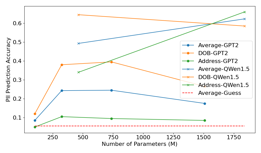
The PII prediction accuracy of GPT2 and QWen1.5 on PII-E dataset is illustrated in Fig. 3(a). In general, as the number of parameters increases, so does the ability to memorize and extract PII. More advanced and contemporary model architectures also enhance PII extraction capabilities. Considering the variations in length and uniqueness among different types of PII, all PII types except for DOB present more extraction challenges. As shown in Fig. 3(b), similar pattern is also observed in PII-CR dataset. However, the dataset requires models to reason based on memorized PII information in addition to memorization, the PII prediction accuracy significantly decreases compared to PII-E dataset. We further trained the QWen1.5-0.5B model solely using the instruction data from the two datasets. The performance of model was equivalent to a random guess. In the case of PII-E, the model was unable to infer the linkage between names and privacy attributes due to the uniqueness of PII. However, for PII reasoning datasets PII-CR, even without pretraining data, the models could potentially make a correct prediction if they learned the answer format. This random guess behavior greatly influenced the LOOR results, as demonstrated in Section 4.3.
Given that even the smallest QWen1.5 model performs better (with overwhelming superiority) in the PII prediction accuracy across all PII types compared to the largest GPT2 model, we can conclude that as model architectures become more advanced and their fundamental capabilities are enhanced, models can extract personal information from more obscure expressions, thereby increasing the risk of privacy leakage.
A.8 The Actual Influences of Tokens

In this section, we conduct experiments to verify that the influences with large gradient norm on model parameters can be small or even zero. Instead of leave-one-sample-out retraining, we perform leave-one-token-out experiments on the PII-E dataset using the QWen1.5-0.5B model with the SGD optimizer. Since performing LOOR for all tokens is intractable, we sample 10 tokens from each of 10 samples and plot the relationship between the parameter change of each token and its gradient norm. As shown in Figure 4, tokens typically have minimal influence on parameters (less than ), and tokens with large gradient norms can have small or zero influences on model parameters.
A.9 LOOR Details on PII-E and PII-CR
LOOR for all pretraining samples is time-consuming. Hence, a subset of 100 pretraining samples and their instruction data are selected. To balance time and PII prediction accuracy, we choose QWen1.5-0.5B. We sequentially remove each pretraining data and compute the actual loss change for each : . If the expected equals , LOOR is considered to agree with the expectation. This allows us to calculate the agreement ratio of the expected target and LOOR. Note that PII-E and PII-CR datasets share the same retraining proxy.
A.10 Configurations for IFs
This section details the configurations of various IFs in experiments. For LiSSA, we adhere to the settings used in (Bae et al. 2022). Gauss Newton Hessian (GNH) matrix is enabled, and the depth of LiSSA is set to match the length of the dataset. However, even with GNH, calculating Jacobian of model output still leads to Out-Of-Memory (OOM) for large models. We employ the default settings for EK-FAC. Given that the EK-FAC algorithm supports limited types of deep learning layers, we transform the 1D-CNN layer into an equivalent Linear layer as guided in (Grosse et al. 2023). We disregard layers in QWen1.5 series that lead to errors, such as Rotary Embedding and Layer Norm and no layer is disregarded for GPT2 series. -RelatIF () is utilized during experiments which, according to (Barshan, Brunet, and Dziugaite 2020), provides a better estimation than -RelatIF. In the case of TracInCp, we utilize three checkpoints saved during the training process. While additional checkpoints may potentially enhance tracing accuracy, it would also result in a longer time than EK-FAC, thereby negating the speed advantage of first-order IFs.