Traces on General Sets in for Functions with no Differentiability Requirements††thanks: The author’s research is supported by the NSF award DMS-1716790
Abstract
This paper is concerned with developing a theory of traces for functions that are integrable but need not possess any differentiability within their domain. Moreover, the domain can have an irregular boundary with cusp-like features and codimension not necessarily equal to one, or even an integer. Given and , we introduce a function space for which a well-defined trace operator can be identified. Membership in constrains the oscillations in the function values as is approached, but does not imply any regularity away from . Under connectivity assumptions between and , we produce a linear trace operator from to the space of measurable functions on . The connectivity assumptions are satisfied, for example, by all -sided nontangentially accessible domains. If is upper Ahlfors-regular, then the trace is a continuous operator into a Sobolev-Slobodeckij space. If and is further assumed to be lower Ahlfors-regular, then the trace exhibits the standard Lebesgue point property. To demonstrate the generality of the results, we construct with a -dimensional Ahlfors-regular satisfying the main domain hypotheses, yet is nowhere rectifiable and for every neighborhood of every , there exists a boundary point within that neighborhood that is only tangentially accessible.
Keywords:
Nonlocal function spaces, Trace operator, Higher codimensional boundaries, Ahlfors-regular boundaries
AMS2010:
35A23, 46E35, 47G10
1 Introduction
1.1 Overview
Suppose that is an open, not necessarily bounded, set and that is uniformly continuous. Though the boundary is not in the domain of , there is a natural choice for a trace function that can be identified as the values of on , since has a continuous extension to . In the context of Sobolev spaces, where is not necessarily continuous in , the well-known Gagliardo’s theorem [19] states that, with a sufficiently regular boundary, this trace operator can be extended from the space of functions with uniformly continuous derivatives to a continuous linear operator , for each . Here and is the standard Sobolev–Slobodeckij space (Definition 1.3). Generalizations to Sobolev-Slobodeckij and Besov spaces, traces on general closed subsets of , Sobolev and Besov spaces on metric spaces, Sobolev spaces with variable exponent, etc. have since been produced (see [14, 31, 33, 34, 39]). This paper is concerned with establishing analogous trace results compatible with a nonlocal framework, where only -integrability is assumed away from the boundary.
There has been a surge of interest in developing and analyzing models that employ a nonlocal operator. Such models can incorporate long-range interactions and multiple scales and can expand the space of admissible solutions to permit singular and discontinuous attributes. Nonlocal models have been successfully employed in a wide variety of contexts, including image processing [24, 32], population and flocking models [8, 40], diffusion [3], phase transitions [5, 23], and material deformation with failure in peridynamics models [41, 42]. For a comprehensive introduction to nonlocal modeling and their analysis, we refer to the monograph [15].
A common class of nonlocal operators have a convolution, or cross-correlation, like structure. At each point , the operator uses an integral and an integrable kernel to accumulate weighted data for a function over a neighborhood of . This makes them generally insensitive to function values on sets of zero measure and, in particular, to function irregularities across sets of dimension less than . With an appropriate kernel, however, the operator can approximate a differential operator and provide information about the rate of change of a function.
The current work contributes to the rigorous development of a framework in which convolution-like operators, with integrable kernels, can incorporate data on sets with positive codimension. In addition to mathematical interest, there are two primary motivations for these efforts. Both are related to the fact that at points where the support of the kernel extends outside of , the evaluation of the operator requires function values outside of . Thus, for associated nonlocal problems, the analogue of a Dirichlet-type boundary condition is a volume-constraint, where the value of a solution is prescribed on a region of positive measure in [16, 38]. It can be a nontrivial issue to identify appropriate volume-constraints when data on only a lower-dimensional set is readily available. If the integral operator is responsive to function behavior on , then one can instead formulate nonlocal problems subject to classical Dirichlet-type boundary conditions. This also facilitates seamless transitions between nonlocal and local system descriptions. There is substantially more computational expense to numerically solve nonlocal equations when compared to their local counterpart. With a nonlocal operator that “localizes” as is approached, one can couple a computationally efficient local model to a nonlocal model that confined to a region where it is essential to employ nonlocal operators [12, 43]. The set is a lower-dimensional interface between these two regions. In both contexts, it is essential to have a trace theory to ensure well-posedness and mathematical consistency.
In [44], Du and Tian produced some of the first trace results for functions in the nonlocal setting, with operators that have an integrable kernel that concentrates near the boundary. They considered the space consisting of functions satisfying , where is an open Lipschitz domain and
Here
where denotes the family of Borel subsets of , is the Lebesgue measure of , and is the open ball centered at with radius . The kernel, in the semi-norm , can be identified as . Since is uniformly positive on any open compactly contained in , one can only expect . Thus, the space includes functions that have no regularity, beyond square-integrability, away from the . As the is approached, however, the kernel concentrates sufficiently strongly that the behavior of at contributes to . In fact, the singularity is strong enough that is sensitive to oscillations in at the boundary and implies that there is a well-defined trace and, moreover, that . These results have recently been generalized to exponents in [17].
In this paper we vastly expand the class of functions and domains, for which a well-defined trace can be identified for a given . Let and be given. For each , define
| (1) |
The focus of this paper is on developing a trace theory for functions belonging to the space
A straightforward argument shows that , given by , provides a semi-norm. We easily see that if for some , we have throughout , then , with is a Besov space, as defined in [31]. Moreover, the spaces introduced in [17, 44] are subspaces of the corresponding space , with constant. (For example, .) In fact, Example 1.2 shows that, in general, the containment is strict. Thus, many results currently available in the literature can be viewed as corollaries of the trace theorems established in this paper.
With , the main results of the paper provide assumptions on , , and (collected in Section 1.3) that ensure the existence of a continuous linear trace operator , for some . The primary assumptions on and are (H1) a corkscrew-type condition, (H2) a uniform-connectedness condition, (H3) a constraint on the oscillations of near , and (H4) Ahlfors-regularity of . Loosely speaking, the oscillation constraint is satisfied if , for near . The values of depend, in an explicit way, on the approachability of from . Following some definitions recorded in Section 1.2, precise statements of the main assumptions and theorems are given in Sections 1.3 and 1.4.
The distinguishing features of this work are the following:
-
•
We provide trace results allowing “very rough” boundaries. In [17] and [44], the set is required to be Lipschitz, so that an atlas of Lipschitz transforms are available to “flatten out” . They connect the rate of change of a function in directions parallel to the flattened boundary to the rate of change in the normal direction. In this paper, a different approach is presented, based on a continuous extension of a function (3) related to the mean values of . The corkscrew and connectedness properties ensure there is a region of approach to points in that allows us to work directly with , without any transformations, and allow to have minimal regularity.
In fact, identifying a natural candidate for a measurable trace does not require any assumptions on and beyond (H1) and (H2). Assuming upper Ahlfors-regularity, we prove . If, additionally, there is a lower Ahlfors-regular neighborhood in , then we can establish the Lesbesgue point property for within that neighborhood; i.e., as , the mean values of over converge in the -norm to , for a.e. . Thus, with respect to the surface measure, agrees a.e. on with the strictly defined function associated with .
-
•
Within , the functions need only be -integrable. Given a function and an open set compactly contained in , Jensen’s inequality implies
since and is uniformly positive in . Hence, . As with the space , however, no additional regularity can be expected for in , regardless of the behavior of in . This makes a viable solution space for nonlocal systems where even discontinuous functions are admissible. For models of phenomena exhibiting sharp transitions or jumps, it is critical to include irregular functions as solution candidates. Moreover, functions in this space possess well-defined fine properties as we approach .
-
•
The traces are captured on possibly “very thin or porous” sets. The set can have non-integer Hausdorff dimension, any positive codimension, and may also possess cusp-like features. To demonstrate how irregular the domain can be, we produce an , with a nonrectifiable Ahlfors-regular self-similar set that has Hausdorff dimension and has the following property: for every and , there exists a that is only tangentially accessible. In other words, the cone of directions in the approach region for degenerates as it is approached. Nevertheless, provided the oscillation constraint is satisfied, there is a trace possessing the Lebesgue point property (see Example 1.1(b), Remark 4(b), and Section 5). We mention the recent interest in developing a theory for elliptic problems with higher-codimensional boundaries [9, 10, 21, 37] and trace theorems and boundary value problems on fractal sets [1, 2, 7].
1.2 Definitions
A more detailed presentation of the main theorems requires some additional definitions. For each , , and , define . Given and , we use to denote the -dimensional Hausdorff measure of . We use for the space of Borel-measurable functions. In general, by measurable, we mean Borel-measurable. We now introduce the two main geometric properties needed throughout the paper. A discussion of these definitions with accompanying figures is provided in the next section, following the main assumptions.
Definition 1.1.
With , we will say that is an -corkscrew region for if there exists a such that, for each , there exists satisfying
We refer to as the radius of .
Definition 1.2.
With , we will say that is -connected to if there exists with the following property: for each , there exists such that for any , if
then there exists a rectifiable path between and such that
| (2) |
In the definition above, without loss of generality, we assume , if . Next we recall the definition of the Sobolev-Slobodeckij spaces.
Definition 1.3.
Let be a -dimensional set. For each and , define by
and the Sobolev-Slobodeckij space
If is a closed set and , then our definition of corresponds to the definition of the Besov space given in [30] (see also [31]). We note that, in general, Definition 1.3 does not provide the standard Sobolev or Sobolev-Slobodeckij spaces when . In fact, if is an open connected set, , and , as defined above, then is a constant function [6, 11]. It appears to be unknown whether this is also true for not open.
Finally, we need a bit more notation. For each and , set
(See Fig. 2 below.) Given , we also define . For convenience, we define by
We note that is piecewise bilinear and that is increasing, for each . For the remainder of the paper, we fix the parameters and and the uniformly bounded measurable functions and . Put . For each , define by
We observe that the above functions are each measurable and uniformly bounded.
1.3 Assumptions
We now list our primary assumptions for , and the space . We assume that has -dimension. When convenient, we will just write and for and , respectively.
-
(H1)
Uniform -Corkscrew Condition: There exists such that, for each , the set is an -corkscrew region for with radius .
-
(H2)
Uniform -Connectedness Condition: There exists such that, for each , the set is -connected to .
-
(H3)
Oscillation Constraints:
-
(H3′)
Pointwise Oscillation Constraint at :
-
(H3′′)
Uniform Oscillation Constraint near :
-
(H3′)
-
(H4)
Ahlfors-Regularity: There exists such that, for each ,
-
(H4′)
Upper Ahlfors-Regularity:
-
(H4′′)
Lower Ahlfors-Regularity:
-
(H4′)
Example 1.1.
-
(a)
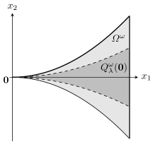
The prototypical example for is a wedge-like region where is at a cusp. Let and be given. Define
Then, for any , the hypotheses (H1) and (H2) are satisfied with and . Figure 1 depicts the approach region when .
-
(b)
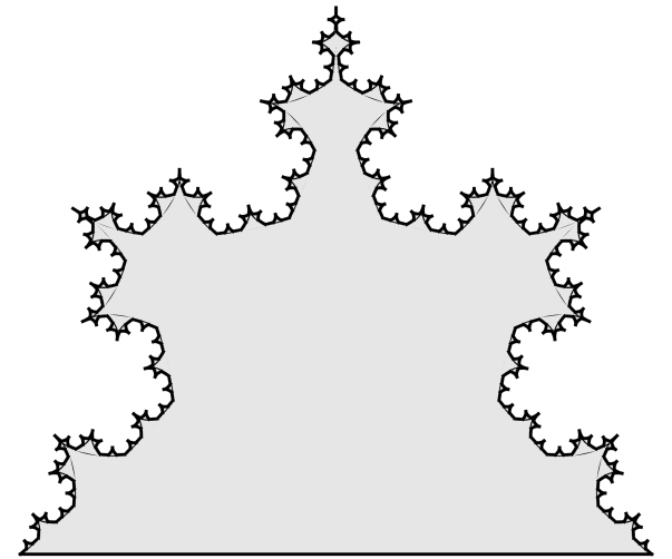
As mentioned in the introduction, assumptions (H1) and (H2), themselves, do not imply any regularity of the boundary. The Koch snowflake is a well-known example of an nontangentially accessible (NTA) domain (see Remark 1(a) and [13]) that has a nonrectifiable boundary but satisfies (H1) and (H2), with and independent of . The Koch snowflake can be generated as the union of an iteratively produced sequence of polygonal domains. The initial domain is an equilateral triangle, for example with defined in Example 1.1(a) above. Subsequent domains are obtained by replacing the middle third of the boundary line segments with an appropriately scaled outward-pointing equilateral triangle. With a similar procedure, using with , we can produce a “prickly” version of the snowflake domain (see Fig. 2). Taking to be the fractal portion of the resulting domain boundary, we find that its Hausdorff dimension is and . Moreover, and satisfy hypotheses (H1) and (H2), with , and both (H4′) and (H4′′). The set , however, fails to be a -sided NTA domain. More specifically, for every and , there exists such that there is no -connected -corkscrew region with positive radius for , for any and . Thus, in particular, is not a -sided NTA domain, for any . Additional details are provided in the appendix (Section 5).
We next put the corkscrew and connectedness assumptions into a broader context.
Remark 1.
Together, (H1) and (H2) ensure each point can be approached along a path with a quantitative control on the distance between points and . For the rest of this remark, suppose that is bounded and that on .
-
(a)
In this setting, hypotheses (H1) is the standard (interior) corkscrew condition. If also possesses the (interior) Harnack chain property, then is said to be a -sided NTA domain. An NTA domain is a -sided NTA domain such that also satisfies the corkscrew condition. These domains were introduced in [27] in connection to the absolute continuity of the harmonic measure with respect to the surface measure on . As indicated in Example 1.1(b), NTA domains need not even have rectifiable boundaries. Recently, it has been shown that if is -sided NTA and is both -dimensional and upper and lower Ahlfors-regular, then rectifiability of is actually equivalent to the absolute continuity of the harmonic measure [4].
-
(b)
The motivation for (H2) is Lemma 2.1 in [10]. As part of their investigation of elliptic problems in domains with higher codimensional boundaries, they show that Ahlfors-regular sets in , with dimension , satisfy (H2), again with . There is a close relation between assumptions (H1) and (H2) and local uniformity. The domain is locally uniform if there exists and such that, for every satisfying , there exists a rectifiable path between and such that
and
We see that local uniformity implies (H2) with independent of . Assumptions (H1) and (H2) together, however, imply is locally uniform (see Lemma A.1 and the proof for Theorem 2.15 in [4]). A condition equivalent to local uniformity is the -condition. It has been shown that, on -domains, there exists a linear continuous extension operator for the BMO and Sobolev mappings [28, 29]. If is locally uniform with , then it is a uniform domain. These domains were introduced in [35], for which injectivity and approximation results for locally bi-Lipschitz mappings were established. The class of uniform domains is actually equivalent to the class -sided NTA. In view of part (a) above, we see that assumptions (H1) and (H2) are both satisfied, with , by -sided NTA domains. We point out that, in Example 1.1(b), there are no locally uniform neighborhoods of any point in .
Assumptions (H3) can, in some sense, be interpreted as a requirement that the oscillations in decay as is approached. If , then there exists such that
The left-hand side “measures” the deviation of the values of from over the ball . Since , (H3) implies that, for each , there exists a such that is uniformly positive within the corkscrew region . Thus, (H3) ensures the oscillations of dampen in , as , which allows a well-defined value for to be identified.
While Jensen’s inequality implies, for all , we have
As just discussed, assumption (H3) is a type of decay requirement for the oscillations of but only in the sense of averages. This still allows the oscillations with uniformly positive amplitude to concentrate on sets of decreasing measure, and its possible for , for every .
Example 1.2.
For this example, we use and , so assumptions (H1) and (H2) are obviously satisfied. Fix and . We will construct such that , for all . Here, we are putting on . For each , define
so and . On the interval , we define and extend to by putting , for each . Since is symmetric, it is sufficient to show and , for . We observe that, for each , if , then
Consequently, . Furthermore, if , then either
In either case, . Set . Now, if , then and
On the other hand, if , then and . We conclude that
Thus,
Since and , we conclude that
Plugging in the definition for , we see that
Remark 2.
If we modify the definition of , on , to , then we find yet still , for all .
1.4 Main Results
Given , we define by
| (3) |
where . The function is continuous in . Our first result identifies the trace of on through a continuous extension of to at -a.e. point in .
Theorem 1.1.
Assume (H1) and (H2), and (H3). Then there exists a linear operator such that, for each there exists a -measurable set such that
| (4) |
Moreover, for every and , there exists a with the following property: for each there exists such that
| (5) |
Remark 3.
If , then , for all .
Assuming a stronger oscillation constraint in a neighborhood of and some regularity for , we may establish some differentiability and the Lebesgue point property for the trace operator provided by the previous theorem.
Theorem 1.2.
Assume (H1), (H2), and (H3). Put .
-
(a)
If satisfies (H4), then is a continuous linear operator, for each .
-
(b)
If satisfies both (H4) and (H4) and , for all , then
Remark 4.
-
(a)
As mentioned in Remark 1, if is a -sided NTA domain, then it satisfies (H1) and (H2), with and . Assuming is Ahlfors-regular, the hypotheses of Theorem 1.1 and both parts of Theorem 1.2 are satisfied if there exists an such that in .
-
(b)
For a concrete example, consider and as described in Example 1.1(b), with , so and assumptions (H1), (H2), and (H4) are satisfied. Suppose that, for some and constants ,
where . Theorem 1.1 and Theorem 1.2(a) require to be in a region where (shaded region in Fig. 4). For Theorem 1.2(b), we need (shaded region in Fig. 4).

Figure 3: Region where 
Figure 4: Region where (Note: Generally, the curves do not have a common point of intersection.)
-
(c)
In Section 1.1, it was mentioned that . Theorem 1.2(b) implies that, for sufficiently small , we find , for -a.e. (see Remark 8(b)). It is unclear, however, whether , even under the assumptions of Theorem 1.2(b).
1.5 Organization of Paper
In the next section, we establish some results needed for the main theorems. Lemma 2.6, in particular, provides the key bounds for the rate of change for within an approach region . The main result in Section 3 is Theorem 3.1, which is a slight refinement of Theorem 1.1. As a corollary, we also show that the Lebesgue point property holds for the trace when the means are taking over . Both parts of Theorem 1.2 follow from the main results in Section 4. Part (a) is a consequence of Theorem 4.5, where a more precise connection between the fractional differentiability of and certain subsets of is provided. The Lebesgue point property at points contained in a relative neighborhood of is proved in Theorem 4.6. The paper concludes with an Appendix, in Section 5, where the claims made in Example 1.1(b) are justified.
2 Supporting Results
For the remainder of the paper, fix and put . We use to denote a constant that may change from line to line but, unless otherwise indicated, is independent of the functions and and the parameters , , and . In particular, it may depend on , , , , , and .
Lemma 2.1 (Modified Giusti’s Lemma).
Suppose that is an -valued function satisfying the following:
-
(i)
The domain for includes all open sets in ;
-
(ii)
is finite, nonnegative, and nondecreasing;
-
(iii)
is countably superadditive; i.e. if are disjoint open subsets of , then
Let be given, and set
Then and .
Proof.
Recall that the -outer measure is defined by
where
| (6) |
We will use Vitali’s Covering Lemma. Let and be given. For each , we may select such that
Thus . By Vitali’s Covering Lemma, we may extract a countable sets and such that the sets , with , are mutually disjoint and
It follows that
Since was arbitrary and , we conclude that . Taking the limit, as , yields the result. ∎
Remark 5.
Our proof for Lemma 2.1 is a modification of one found, for example, in [18] (see also [25] for the original version). In [18], it is shown that the set
is a -null set under the additional assumption that whenever is a family of open sets satisfying . (Note: A generalization of the spherical Hausdorff measure is actually considered in [18] and is a special case.)
We will also need the following fact, which follows from Besicovitch’s covering theorem and the fact that there is a constant such that packing number of the unit ball with balls of radius is bounded by .
Lemma 2.2.
There exists a constant with the following property: for any and and , there exists a countable set and set of points such that and .
Recall that , for each and . The following result follows from the argument for statement (2) of Theorem 1.1 in [26]. A proof is included for the sake of completeness.
Theorem 2.3.
Suppose that satisfies (H4′′); i.e. is lower Ahlfors-regular; and that , for some . Define by
Then and
| (7) |
Proof.
From the definition of , it is immediate that . To verify (7), it is sufficient to consider such that . Since , by assumption (H4′′), we have
∎
Our proof of Theorem 1.2(b) requires the following
Corollary 2.4.
If satisfies (H4′′) and , then for any
Proof.
The next lemma collects some statements that are straightforward consequences of the definitions and assumptions.
Lemma 2.5.
Let and be given.
-
(a)
For each , the set is open.
-
(b)
Clearly , for any . Thus, if is an -corkscrew region, then is an -corkscrew region, for each .
-
(c)
Let be given. If satisfies and , then , with .
-
(d)
Let and be given. Suppose that is both -connected to and an -corkscrew region radius . Then is an -corkscrew region with radius , for every .
-
(e)
Assume (H1), and put . Then, , and there exists a dimensional constant such that, for each ,
Proof.
Parts (a)–(c) are direct consequences of the definitions.
For part (d), by the definition of an -corkscrew region, for each , there exists . The connectedness assumption implies there is a path of points in joining and , and this yields the claim.
For part (e), assumption (H1) implies there exists an and the lower bound for . Put and , so . Since and , we find that contains a set congruent to , with a unit vector. Thus, there is dimensional constant such that
For each and , we have
We may select so that . It follows that . Hence
Since was arbitrary, we deduce that
This also yields . ∎
Lemma 2.6.
Assume (H2). Let be given. Then for each , , and , we have
Here and .
Proof.
Put and , so . We may assume . From the definition of , we have
By hypothesis (H2), there exists a path , between and , satisfying (2). We assume that is injective. Put and . If , then we select so that and define . We continue iteratively: if , then we we select so that and define . Since , for all , there exists an such that . Indeed, since , we have the bound
| (8) |
Put . To summarize, the finite sequence has the following properties:
-
•
and ;
-
•
, for each ;
-
•
, for each .
Before continuing, we note that
Put . Then
| (9) |
For each , define , so .
We proceed now to the main part of the proof. The convexity of allows us to write
| (10) |
We observe that, for each and ,
| (11) |
With , let be given. Then
Thus, for each , we have
| (12) |
Consequently, , for all . Additionally,
It follows that
Using this, (12) and Jensen’s inequality yields
Returning to (10), after reindexing, we have established
| (13) |
The last line is a consequence of and the bounds in (9). Next, we recall (2) to see that, for any ,
Thus and , for all . If , then we may incorporate the bounds and (8) into (13) to write
On the other hand, if , then we may use (2) to similarly obtain
∎
Lemma 2.7.
Assume (H1) and (H2). Let , , and be given. For each , define , , and . Then for any , we have
Here .
3 Existence of a Trace
It is clear that is continuous in . We next show that can be continuously extended to those points where . Where they exist, the values of this extension on can be used to define the trace of . To this end, we observe that
so is a measure that is absolutely continuous with respect to the Lebesgue measure. It therefore satisfies the hypotheses of Lemma 2.1. Consequently, for each , the set
has Hausdorff dimension of at most and . Recall that we are working under the assumption that has Hausdorff dimension . Thus, if , then
| (14) |
For each and , set
and define by
Clearly is Borel-measurable and and , whenever . Moreover, from the discussion above , for all .
The following theorem identifies points where we can use Lemma 2.7 to establish that there is an -valued continuous extension of to .
Theorem 3.1.
Assume (H1) and (H2). Let be given. With , suppose that . Then, there exists a such that, for each ,
| (15) |
Moreover, for each , there exists such that
| (16) |
Here
Proof.
Put . For each , also define , , and . As in Lemma 2.7, by hypotheses (H1), we may select . Put . Since , we have . Since , we also have . It was noted before that increases as . We deduce that there exists such that , for every . Thus, given , Lemma 2.7 yields
As the upper bound is independent of , we conclude that is a Cauchy sequence and must converge to some value in , which we identify as .
We now prove (16) for . First, suppose that , and let be given. Then , so we may select such that , for all . Let be given. There exists a unique such that . Since , we may define by and , for . Put . As argued above, Lemma 2.7 implies
This proves (16), with . If on the other hand , then . The same argument, with the sequence identified above, may be used. ∎
Corollary 3.2.
Assume (H1) and (H2). Let and be given. If , then
Proof.
We use the notation from Theorem 3.1, and put . Let and be given. Put
In the argument that follows, the constant is independent of . Lemma 2.5(e) implies and . For each , we have
We deduce that . Thus,
If , then for sufficiently small, we find and
If, on the other hand, we have , then for any , we must have and . Hence,
In either case, the result follows. ∎
A straightforward application of Theorem 3.1 provides a proof for the existence of a trace of on .
Proof for Theorem 1.1.
In addition to (H1) and (H2), we assume , for -a.e. . For each , define . Set
As the sets are nested and Borel-measurable, we deduce that is also measurable. Moreover, we find . Thus, assumption (H3′) and (14) implies . Therefore . Define by
| (17) |
The measurability of is a consequence of the measurability of and , in . Since implies there must be such that , Theorem 1.1 follows from Theorem 3.1. ∎
Definition 3.1.
Under assumptions (H1), (H2), and (H3), we identify the function defined in (17) as the trace of on .
4 Properties of the Trace
We next focus on Theorem 1.2. Throughout this section, we use as provided by (17). Put . For each , , and , set
and define and by
We note that, since is a continuous function, assumption (H1) implies has nonempty interior and , for all . We also see that , for all and .
To establish the regularity and Lebesgue property of the trace, we need a refinement of (16).
Lemma 4.1.
Assume (H1) and (H2). Let , , and be given. With and , put , and suppose that . Then
| (18) |
Here .
Proof.
For , put and . There exists unique such that and . We may select such that , for each , and . We see that , for all . Since , Theorem 3.1 implies in , as . If , we might have and . In which case, we find
and may use Lemma 2.6 to get
In any case, we have , for . Using Lemma 2.7 and passing to the limit as , we obtain
The result follows from and the definition of . ∎
We will also need
Lemma 4.2.
Assume (H1) and (H2). Let , , and be given. With and , put , and suppose that is -measurable and that satisfies and , for each . Then, with , we have
Proof.
We may assume that the integral on in the lower bound is positive. Define and as in Lemma 4.1. For each and , Lemma 4.1 provides
If , we are done after taking the mean of both sides over and integrating over . Otherwise, the monotone convergence theorem and Hólder’s inequality yields
We may apply Jensen’s inequality to the first integral and obtain
which implies the result after dividing both sides by the term in parentheses.
∎
Finally, we need the followinng lemma whose proof is the same as an analogous result in [10].
Lemma 4.3.
Assume (H4′). For each and -measurable , we have
Here is independent of
Proof.
Lemma 2.2 delivers a countable index set and such that and . Now, for each and , we find . Hence,
Using the upper Ahlfor’s regularity assumption for , and thus for , and the bounded overlap property of the family , we obtain
∎
Remark 6.
In the last line of the proof, we see that, in the upper bound, the term can be made more precise with , with .
Lemma 4.4.
Assume (H1), (H2), and (H4′). Let , and be given. With and , suppose that is -measurable. Then, for each , we have
with
Proof.
Again, for each , put and . If , then we apply Jensen’s inequality and then Hölder’s inequality to obtain
If , then the above inequality follows from Jensen’s inequality alone. Lemma 4.2, with , allows us to continue with
| (19) |
Theorem 1.2(a) is a consequence of our first main result for this section.
Theorem 4.5.
Assume (H1), (H2), and (H4′). Let , and be given. Suppose that is -measurable. Then , for each .
Remark 7.
Proof.
We need to verify
| (20) |
Our arguments are similar to those used in [10]. Recall that . Put , for , and . Define and as in the proofs for above lemmas.
First, we argue that . Let be given. By Lemma 4.4, with and , we have
We need to produce a bound for .
For each , we see that
Hence . We also observe that
Put . Using Jensen’s inequality, we conclude that
Thus
| (21) |
With , let , , and be given. Clearly, , so
Also,
Furthermore, since , we have , and thus
Thus . As and were arbitrary, we conclude that
| (22) |
We may write
We focus on the integrals with first. We notice that if , then and , so . This and the Fubini-Tonelli theorem implies
where we have relabeled in the last integral. Thus
| (23) | ||||
We first establish bounds for the integrals and , which can be handled in similar manners. For , we have . With the Fubini-Tonelli theorem and the upper Ahlfors-regularity, we obtain
For the last line, we applied Lemma 4.4, with and . For , the same argument produces
Turning to , we again have . This and Jensen’s inequality produces the bound
| (24) |
For each , we find . Thus
Since , from its definition, we also have
Lemma 2.6, with , , and , implies
Returning to (24), we apply the Fubini-Tonelli theorem and Lemma 4.3 and use the upper Ahlfors-regularity to produce
This section’s second main result will be used to establish Theorem 1.2(b).
Theorem 4.6.
Assume (H1), (H2), (H4′), and (H4′′). There exists such that , with . Then,
Remark 8.
-
(a)
The assumption requires , for all .
-
(b)
The result implies there exists such that
Recall that implies . Since need not be bounded, however, we cannot conclude that .
Proof.
Put . We may write
| (27) |
For the first integral, the same argument used for the proof of Corollary 3.2 can be used to show
For the last integral in (27), we need to introduce several additional definitions. Since , we may select . By Theorem 4.5, we find . Corollary 2.4 implies
| (28) |
With , and let be given. For each , define and
| (29) |
We observe that . Define by . Besicovitch’s covering theorem provides countable sets and such that
Here, we have put and , for . For each , define
For each and , we have and , so we may select such that . Using Lemma 2.2, we may select a countable, in fact finite, set and such that
| (30) |
Here . Note that .
Given and , there exists a unique smallest such that . Thus, defining
we find . Set . Then has bounded overlap. Indeed, since for each , there is only one such that , we deduce that
With and , let and be given. Then, there exists an such that . We see that
and
Put . We conclude that
| (31) |
Now, we are prepared to bound the second integral in (27). Since is a cover for , we have
| (32) |
Select such that . For the first integral in (32), since , for each , Lemma 4.2 implies
with . Continuing with Lemma 4.3, we obtain
Here and, recalling the definition of above,
The lower Ahlfor’s regularity implies . Recalling (31) and the bounded overlap property in (29), we find . Given , we must have , so . Using the bounded overlap property for , we deduce that
Also
Returning to (32), we have established
Recalling that and (28), we conclude that the upper bound above approaches vanishes as . Hence
and the result is proved. ∎
Theorem 1.2 follows from this section’s main results.
Proof for Theorem 1.2.
Assumption (H3′′) implies , with . Thus Theorem 1.2(a) follows from Theorem 4.5.
For Theorem 1.2(b), we assume that , so . The result follows from Theorem 4.6. ∎
5 Appendix
Here, we provide some details for the “prickly” snowflake region presented in Example 1.1(b). The Koch snowflake curve can be identified as the attractor for a finte iterated function system (IFS), of similarity transforms, which facilitates many of the curves properties [20]. Though the structure is similar, we require an infinite iterated function system (IIFS) to generate the curve in Example 1.1(b). This makes the analysis of substantially more difficult. One of the key ideas is that the images of certain compositions of the IIFS can be grouped together to mimic those produced by the IFS generating the Koch curve. Thi, in particular, allows us to establish and the Ahlfors-regularity with an argument similar to a standard one used for IFSs.
To organize the system and its compositions, we introduce several index sets. First, define , , and , for each . We write or for . Define
Our IIFS is , where each map is a contracting similarity, described below. To index the compositions of functions in , we will use
so consists of all finite sequences of elements of , and is the set of all infinite sequences. The lengths of , , and are , , and , respectively. We also define . Given and , we use for the truncation of to length , so and is the null vector. Similarly , for . The truncation for is denoted similarly. We will use to denote concatenation of two vectors. Given
, so for example, if and , then
If and , then . Finally, we introduce a partial ordering on by writing if
so the first components of and are identical and , the last component of , is identical to the first components of .
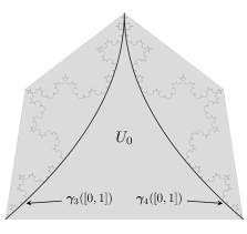
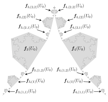
We now describe the similarity maps in . For each , the action of on the polygonal region is illustrated in Figs. 6 and 6.
To be more precise, let denote the open intervals that are removed during the construction of the middle-thirds Cantor set . Given , the interval is the middle-third interval to the left of and is the middle-third to the right, so for example,
Let and be the left and right endpoints of , respectively. Suppose that the base of has unit length, is centered at , and is aligned with the first-coordinate axis. Further suppose that its height is at most . Let , with , be parameterizations for the curves depicted in Fig. 6 with the following property: for each , and ,
We orient the curves so that corresponds to the point at the base of and is the cusp point. Put . Then
The map is the unique orientation preserving similarity transform that maps the bottom right point of to and maps the bottom left point to . On the other hand, maps to and to . With , the similarity ratio for is .
The set , considered in Example 1.1(b), is the unique compact set satisfying . Unlike finite iterated function systems, the closure is necessary [22], so is not necessarily an invariant set for . To establish the measure theoretic properties of and take advantage of its self-similarity properties, we need to identify an invariant set such that is a null set, with respect to an appropriate Hausdorff measure that will be determined later. Given and , define
If is closed and nonempty, then so is . For convenience, we will use . We point out that satisfies the open set condition: for each , we find and if . More generally, if , satisfies , for some , then . Otherwise, either or . We also observe that and
Thus, for , the set is well-defined and a singleton. In [36], it is shown that is an invariant set with respect to ; i.e.,
We can now identify . Set . Since is closed and , as , if consists of distinct indices, then and the limit points of any sequence satisfying must belong to . Since each point in is a limit point of a sequence of endpoints of the intervals removed to generate , we conclude that . By Lemma 2.1 in [36],
Since and is countable, we conclude that . We also note that is the set of so-called twist points for .
Next, we show that , and thus , has Hausdorff dimension , and argue that its -measure is finite. Since the system satisfies the open set condition, we may use a result from [22] to conclude that the Hausdorff dimension for is
In our case, the infimum is attained and is the unique solution to . The bounds for imply , where and is the unique solution to . Note, we could reduce the height of , while leaving the base unchanged, so that and . More generally, for any positive height, we find and has Hausdorff dimension . In any case, as , we conclude that, for all ,
Thus, to establish Ahlfors-regularity for , it is sufficient prove it for .
To this end, we will take advantage of some results provided by [36]. The class is clearly a conformal infinite iterated function system. The topological pressure, as defined in [36], is
Therefore, there exists a -conformal measure on . That is, has the following properties: for each ,
-
•
and ;
-
•
, for each ;
-
•
if and only if satisfy .
Lemma 4.2, in [36], implies the restriction of to , and thus , is absolutely continuous with respect to and finite. In fact, by inspecting the proof, we may deduce . In any case, as we are only interested in the -properties and -properties of , throughout the remainder of this section, we need not distinguish between and .
We now work to establish a positive lower bound for . As stated earlier, a key idea is to group subcollections of in such a way that we may work with in a manner similar to an IFS (properties (a) and (c)) below). Our objective is to show that there exists a constant such that , for all . Then, the Mass Distribution Principle [20] delivers the lower bound . Iterating the properties for stated above yields
-
•
, for all ;
-
•
if and only if , for some .
Put . Select such that . For each ,
Define ,
For convenience, given , we will use . Recall that , for . In either case, . We then may write
-
(a)
and ;
-
(b)
and ;
-
(c)
if and only if . Otherwise ;
-
(d)
.
This last property follows from and the observation that cannot exceed the diameter of the set produced by arranging the sets adjacent to each other so that their bases are adjoined along a common line, as would occur if was the Koch snowflake curve. In this case
Since each pair of sets in can only intersect in an -null set, property (b) implies
| (33) |
The scaling properties for similarly produce
| (34) |
Next, for satisfying , put
so . For each and , set
and
For any , we have and . Thus, for each and , satisfying and , there exists a , possibly equal to , such that . This implies
and thus,
| (35) |
With , we now show that , with independent of . We may assume that , so there exists and such that . By property (d), for each , we must have
and . By property (c) and the definition of , the family must consist of mutually disjoint sets. Consequently, there is an upper bound on the number of elements in . In fact, we conclude that
Using (33) and (35), we obtain
| (36) |
Since , the Mass Distribution Principle [20] implies
We have thus far shown that .
Next, we work towards establishing the Ahlfors-regulartiy for . First, with replaced by , we can incorporate (34) into the exact same argument that established (36) to prove the upper Ahlfors-regularity of . Thus, we need only show lower Ahlfors-regularity. Let and be given. For each , there exists such that and . Since , we may select such that and . By property (d), , and therefore, . By (34),
This concludes the proof.
Finally, we discuss the other claims made in Example 1.1(b). The domain is bounded by and the line segment joining the points . Let be the open subset of bounded by the curves and . For some , this wedge-shaped region is congruent to , as defined in Example 1.1(a). It is clear that satisfies hypotheses (H1) and (H2) with . Put . There is, however, no approach region for the cusp point that has both the -corkscrew and the -connectedness properties, for any and . If there were, then we could use the symmetry of and an argument similar to the one used for Lemma 2.5(d), to conclude that the set must be a -corkscrew region for , which is a contradiction. By the self-similarity of , this must also true for each point in . One easily sees that given any and , there exists . This implies fails to satisfy (H1) and (H2), for any , and thus, in particular, there is no -sided NTA neighborhood of any (see Remark 1(b)). We similarly conclude that there are no locally uniform neighborhoods of points in .
References
- [1] Achdou, Y., Sabot, C., Tchou, N.: Diffusion and propagation problems in some ramified domains with a fractal boundary. ESAIM: Mathematical Modelling and Numerical Analysis 40(4), 623–652 (2006). DOI 10.1051/m2an:2006027. URL http://www.esaim-m2an.org/10.1051/m2an:2006027
- [2] Achdou, Y., Tchou, N.: Trace theorems for a class of ramified domains with self-similar fractal boundaries. SIAM Journal on Mathematical Analysis 42(4), 1449–1482 (2010). DOI 10.1137/090747294. URL http://epubs.siam.org/doi/10.1137/090747294
- [3] Andreu-Vaillo, F., Mazón, J.M., Rossi, J.D., Toledo-Melero, J.J.: Nonlocal diffusion problems, Mathematical Surveys and Monographs, vol. 165. American Mathematical Society, Providence, RI; Real Sociedad Matemática Española, Madrid (2010). DOI 10.1090/surv/165. URL https://doi-org.libproxy.unl.edu/10.1090/surv/165
- [4] Azzam, J., Hofmann, S., Martell, J.M., Nyström, K., Toro, T.: A new characterization of chord-arc domains. J. Eur. Math. Soc. (JEMS) 19(4), 967–981 (2017). DOI 10.4171/JEMS/685. URL https://doi-org.libproxy.unl.edu/10.4171/JEMS/685
- [5] Bates, P.W., Han, J.: The Neumann boundary problem for a nonlocal Cahn–Hilliard equation. Journal of Differential Equations 212(2), 235–277 (2005). DOI 10.1016/j.jde.2004.07.003. URL https://linkinghub.elsevier.com/retrieve/pii/S0022039604002669
- [6] Brezis, H.: How to recognize constant functions. Connections with Sobolev spaces. Russian Mathematical Surveys 57(4), 693–708 (2002). DOI 10.1070/RM2002v057n04ABEH000533. URL http://stacks.iop.org/0036-0279/57/i=4/a=R02?key=crossref.0ac4b146e61752823da0889db473fb68
- [7] Capitanelli, R., Lancia, M.R., Vivaldi, M.A.: Insulating layers of fractal type. Differential and Integral Equations. An International Journal for Theory & Applications 26(9-10), 1055–1076 (2013)
- [8] Coville, J., Dupaigne, L.: On a non-local equation arising in population dynamics. Proc. Roy. Soc. Edinburgh Sect. A 137(4), 727–755 (2007). DOI 10.1017/S0308210504000721. URL https://doi-org.libproxy.unl.edu/10.1017/S0308210504000721
- [9] David, G., Feneuil, J., Mayboroda, S.: A new elliptic measure on lower dimensional sets. Acta Mathematica Sinica, English Series 35(6), 876–902 (2019). DOI 10.1007/s10114-019-9001-5. URL http://link.springer.com/10.1007/s10114-019-9001-5
- [10] David, G.R., Feneuil, J., Mayboroda, S.: Elliptic theory for sets with higher co-dimensional boundaries. arXiv preprint arXiv:1702.05503 (2017)
- [11] De Marco, G., Mariconda, C., Solimini, S.: An elementary proof of a characterization of constant functions. Advanced Nonlinear Studies 8(3), 597–602 (2008). DOI 10.1515/ans-2008-0306. URL https://doi-org.libproxy.unl.edu/10.1515/ans-2008-0306
- [12] D’Elia, M., Li, X., Seleson, P., Tian, X., Yu, Y.: A review of local-to-nonlocal coupling methods in nonlocal diffusion and nonlocal mechanics. arXiv:1912.06668 [math] (2019). URL http://arxiv.org/abs/1912.06668. ArXiv: 1912.06668
- [13] Di Biase, F.: Approach regions and maximal functions in theorems of Fatou type. ProQuest LLC, Ann Arbor, MI (1995). Thesis (Ph.D.)–Washington University in St. Louis
- [14] Diening, L., Harjulehto, P., Hästö, P., Ruzicka, M.: Lebesgue and Sobolev Spaces with Variable Exponents, Lecture Notes in Mathematics, vol. 2017. Springer Berlin Heidelberg, Berlin, Heidelberg (2011). DOI 10.1007/978-3-642-18363-8. URL http://link.springer.com/10.1007/978-3-642-18363-8
- [15] Du, Q.: Nonlocal modeling, analysis, and computation, CBMS-NSF Regional Conference Series in Applied Mathematics, vol. 94. Society for Industrial and Applied Mathematics (SIAM), Philadelphia, PA (2019). DOI 10.1137/1.9781611975628.ch1. URL https://doi-org.libproxy.unl.edu/10.1137/1.9781611975628.ch1
- [16] Du, Q., Gunzburger, M., Lehoucq, R.B., Zhou, K.: A nonlocal vector calculus, nonlocal volume-constrained problems, and nonlocal balance laws. Mathematical Models and Methods in Applied Sciences 23(03), 493–540 (2013)
- [17] Du, Q., Mengesha, T., Tian, X.: Fractional hardy-type and trace theorems for a function space of nonlocal character. preprint
- [18] Duzaar, F., Gastel, A., Mingione, G.: Elliptic systems, singular sets and Dini continuity. Comm. Partial Differential Equations 29(7-8), 1215–1240 (2004). DOI 10.1081/PDE-200033734. URL https://doi-org.libproxy.unl.edu/10.1081/PDE-200033734
- [19] Emilio Gagliardo: Caratterizzazioni delle tracce sulla frontiera relative ad alcune classi di funzioni in variabili. Rendiconti del Seminario Matematico della Università di Padova 27, 284–305 (1957)
- [20] Falconer, K.: Fractal geometry, second edn. John Wiley & Sons, Inc., Hoboken, NJ (2003). DOI 10.1002/0470013850. URL https://doi-org.libproxy.unl.edu/10.1002/0470013850. Mathematical foundations and applications
- [21] Feneuil, J., Mayboroda, S., Zhao, Z.: Dirichlet problem in domains with lower dimensional boundaries. arXiv preprint arXiv:1810.06805 p. 84 (2018)
- [22] Fernau, H.: Infinite iterated function systems. Mathematische Nachrichten 170, 79–91 (1994). DOI 10.1002/mana.19941700107. URL https://doi-org.libproxy.unl.edu/10.1002/mana.19941700107
- [23] Gal, C.G., Giorgini, A., Grasselli, M.: The nonlocal Cahn–Hilliard equation with singular potential: Well-posedness, regularity and strict separation property. Journal of Differential Equations 263(9), 5253–5297 (2017). DOI 10.1016/j.jde.2017.06.015. URL https://linkinghub.elsevier.com/retrieve/pii/S0022039617303224
- [24] Gilboa, G., Osher, S.: Nonlocal operators with applications to image processing. Multiscale Modeling & Simulation 7(3), 1005–1028 (2009). DOI 10.1137/070698592. URL http://epubs.siam.org/doi/10.1137/070698592
- [25] Giusti, E.: Precisazione delle funzioni di e singolarità delle soluzioni deboli di sistemi ellittici non lineari. Boll. Un. Mat. Ital. (4) 2, 71–76 (1969)
- [26] Hu, J.: A note on Hajłasz–Sobolev spaces on fractals. Journal of Mathematical Analysis and Applications 280(1), 91–101 (2003). DOI 10.1016/S0022-247X(03)00039-8. URL https://linkinghub.elsevier.com/retrieve/pii/S0022247X03000398
- [27] Jerison, D.S., Kenig, C.E.: Boundary behavior of harmonic functions in nontangentially accessible domains. Adv. in Math. 46(1), 80–147 (1982). DOI 10.1016/0001-8708(82)90055-X. URL https://doi-org.libproxy.unl.edu/10.1016/0001-8708(82)90055-X
- [28] Jones, P.W.: Extension theorems for BMO. Indiana University Mathematics Journal 29(1), 41–66 (1980). DOI 10.1512/iumj.1980.29.29005. URL https://doi-org.libproxy.unl.edu/10.1512/iumj.1980.29.29005
- [29] Jones, P.W.: Quasiconformal mappings and extendability of functions in sobolev spaces. Acta Mathematica 147(0), 71–88 (1981). DOI 10.1007/BF02392869. URL http://projecteuclid.org/euclid.acta/1485890130
- [30] Jonsson, A.: Besov spaces on closed subsets of . Transactions of the American Mathematical Society 341(1), 355 (1994). DOI 10.2307/2154626. URL https://www.jstor.org/stable/2154626?origin=crossref
- [31] Jonsson, A., Wallin, H.: Function spaces on subsets of . Math. Rep. 2(1), xiv+221 (1984)
- [32] Katkovnik, V., Foi, A., Egiazarian, K., Astola, J.: From local kernel to nonlocal multiple-model image denoising. International Journal of Computer Vision 86(1), 1–32 (2010). DOI 10.1007/s11263-009-0272-7. URL http://link.springer.com/10.1007/s11263-009-0272-7
- [33] Marcos, M.A.: A trace theorem for Besov functions in spaces of homogeneous type. Publicacions Matemàtiques 62, 185–211 (2018). DOI 10.5565/PUBLMAT6211810. URL http://mat.uab.cat/pubmat/articles/view_doi/10.5565/PUBLMAT6211810
- [34] Marschall, J.: The trace of Sobolev-Slobodeckij spaces on Lipschitz domains. Manuscripta Mathematica 58(1-2), 47–65 (1987). DOI 10.1007/BF01169082. URL http://link.springer.com/10.1007/BF01169082
- [35] Martio, O., Sarvas, J.: Injectivity theorems in plane and space. Annales Academiae Scientiarum Fennicae Series A I Mathematica 4, 383–401 (1979). DOI 10.5186/aasfm.1978-79.0413. URL http://www.acadsci.fi/mathematica/Vol04/vol04pp383-401.pdf
- [36] Mauldin, R.D., Urbański, M.: Dimensions and measures in infinite iterated function systems. Proceedings of the London Mathematical Society s3-73(1), 105–154 (1996). DOI 10.1112/plms/s3-73.1.105. URL http://doi.wiley.com/10.1112/plms/s3-73.1.105
- [37] Mayboroda, S., Zhao, Z.: Square function estimates, the BMO Dirichlet problem, and absolute continuity of harmonic measure on lower-dimensional sets. Analysis & PDE 12(7), 1843–1890 (2019). DOI 10.2140/apde.2019.12.1843. URL https://msp.org/apde/2019/12-7/p06.xhtml
- [38] Ros-Oton, X.: Nonlocal elliptic equations in bounded domains: a survey. Publicacions Matemàtiques 60, 3–26 (2016). DOI 10.5565/PUBLMAT˙60116˙01. URL http://mat.uab.cat/pubmat/articles/view_doi/10.5565/PUBLMAT_60116_01
- [39] Saksman, E., Soto, T.: Traces of Besov, Triebel-Lizorkin and Sobolev spaces on metric spaces. Analysis and Geometry in Metric Spaces 5(1), 98–115 (2017). DOI 10.1515/agms-2017-0006. URL http://content.sciendo.com/view/journals/agms/5/1/article-p98.xml
- [40] Shvydkoy, R., Tadmor, E.: Topological models for emergent dynamics with short-range interactions. arXiv:1806.01371 [math] (2019). URL http://arxiv.org/abs/1806.01371. ArXiv: 1806.01371
- [41] Silling, S.A.: Reformulation of elasticity theory for discontinuities and long-range forces. J. Mech. Phys. Solids p. 35 (2000)
- [42] Silling, S.A.: Peridynamics: Introduction. In: G.Z. Voyiadjis (ed.) Handbook of Nonlocal Continuum Mechanics for Materials and Structures, pp. 1–38. Springer International Publishing, Cham (2018). DOI 10.1007/978-3-319-22977-5˙29-1. URL http://link.springer.com/10.1007/978-3-319-22977-5_29-1
- [43] Tao, Y., Tian, X., Du, Q.: Nonlocal models with heterogeneous localization and their application to seamless local-nonlocal coupling. Multiscale Modeling & Simulation 17(3), 1052–1075 (2019). DOI 10.1137/18M1184576. URL https://epubs.siam.org/doi/10.1137/18M1184576
- [44] Tian, X., Du, Q.: Trace theorems for some nonlocal function spaces with heterogeneous localization. SIAM J. Math. Anal. 49(2), 1621–1644 (2017). DOI 10.1137/16M1078811. URL https://doi-org.libproxy.unl.edu/10.1137/16M1078811