TowerDebias: A Novel Debiasing Method based on the Tower Property
Abstract
Decision-making processes have increasingly come to rely on sophisticated machine learning tools, raising concerns about the fairness of their predictions with respect to any sensitive groups. The widespread use of commercial black-box machine learning models necessitates careful consideration of their legal and ethical implications on consumers. In situations where users have access to these “black-box” models, a key question emerges: how can we mitigate or eliminate the influence of sensitive attributes, such as race or gender? We propose towerDebias (tDB), a novel approach designed to reduce the influence of sensitive variables in predictions made by black-box models. Using the Tower Property from probability theory, tDB aims to improve prediction fairness during the post-processing stage in a manner amenable to the Fairness-Utility Tradeoff. This method is highly flexible, requiring no prior knowledge of the original model’s internal structure, and can be extended to a range of different applications. We provide a formal improvement theorem for tDB and demonstrate its effectiveness in both regression and classification tasks, underscoring its impact on the fairness-utility tradeoff.
Keywords: Algorithmic Fairness, Tower Property of Conditional Expectation, Fairness-Utility Tradeoff, Post-Processing Mitigation Techniques, AI Ethics in Decision-Making
1 Introduction
In recent years, the rapid development of machine learning algorithms and their extensive commercial applications have become increasingly relevant across domains like cybersecurity, healthcare, e-commerce, and more (Sarker, 2021). As these models increasingly guide critical decision-making processes with real-world consequences for consumers, a noteworthy concern has emerged: algorithmic fairness in machine learning (Wehner and Köchling, 2020; Chen, 2023). The primary objective of ensuring fairness in machine learning is to reduce the impact of sensitive attributes—such as race, gender, and age—on an algorithm’s predictions.
A seminal case in the field of fair machine learning is the development of the COMPAS (Correctional Offender Management Profiling for Alternative Sanctions) algorithm by Northpointe, designed to assess a criminal’s likelihood of recidivism. The goal of this tool is to assist judges in making sentencing decisions.
However, COMPAS came under intense scrutiny after an investigation by ProPublica, which revealed evidence of racial bias against black defendants compared to white defendants with similar profiles (Angwin et al., 2016). Northpointe contested these findings, asserting that their software treated Black and White defendants equally. In response, ProPublica issued a detailed rejoinder, making its statistical methods and findings publicly available (Angwin and Larson, 2016). While we do not take a position on the specific dispute, this case highlights the critical importance of addressing fairness in machine learning.
A key issue with “black box” algorithms like COMPAS is that the purchaser cannot easily remove the sensitive variables (), such as race, and rerun the algorithm. The source code of the algorithm is typically not accessible, and the training data is often unavailable as well. This raises a crucial question: how can we reduce or eliminate the influence of in such cases? This paper aims to address this challenge.
1.1 The Setting
We consider prediction of a variable from a feature vector X and a vector of sensitive variables . The target may be either numeric (in a regression setting) or dichotomous (in a two-class classification setting where = 1 or = 0). The -class case can be handled using dichotomous variables with regards to the material presented here.
Consider an algorithm developed by a vendor, such as COMPAS, which was trained on data . This data can be assumed to originate from some specific data-generating process, with the algorithm’s initial objective being to estimate . However, the client who purchased the algorithm wishes to exclude and instead estimate 111Quantities of the form E(), P(), Var() and so on refer to the probability distribution of the data generating process..
In the regression setting, we assume squared prediction error loss to minimize error. In the classification setting, we define:
where the predicted class label is given by:
This approach minimizes overall misclassification rate by selecting the class with the highest predicted probability.
Several potential use cases for employing tDB can be identified:
-
(a)
The client has no knowledge of the internal structure of the black-box algorithm and lacks access to the original training data. Thus, the client will need to gather their own data from new cases that arise during the tool’s initial use.
-
(b)
Client has no knowledge of the inner workings of the black-box algorithm but is given the training data.
-
(c)
User of the algorithm, potentially even the original developer, knows the black-box’s details and possesses the training data. He/she is satisfied with the performance of the algorithm, but desires a quick, simple way to remove the influence of in its predictions.
In each setting, the individual aims to predict new cases using only . The client either does not know or chooses to disregard it. In other words, although the algorithm provides estimates of , the goal is to use instead as the prediction instead. In other words, even though the algorithm gives us an estimated , we wish to instead use estimated as our prediction. In this paper, we present tDB as an innovative approach to modify the predictions of the original algorithm, bypassing the “black box” nature of the model.
1.2 Introducing the Fairness-Utility Tradeoff
Many commercial black-box models may include sensitive variables, which raises significant ethical and legal concerns. In the pursuit of fairness, a fundamental Fairness-Utility tradeoff emerges: a delicate balance between fairness and predictive accuracy (Gu et al., 2022; Sun et al., 2023). This tradeoff highlights that prioritizing fairness often leads to a reduction in accuracy. However, the extent of this tradeoff is influenced by the specific fairness metrics employed and their implementation details. This paper explores the impact of applying tDB on the fairness-utility tradeoff across different datasets, encompassing both regression and classification tasks.
1.3 Paper Outline
The paper is organized as follows: Section 2 reviews prior literature on fair machine learning, focusing on relevant methods and proposed fairness metrics; Section 3 introduces the towerDebias algorithm and provides supporting proofs demonstrating fairness improvements; Section 4 presents empirical results of tDB on multiple datasets; and Section 5 concludes with a discussion and future directions.
2 Related Work
A significant body of literature has been published in the field of algorithmic fairness, focusing on addressing critical social issues related to mitigating historical bias in data-driven applications. For example, Chouldechova (2017) examines the use of Recidivism Prediction Instruments in legal systems, highlighting the potential disparate impact on racial groups. Collaborative efforts from the Human Rights Data Analysis Group and Stanford University have developed additional frameworks for fair modeling (Lum and Johndrow, 2016; Johndrow and Lum, 2019). In particular, significant research has focused on fair binary classification, see: Barocas et al. (2023); Zafar et al. (2019). More recently, Denis et al. (2024) extends these concepts to multi-class classification from a fairness perspective.
Broadly speaking, fairness criteria can generally be categorized into two measures: group fairness and individual fairness. The central idea behind individual fairness is that similar individuals should be treated similarly (Dwork et al., 2012), though the specific implementation details may vary. One approach to individual fairness is propensity score matching (Karimi et al., 2022). In contrast, group fairness requires predictions to be similar across different groups as defined by the sensitive attributes. Commonly used measures of group fairness include demographic parity and equality of opportunity (Hardt et al., 2016).
Much work has been proposed to integrate fairness constraints at various stages of the machine learning deployment pipeline (Kozodoi et al., 2022). Pre-processing involves removing bias from the original dataset before training the model, with several proposed methods outlined in Calmon et al. (2017); Zemel et al. (2013); Wiśniewski and Biecek (2021); Madras et al. (2018). In-processing refers to incorporating fairness constraints during the model training process (Komiyama et al., 2018; Scutari, 2023; Agarwal et al., 2019). Post-processing involves adjusting predictions after the model has been trained (Hardt et al., 2016; Silvia et al., 2020). Notably, a considerable amount of research has focused on achieving fairness through ridge penalties in linear models (Scutari, 2023; Komiyama et al., 2018; Zafar et al., 2019; Matloff and Zhang, 2022). tDB employs a post-processing approach, as we are modifying the predictions of the original black-box models to achieve fairness.
2.1 Measuring Fairness
Already, much literature has been published on different fairness measures, many of which are complex and require substantial domain-specific knowledge. In this section, we discuss some widely accepted fairness measures:
-
(a)
Demographic Parity: This fairness criterion evaluates group fairness by requiring that individuals from both marginalized and non-marginalized groups have an equal probability of being assigned to the positive class, regardless of group membership. For a binary and , it can be expressed as:
In this equation, the probability of being assigned to the positive class (1) is the same for both Group = 0 and Group = 1, indicating group fairness. Thus, demographic parity requires that the prediction be independent of the protected attribute, meaning that membership to a protected class should not be correlated with the outcome variable.
-
(b)
Equalized Odds: This criterion offers a more robust measure of group fairness compared to demographic parity. It requires that the predictor satisfies equalized odds with respect to the protected attribute and the outcome , if and are independent conditional on . For binary and , this can be expressed as:
For the outcome , this constraint requires that has equal true positive rates across the two demographics, and . For , the constraint ensures equal false positive rates. In this way, equalized odds requires that the model maintains consistent accuracy across all demographic groups, penalizing models that perform well only on the majority group (Hardt et al., 2016).
-
(c)
Correlation : Correlation-based measures are commonly used in fairness evaluation (Deho et al., 2022; Mary et al., 2019). Baharlouei et al. (2019) extends fairness measurement to continuous variables by applying the Renyi maximum correlation coefficient. Lee et al. (2022) introduces a maximal correlation framework for formulating fairness constraints. Roh et al. (2023) explores the concept of correlation shifts in the context of fair training. In general, correlations between predicted and can be expressed as:
In this paper, we apply correlation-based measures to evaluate fairness between our predicted and the sensitive attribute . Specifically, we use the Kendall’s Tau correlation coefficient to examine the relationships between these variables. Kendall’s Tau is a non-parametric measure that captures both the strength and direction of the association, making it well-suited for data on an ordinal or categorical scale. We choose Kendall’s Tau over other correlation measures, such as Pearson’s correlation, because it does not require the assumption of linearity, allowing us to assess relationships even when or are categorical or binary (KENDALL, 1938).
For categorical , we apply one-hot encoding to create dummy variables for each category, then compute Kendall’s Tau for each category separately to assess the individual reduction in correlation. Lower values (closer to 0) of Kendall’s Tau indicate reduced association between the predictions from the black-box model and , which reflects higher fairness. Since interpreting the direction of association is not the primary focus of our fairness analysis, we use the absolute value of Kendall’s Tau to evaluate the overall reduction in correlation between predictions and .
2.2 Measuring Accuracy
Assessing accuracy is generally more straightforward than evaluating fairness. In regression tasks, we measure accuracy using the Mean Absolute Prediction Error (MAPE), which calculates the average absolute difference between the predicted and true values. For binary classification tasks, we measure accuracy using the overall misclassification rate to represent the proportion of incorrect predictions among all predictions made.
3 Introducing TowerDebias
The heart of this algorithm is based on a well-known theorem from measure-theoretic probability. In this section, we present the theorem, explain its intuitive meaning, and then demonstrate its application to our algorithm.
3.1 Tower Property of Conditional Expectation
The Tower Property of conditional expectation (Wolpert, 2009) states:
| (3.1) |
The Tower Property of conditional expectation expresses that the conditional expectation of given can be decomposed into the conditional expectation of given both and a sensitive attribute , then conditioned again on . Note that conditional expectations themselves are random variables. For example, —as a function of the random variable —is itself a random variable.
To illustrate this property intuitively, consider the following example using a dataset that will be referenced later in the paper. This dataset includes: , a score on the Law School Admissions Test; , family income (five quintile levels); and , race. What does equation (3.1) mean at the “population” level of the data generating process?
For instance, is the mean LSAT score for Black test-takers in the fourth income quintile. Now, consider the expression:
This quantity averages the mean LSAT score for income level 4 over all races. (3.1) then states that this average will equal the overall mean score for income level 4, regardless of race. This aligns with our intuition: conditioning on income (level 4) and then averaging over all races gives the same result as directly conditioning on income alone. Note that the averaging is weighted by the probabilities of the various races.
3.2 Relation to towerDebias
In simple terms, our method can be summarized as follows:
To remove the impact of the sensitive variable on predictions of from , average the predictions over .
(3.1) is, of course, an idealization at the population or data-generating process level. However, in practical situations, the vendor’s black-box algorithm can only estimate from training data, , . In such cases, what additional factors must be considered?
Let’s revisit the LSAT example, now adding the features undergraduate GPA and cluster (an indicator of the law school’s ranking). Now , and suppose we want to predict a new case where . Using tDB, we would take the average LSAT scores for all cases in our training data that match this exact value of . However, it turns out that there are only 7 such cases in our dataset—hardly enough to obtain a reliable average. Furthermore, if income were measured in dollars rather than quintiles, or if GPA were available to two decimal places, there might be no cases at all matching this exact value.
The solution is to instead average over all cases near the given value of . To do this, we introduce a new parameter, , which represents the number of training cases whose values will be averaged—specifically, the cases nearest to the value we want to predict.222This parameter is analogous to in the K-Nearest Neighbors method.
Choosing the right is crucial to balancing the influence of the sensitive variable. In particular, defines the number of neighboring rows used to compute the average LSAT score. A small might lead to an overly narrow selection of cases, resulting in minimal reduction in correlation with the sensitive variable. Conversely, a larger may include rows that are too distant and not representative of the new data point being debiased. Thus, choosing an appropriate is extremely important as it must balance the need for a sufficiently large sample size while maintaining proximity to the target data point. As we will see in the empirical section, this choice of has a considerable impact on the fairness-utility tradeoff.
The next two parts of this section present supporting proofs for the reduction in correlation when applying tDB. Section 3.3 provides an expression for Pearson correlation reduction in a simulated trivariate normal case. Section 3.4 extends this concept to more general cases, using vector spaces to indicate fairness improvements.
3.3 Measuring Correlation Reduction—Trivariate Normal Case
Suppose we are predicting using a single numeric feature and a numeric . We assume that (X,S,Y) follows a trivariate normal distribution. This implies that the joint distribution of is normal, and therefore, each individual variable , , and also has a marginal normal distribution (Johnson and Wichern, 1993).
Our goal is to derive a closed-form expression for the reduction in Pearson correlation between the predicted and when predicting from both (Case I) versus predicting from just (Case II). In this simulation, we are specifically interested in assessing the reduction in the Pearson correlation, as opposed to using Kendall’s Tau correlation used in the tDB method.
The choice of Pearson correlation in this context is motivated by the nature of the trivariate normal distribution. The Pearson correlation coefficient quantifies the strength of the linear relationship between two numeric variables (Faizi and Alvi, 2023). Its inherent linearity properties across both the numerator and denominator of its formula helps facilitate simplification for our expressions. Specifically, the numerator of Pearson’s correlation involves computing and exhibits bilinearity in the random variables and . This bilinearity property allows us to simplify expressions by factoring out any constants and leveraging additivity.
In contrast, Kendall’s Tau lacks such linearity properties, which makes it less conducive to similar simplifications. Thus, Pearson correlation is better suited for this particular example, as it enables the derivation and analysis of a closed-form expression for the reduction in correlation between the two cases. This choice provides a clear and interpretable framework for examining the impact of predicting from both and versus predicting solely from .
Given our application, the general formula for calculating the Pearson correlation coefficient333This general will be used to compute the correlations in both Case I and Case II. between the predicted and is as follows (Mukaka, 2012):
To proceed, let’s first define key quantities using regression coefficients to represent the relationships among , , and . These will be important in calculating correlation reductions between Case I and Case II.
In Case I, where we predict using , the linear relationship of the predicted —denoted as —can be represented as follows:
Here:
-
•
is the intercept term,
-
•
is the coefficient for ,
-
•
is the coefficient for .
For Case II, we may express the linear relationship to predict solely from —denoted as —as follows:
Similarly, we define:
-
•
is the intercept term,
-
•
is the coefficient for .
Note that since each case uses a different set of predictors to estimate , the resulting predictions— and —will be different. We are interested in finding a closed-form expression for the difference in correlations between Case I and Case II for , which can be defined as:
Furthermore, given the assumption of a trivariate normal distribution, the linear relationship between and allows us to model as a function of . Note that we are focusing on modeling , instead of , as in the previous examples for . The inclusion of the term accounts for any errors. Thus, this relationship can be expressed as:
In this model:
-
•
is the intercept term,
-
•
is the coefficient for ,
-
•
is the error term, normally distributed with mean zero and variance , and is independent of the predictor terms and (Kutner et al., 1974).
Now that we have defined the necessary quantities to model the relationship between the given variables, we can proceed with finding .
Case I: Compute
To begin, we may define as:
Step 1: Simplifying the Covariance
By the bilinearity property of covariance, we can expand the numerator as follows:
Since is a constant, . Moreover, and , where is the variance of .
Thus, we have:
We can further simplify the expression for using the variable relationship quantities that we have derived.
Step 2: Computing
Next, we compute .
Since is a constant, , and since is independent of , . Therefore, we are left with:
where is the variance of .
Step 3: Final Expression for
Substituting the result for into the expression for yields
Finally, we can express the correlation as:
This is our simplified expression for the correlation between and .
Case II: Compute
Similarly, we may define as:
Step 1: Simplifying the Covariance
Using a similar process as shown in Case I, we can simplify :
Step 2: Final Expression for
Then, can be written as:
This is our simplified expression for the correlation between and .
Final Step: Compute
Thus, is:
| (3.3) |
This expression quantifies the reduction in Pearson correlation between and between Case I (with both and as predictors) and Case II (with only ).
3.4 Measuring Correlation Reduction—Generalized Case
Fairness improvements can be established more broadly, extending beyond the simulated trivariate normal case, through the use of function spaces. This section will demonstrate the proof for this scenario.444More details to be added.
4 Empirical Study
Our empirical analysis demonstrates the effectiveness of tDB on the fairness-utility tradeoff across several well-known datasets in fair machine learning, encompassing both regression and classification tasks. The analysis includes five datasets: SVCensus, Law School Admissions, COMPAS, Iranian Churn, and Dutch Census.
To establish baseline results for fairness and accuracy, we train several machine learning models to generate the initial predictions. tDB is then applied to each model’s individual predictions to evaluate the improvement in fairness—measured as a reduction in —at some potential cost in predictive performance. Our study aims to explore how varying choices of the tradeoff parameter , selected based on the specific algorithm and dataset, impacts the overall applicability of this method and the balance over the fairness-utility tradeoff.
We train several conventional machine learning models, including Linear & Logistic Regression, K-Nearest Neighbors, XGBoost, and Deep Neural Networks to establish baseline results. The Quick And Easy Machine Learning (qeML) package in R provides a user-friendly framework for constructing models and generating predictions for Linear & Logistic Regression, K-Nearest Neighbors, and XGBoost. The Neural Network was trained using the PyTorch package in Python.
We also set fair baseline predictions from the fairML package using functions defined in Scutari (2023), Komiyama et al. (2018), and Zafar et al. (2019). These algorithms include Fair (Generalized) Ridge Regression, and Zafar’s Linear & Logistic Regression models. Note that the fairML functions already incorporate fairness constraints into their predictions, and we set the unfairness parameter to 0.1. By setting the unfairness parameter to this value, fairness is prioritized within the training process itself, and we aim to achieve further improvements with tDB. Additional details on the training processes for baseline models can be found on GitHub555TowerDebias Github repository: https://github.com/matloff/towerDebias..
Results from our analysis are presented graphically, highlighting comparative outcomes in MAPE/misclassification rate increase and correlation reductions. Note: The graphs illustrate the relative changes in fairness and accuracy compared to the baseline models. For instance, if K-Nearest Neighbors initially has a misclassification rate of 0.2, a 10% increase with the application of tDB implies the new misclassification rate rises to 0.22. The same idea applies for correlation reductions. Our objective is to highlight the comparative gains in fairness (and the corresponding trade-off in accuracy) achieved over existing methods.666To reduce sampling variability, we use 25 holdout sets and calculate the average test accuracy and correlation coefficient.
| Dataset | Response Variable Y | Sensitive Variable(s) S | Rows/# of Predictors |
|---|---|---|---|
| SVCensus | Wage Income (Continuous) | Gender (Male/Female) | 20,090/5 |
| Law School Admissions | LSAT Score (Continuous) | Race (White, Black, Hispanic, Asian, Other) | 20,800/10 |
| COMPAS | Recidivism (Binary: Yes/No) | Race (White, Black, Hispanic) | 5,497/14 |
| Iranian Churn | Exit Status (Binary: Yes/No) | Gender (Male/Female), Age (Continuous) | 10,000/10 |
| Dutch Census | Occupation (Binary: high status/low status) | Gender (Male/Female) | 60,420/11 |
A key question from our experiments is the selection of an appropriate value for . We aim to avoid values that are too small or too large. The experiments offer insights into the fairness-utility tradeoff, helping guide the optimal choice of in applying tDB.
4.1 SVCensus
The SVCensus dataset is a subset of U.S. Census data from the early 2000s, focusing on income levels across six engineering occupations within Silicon Valley. Each person’s record in the dataset includes attributes such as occupation, education level, number of weeks worked, and age. Our goal is to predict wage income () with respect to gender as the sensitive attribute (). Note that this is regression problem, and gender contains two categories: male and female.


The graphs above illustrate the fairness-accuracy tradeoffs from applying towerDebias method to the baseline model predictions. Figure (1) shows the improvement in fairness—the reduction in correlation between predicted wage income and gender—and Figure (2) displays the comparative losses in accuracy.
The tDB method demonstrates substantial reductions in correlations across different values of the tradeoff parameter . When applied to the predictions of traditional machine learning algorithms, tDB achieves a notable reduction in correlations, with decreases of up to 50% compared to baseline results. For instance, the initial correlations for Linear Regression, K-NN, and Neural Networks were around 0.25, while tDB reduced these correlations to below 0.1, even at smaller values of . In contrast, the fairML methods had already incorporated fairness in their baseline predictions to achieve smaller initial correlations, but tDB still provided further improvements. However, in Zafar’s Linear Regression model, which started with a relatively low initial correlation of 0.1, tDB did not display any further reductions.
Regarding accuracy, tDB shows modest losses in comparative MAPE results for both traditional and fair machine learning algorithms. For traditional models, the baseline accuracy averaged around $25,000, with only a slight decrease in accuracy after applying tDB. Even at higher values of (k 30), the relative loss in accuracy was less than 5% as compared to the original results. In fact, for XGBoost, the error appears decrease by $2,000—indicating a simultaneous improvement in both fairness and accuracy measures. For the fairML algorithms, which initially had a higher MAPE of approximately $35,000, the impact of tDB was even less significant, resulting in less than a 1% reduction in accuracy.
Both Figures (1) and (2) highlight the effect on the fairness-utility tradeoff on the SVCensus data. Overall, applying tDB on this dataset across various baseline model predictions results in considerable correlation reductions between predicted income and gender, , to highlight improvements in fairness with minimal loss in predictive accuracy. This underscores the effectiveness of tDB in controlling the influence of the sensitive variable and producing fairer predictions.
4.2 Law School Admissions
The Law School Admissions dataset777Note that the data pertains to students who were already admitted to law school, so despite the title, it does not relate to the admissions process itself. is a survey of law school students in the United States from 1991. It includes various demographic and academic details, such as age, grade decile score, undergraduate GPA, family income, gender, race, and more. The dataset is used to predict LSAT scores (), with race considered as the sensitive attribute (). This is a regression task, where race is categorized into the following groups: Asian, Black, White, Other, and Hispanic. This setup broadens the scope of fairness measurement beyond binary sensitive attributes, such as gender, as shown in the previous example with the SVCensus data.


Similar to the results in the SVCensus data, Figure (3) demonstrates improvements in fairness—reduction in the correlation between predicted LSAT scores and each individual racial category—and Figure (4) presents the relative increase in MAPE in comparison to the baseline predictions.
In terms of fairness, we present individual results for each racial category: White, Black, Hispanic, Asian, and Other. Figure (3) illustrates the effectiveness of applying towerDebias across various baseline algorithms to produce considerable reduction in correlations between different racial groups. Notably, each racial group exhibited different baseline correlations. For instance, in the neural network baseline model, the correlation between predicted LSAT scores and “African American” and “White” was 0.3, while for “Asian” and “Other” it was below 0.1, and for “Hispanic”, it was 0.15. Similar correlations results were observed in the other traditional machine learning model predictions. Concerning the fairML functions, the baseline results showed smaller initial correlations due to the fairness constraints integrated into the model, but there was still some slight variation between the racial groups. In applying to towerDebias, we see an decrease of more than 50% across all of the racial groups starting at moderate values of the trade-off parameter .
The accuracy results are similar to those observed in the SVCensus data. For example, the initial algorithms have a mean absolute prediction error of approximately 3.5, and applying towerDebias leads to an accuracy loss of less than 5% across different values of . Interestingly, when towerDebias is applied to XGBoost, it actually improves accuracy, suggesting enhancements in both fairness and accuracy—warranting further investigation. The selection of rows showed a slight decrease in error, indicating potential improvements in predictive power. The fair machine learning algorithms initially performed similarly to conventional algorithms. Notably, the application of towerDebias resulted in a controlled increase in accuracy, with Zafar’s model experiencing a slight decrease and the Scutari method showing less than a 1% improvement.
Both the Law School Admissions and SVCensus datasets underscore the effectiveness of applying tDB to the fairness-utility tradeoff in regression settings. Our results consistently demonstrate this method effectiveness in reducing the influence of sensitive variables across multiple models and sensitive groups. This highlights the capability of tDB on improve fairness with only a modest reduction in utility. The next phase of experiments will focus on extending this method to classification scenarios.
4.3 COMPAS
The COMPAS dataset, which contains data on criminal offenders screened in Florida during 2013-14, is being used to predict the likelihood that a defendant will recommit a crime in the near future (probability of recidivism—denoted as ). Race is treated as the sensitive variable (), with the data pre-processed to include three racial categories: White, African American, and Hispanic. The task is now a binary classification problem where race is considered a categorical variable with three possible values.
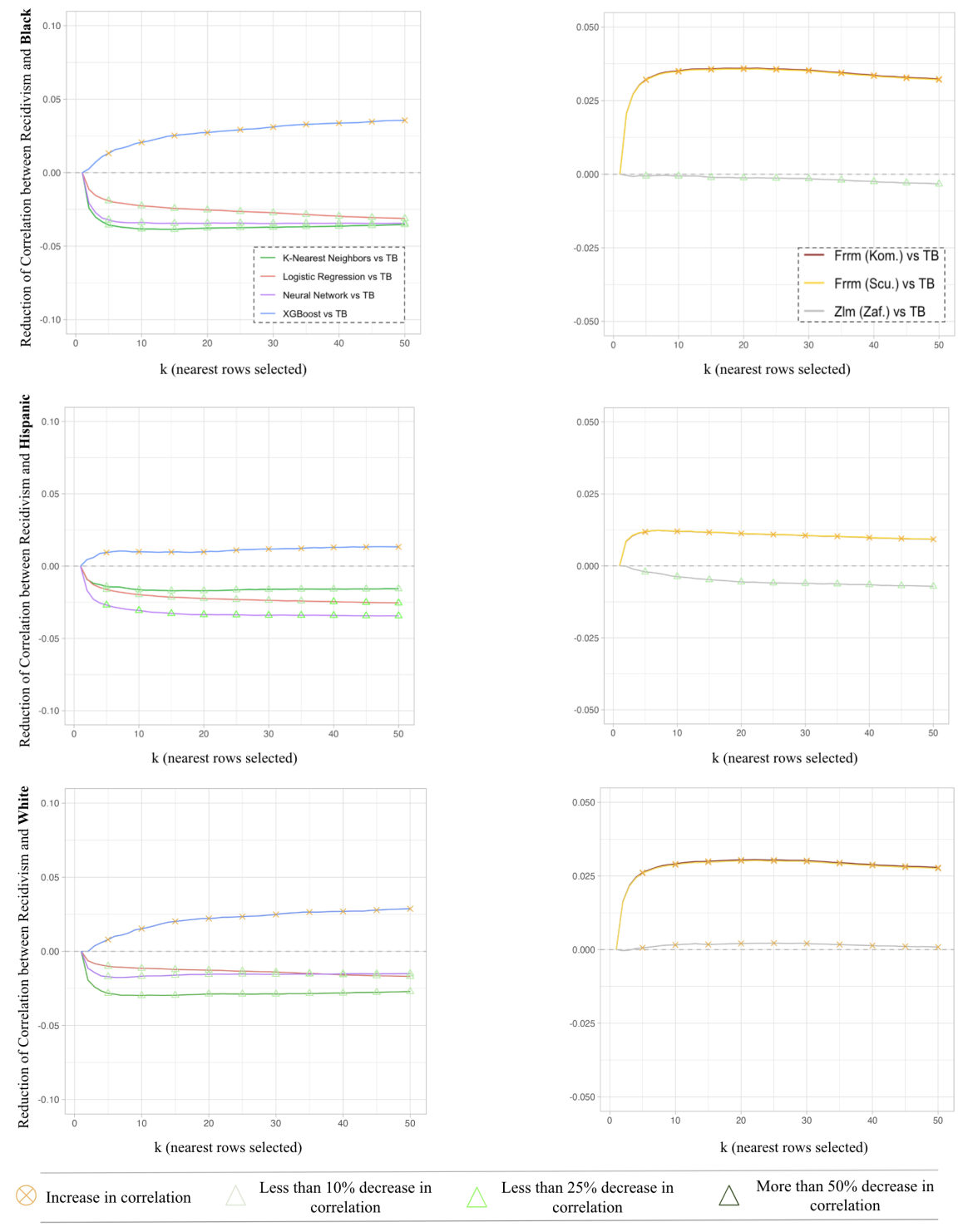

An analysis of tDB’s impact on individual algorithms in the COMPAS dataset reveals nuanced outcomes. Logistic Regression, K-Nearest Neighbors, and Neural Networks showed similar fairness improvements, with tDB consistently reducing correlations between predictions () and sensitive attributes () across racial groups. Although baseline correlations varied by race, they consistently decreased with tDB; for example, as increased, for African Americans dropped from 0.23 to 0.2, with comparable reductions for Caucasians and Hispanics. KNN and Neural Networks echoed these fairness gains, though with some tradeoff in utility. In contrast, tDB applied to XGBoost showed an unexpected increase in for each race as increased, suggesting a need for further investigation.
Analysis of tDB’s fairness outcomes across fairML functions is similar. Ridge Regression models and Zafar’s Logistic Regression initially had lower correlations with sensitive attributes than traditional models, and tDB further enhanced fairness. In contrast, Scutari and Komiyama methods, like XGBoost, showed increased correlations with tDB, while Zafar’s Logistic Regression reduced correlation further for Hispanic and African American groups, maintaining a stable misclassification rate without increase.
In terms of accuracy, we observe a slight increase in misclassification rates. For example, Logistic Regression’s initial misclassification rate of 0.27 saw less than a 10% increase as tDB was applied to more rows. Overall, the utility loss remains controlled—with notable fairness gains—underscoring tDB’s effectiveness in improving fairness within the COMPAS dataset in classification settings.
4.4 Iranian Churn
The Iranian Churn dataset is used to predict customer churn, with “Exited” as the response variable and “Gender” and “Age” as the sensitive variables. In this example, we incorporate a continuous sensitive variable to extend the analysis beyond categorical or binary .


Figure (7) illustrates the impact on correlation for Gender and Age, demonstrating the effectiveness of tDB in reducing correlations for continuous sensitive variables. Similar trends are observed, with correlations decreasing by more than 50% compared to the initial baseline results in both categories. The results from the fairML functions showed mixed trends: applying tDB reduced correlation with respect to Age but increased it for Gender.
In terms of accuracy, Figure (8) shows a modest increase in the misclassification rate for conventional machine learning algorithms compared to tDB. Logistic Regression and K-Nearest Neighbors exhibit relative increases of less than 10% and 25%, respectively, while XGBoost and Neural Networks show increases exceeding 25% for mid-to-high values. Notably, accuracy remains unchanged when comparing fairML with tDB.
4.5 Dutch Census
The Dutch Census dataset, collected by the Dutch Central Bureau for Statistics in 2001, is used to predict whether an individual holds a prestigious occupation or not (binary response variable), with “gender” as the sensitive attribute. Note: Zafar’s Logistic Regression encountered errors in training and was excluded from our analysis. The following graphs illustrate the impact of tDB across several models.
Empirical results from the Dutch Census dataset demonstrate significant improvements in fairness with a controlled accuracy loss on classification tasks. The dataset includes 10 categorical predictors, and tDB applies one-hot encoding to convert these into dummy variables, increasing the dimensionality to 61 predictors. This example highlights tDB’s effectiveness on high-dimensional, sparse datasets. Thus, this examples illustrates the effectiveness of tDB on high-dimensional, sparse datasets. In terms of fairness, Figure (9) shows considerable reductions in correlations when applying tDB to both traditional and fair machine learning models. For mid-to-high range of values, the correlation reduction exceeds 50% compared to the baseline results. Regarding accuracy, Figure (10) hows that tDB leads to a 25% increase in the misclassification rate at mid-to-high range values for traditional machine learning models, with similar trends observed in comparisons between fairML functions and tDB.
Insights from the COMPAS, Iranian Churn, and Dutch Census datasets highlight the impact of tDB on the fairness-utility tradeoff in classification settings. The consistent reduction in correlation between sensitive variables and predictions across different models underscores the effectiveness of tDB in enhancing fairness, albeit with some utility tradeoff. Overall, these findings suggest that our method shows strong potential for improving fairness in both regression and classification scenarios.
Choosing an appropriate
As observed in the tDB plots, selecting an appropriate value for significantly impacts the fairness-utility tradeoff. General trends show a notable decrease in correlation at lower values, with the reductions stabilizing once reaches around 10. Thus, one could identify the “elbow” point, analogous to the choice of clusters in k-means clustering, as additional fairness improvements become marginal. This approach helps control accuracy losses, as selecting smaller values of minimizes the impact on utility.


5 Discussion
Empirical evaluations of the towerDebias (tDB) method across conventional machine learning algorithms yield promising results. This approach achieves a significant reduction in with only a modest utility loss. While results varied across datasets and methods, most cases showed a clear decrease in the correlation coefficient. The study highlights the importance of selecting appropriate values in the tDB approach, as this choice plays a key role in minimizing the impact of sensitive variables while balancing utility. Findings suggest that the optimal depends on the specific dataset and algorithm.
In summary, the empirical evidence supports tDB as an effective tool for improving fairness in machine learning. This study contributes to ongoing fair machine learning research and provides a basis for further exploration and refinement of methods to address algorithmic bias.
References
- Agarwal et al. [2019] Alekh Agarwal, Miroslav Dudík, and Zhiwei Steven Wu. Fair regression: Quantitative definitions and reduction-based algorithms. In International Conference on Machine Learning, pages 120–129. PMLR, 2019.
- Angwin and Larson [2016] Julia Angwin and Jeff Larson. Machine bias: Technical response to northpointe, 2016. URL https://www.propublica.org/article/technical-response-to-northpointe.
- Angwin et al. [2016] Julia Angwin, Jeff Larson, Surya Mattu, and Lauren Kirchner. Machine bias, 2016. URL https://www.propublica.org/article/machine-bias-risk-assessments-in-criminal-sentencing.
- Baharlouei et al. [2019] Sina Baharlouei, Maher Nouiehed, Ahmad Beirami, and Meisam Razaviyayn. R’enyi fair inference. arXiv preprint arXiv:1906.12005, 2019.
- Barocas et al. [2023] Solon Barocas, Moritz Hardt, and Arvind Narayanan. Fairness and Machine Learning: Limitations and Opportunities. MIT Press, 2023.
- Calmon et al. [2017] Flavio Calmon, Dennis Wei, Bhanukiran Vinzamuri, Karthikeyan Natesan Ramamurthy, and Kush R Varshney. Optimized pre-processing for discrimination prevention. Advances in neural information processing systems, 30, 2017.
- Chen [2023] Zhisheng Chen. Ethics and discrimination in artificial intelligence-enabled recruitment practices. Humanities and Social Sciences Communications, 10, 09 2023. doi: 10.1057/s41599-023-02079-x.
- Chouldechova [2017] Alexandra Chouldechova. Fair prediction with disparate impact: A study of bias in recidivism prediction instruments. Big data, 5(2):153–163, 2017.
- Deho et al. [2022] Oscar Deho, Chen Zhan, Jiuyong Li, Jixue Liu, Lin Liu, and Thuc le. How do the existing fairness metrics and unfairness mitigation algorithms contribute to ethical learning analytics? British Journal of Educational Technology, 53:1–22, 04 2022. doi: 10.1111/bjet.13217.
- Denis et al. [2024] Christophe Denis, Romuald Elie, Mohamed Hebiri, and François Hu. Fairness guarantees in multi-class classification with demographic parity. Journal of Machine Learning Research, 25(130):1–46, 2024. URL http://jmlr.org/papers/v25/23-0322.html.
- Dwork et al. [2012] Cynthia Dwork, Moritz Hardt, Toniann Pitassi, Omer Reingold, and Richard Zemel. Fairness through awareness. In Proceedings of the 3rd innovations in theoretical computer science conference, pages 214–226, 2012.
- Faizi and Alvi [2023] Nafis Faizi and Yasir Alvi. Correlation. In Biostatistics Manual for Health Research, pages 109–126. ScienceDirect, 2023.
- Gu et al. [2022] Xiuting Gu, Zhu Tianqing, Jie Li, Tao Zhang, Wei Ren, and Kim-Kwang Choo. Privacy, accuracy, and model fairness trade-offs in federated learning. Computers & Security, 122:102907, 09 2022. doi: 10.1016/j.cose.2022.102907.
- Hardt et al. [2016] Moritz Hardt, Eric Price, and Nati Srebro. Equality of opportunity in supervised learning. Advances in neural information processing systems, 2016. URL https://arxiv.org/abs/1610.02413.
- Johndrow and Lum [2019] James E Johndrow and Kristian Lum. An algorithm for removing sensitive information. The Annals of Applied Statistics, 13(1):189–220, 2019.
- Johnson and Wichern [1993] Richard Johnson and Dean Wichern. Applied Multivariate Statistical Analysis. Pearson, 1993.
- Karimi et al. [2022] Hamid Karimi, Muhammad Fawad Akbar Khan, Haochen Liu, Tyler Derr, and Hui Liu. Enhancing individual fairness through propensity score matching. In 2022 IEEE 9th International Conference on Data Science and Advanced Analytics (DSAA), pages 1–10, 2022. doi: 10.1109/DSAA54385.2022.10032333.
- KENDALL [1938] M. G. KENDALL. A NEW MEASURE OF RANK CORRELATION. Biometrika, 30(1-2):81–93, 06 1938. ISSN 0006-3444. doi: 10.1093/biomet/30.1-2.81. URL https://doi.org/10.1093/biomet/30.1-2.81.
- Komiyama et al. [2018] Junpei Komiyama, Akiko Takeda, Junya Honda, and Hajime Shimao. Nonconvex optimization for regression with fairness constraints. In Jennifer Dy and Andreas Krause, editors, Proceedings of the 35th International Conference on Machine Learning, volume 80 of Proceedings of Machine Learning Research, pages 2737–2746. PMLR, 10–15 Jul 2018. URL https://proceedings.mlr.press/v80/komiyama18a.html.
- Kozodoi et al. [2022] Nikita Kozodoi, Johannes Jacob, and Stefan Lessmann. Fairness in credit scoring: Assessment, implementation and profit implications. European Journal of Operational Research, 2022.
- Kutner et al. [1974] Michael Kutner, Christopher Nachtsheim, John Neter, and William Li. Applied Linear Statistical Models. 1974.
- Lee et al. [2022] Joshua Lee, Yuheng Bu, Prasanna Sattigeri, Rameswar Panda, Gregory Wornell, Leonid Karlinsky, and Rogerio Feris. A maximal correlation approach to imposing fairness in machine learning. In ICASSP 2022-2022 IEEE International Conference on Acoustics, Speech and Signal Processing (ICASSP), pages 3523–3527. IEEE, 2022.
- Lum and Johndrow [2016] Kristian Lum and James Johndrow. A statistical framework for fair predictive algorithms. arXiv preprint arXiv:1610.08077, 2016.
- Madras et al. [2018] David Madras, Elliot Creager, Toniann Pitassi, and Richard Zemel. Learning adversarially fair and transferable representations. In International Conference on Machine Learning, pages 3384–3393. PMLR, 2018.
- Mary et al. [2019] Jérémie Mary, Clément Calauzènes, and Noureddine El Karoui. Fairness-aware learning for continuous attributes and treatments. In International Conference on Machine Learning, 2019. URL https://api.semanticscholar.org/CorpusID:174800179.
- Matloff and Zhang [2022] Norman Matloff and Wenxi Zhang. A novel regularization approach to fair ml. arXiv preprint arXiv:2208.06557, 2022.
- Mukaka [2012] MM Mukaka. A guide to appropriate use of correlation coefficient in medical research, 2012. URL https://www.ncbi.nlm.nih.gov/pmc/articles/PMC3576830/.
- Roh et al. [2023] Yuji Roh, Kangwook Lee, Steven Euijong Whang, and Changho Suh. Improving fair training under correlation shifts. In International Conference on Machine Learning, pages 29179–29209. PMLR, 2023.
- Sarker [2021] Iqbal Sarker. Machine learning: Algorithms, real-world applications and research directions. 2021. URL https://pubmed.ncbi.nlm.nih.gov/33778771/.
- Scutari [2023] Marco Scutari. fairml: A statistician’s take on fair machine learning modelling. arXiv preprint arXiv:2305.02009, 2023. URL https://arxiv.org/abs/2305.02009.
- Silvia et al. [2020] Chiappa Silvia, Jiang Ray, Stepleton Tom, Pacchiano Aldo, Jiang Heinrich, and Aslanides John. A general approach to fairness with optimal transport. Proceedings of the AAAI Conference on Artificial Intelligence, 34:3633–3640, 04 2020. doi: 10.1609/aaai.v34i04.5771.
- Sun et al. [2023] Kangkang Sun, Xiaojin Zhang, Xi Lin, Gaolei Li, Jing Wang, and Jianhua Li. Toward the tradeoffs between privacy, fairness and utility in federated learning. In International Symposium on Emerging Information Security and Applications, pages 118–132. Springer, 2023.
- Wehner and Köchling [2020] Marius Wehner and Alina Köchling. Discriminated by an algorithm: A systematic review of discrimination and fairness by algorithmic decision-making in the context of hr recruitment and hr development. BuR - Business Research, pages 1–54, 11 2020. doi: 10.1007/s40685-020-00134-w.
- Wiśniewski and Biecek [2021] Jakub Wiśniewski and Przemysław Biecek. fairmodels: A flexible tool for bias detection, visualization, and mitigation. arXiv preprint arXiv:2104.00507, 2021.
- Wolpert [2009] Robert Wolpert. Institute of statistics and decision sciences, 2009. URL https://www2.stat.duke.edu/courses/Spring09/sta205/lec/topics/rn.pdf.
- Zafar et al. [2019] Muhammad Bilal Zafar, Isabel Valera, Manuel Gomez-Rodriguez, and Krishna P. Gummadi. Fairness constraints: A flexible approach for fair classification. Journal of Machine Learning Research, 20(75):1–42, 2019. URL http://jmlr.org/papers/v20/18-262.html.
- Zemel et al. [2013] Rich Zemel, Yu Wu, Kevin Swersky, Toni Pitassi, and Cynthia Dwork. Learning fair representations. In Sanjoy Dasgupta and David McAllester, editors, Proceedings of the 30th International Conference on Machine Learning, volume 28 of Proceedings of Machine Learning Research, pages 325–333, Atlanta, Georgia, USA, 17–19 Jun 2013. PMLR. URL https://proceedings.mlr.press/v28/zemel13.html.