Towards Robustness to Label Noise in Text Classification via Noise Modeling
Abstract.
Large datasets in NLP tend to suffer from noisy labels due to erroneous automatic and human annotation procedures. We study the problem of text classification with label noise, and aim to capture this noise through an auxiliary noise model over the classifier. We first assign a probability score to each training sample of having a clean or noisy label, using a two-component beta mixture model fitted on the training losses at an early epoch. Using this, we jointly train the classifier and the noise model through a novel de-noising loss having two components: (i) cross-entropy of the noise model prediction with the input label, and (ii) cross-entropy of the classifier prediction with the input label, weighted by the probability of the sample having a clean label. Our empirical evaluation on two text classification tasks and two types of label noise: random and input-conditional, shows that our approach can improve classification accuracy, and prevent over-fitting to the noise.
1. Introduction
Training modern ML models requires access to large accurately labeled datasets, which are difficult to obtain due to errors in automatic or human annotation techniques (Wang et al., 2018; Zlateski et al., 2018). Recent studies (Zhang et al., 2016) have shown that neural models can over-fit on noisy labels and thereby not generalize well. Human annotations for language tasks have been popularly obtained from platforms like Amazon Mechanical Turk (Ipeirotis et al., 2010), resulting in noisy labels due to ambiguity of the correct label (Zhan et al., 2019), annotation speed, human error, inexperience of annotator, etc. While learning with noisy labels has been extensively studied in computer vision (Reed et al., 2015; Zhang et al., 2018; Thulasidasan et al., 2019), the corresponding progress in NLP has been limited. With the increasing size of NLP datasets, noisy labels are likely to affect several practical applications (Agarwal et al., 2007).

In this paper, we consider the problem of text classification, and capture the label noise through an auxiliary noise model (See Fig. 1). We leverage the finding of learning on clean labels being easier than on noisy labels (Arazo et al., 2019), and first fit a two-component beta-mixture model (BMM) on the training losses from the classifier at an early epoch. Using this, we assign a probability score to every training sample of having a clean or noisy label. We then jointly train the classifier and the noise model by selectively guiding the former’s prediction for samples with high probability scores of having clean labels. More specifically, we propose a novel de-noising loss having two components: (i) cross-entropy of the noise model prediction with the input label and (ii) cross-entropy of the classifier prediction with the input label, weighted by the probability of the sample having a clean label. Our formulation constrains the noise model to learn the label noise, and the classifier to learn a good representation for the prediction task from the clean samples. At inference time, we remove the noise model and use the predictions from the classifier.


Most existing works on learning with noisy labels assume that the label noise is independent of the input and only conditional on the true label. Text annotation complexity has been shown to depend on the lexical, syntactic and semantic input features (Joshi et al., 2014) and not solely on the true label. The noise model in our formulation can capture an arbitrary noise function, which may depend on both the input and the original label, taking as input a contextualized input representation from the classifier. While de-noising the classifier for sophisticated noise functions is a challenging problem, we take the first step towards capturing a real world setting.
We evaluate our approach on two popular datasets, for two different types of label noise: random and input-conditional; at different noise levels. Across two model architectures, our approach results in improved model accuracies over the baseline, while preventing over-fitting to the label noise.
2. Related Work
There have been several research works that have studied the problem of combating label noise in computer vision (Frénay and Verleysen, 2014; Jiang et al., 2018, 2019) through techniques like bootstrapping (Reed et al., 2015), mixup (Zhang et al., 2018), etc. Applying techniques like mixup (convex combinations of pairs of samples) for textual inputs is challenging due to the discrete nature of the input space and retaining overall semantics. In natural language processing, Agarwal et al. (2007) study the effect of different kinds of noise on text classification, Ardehaly and Culotta (2018) study social media text classification using label proportion (LLP) models, and Malik and Bhardwaj (2011) automatically validate noisy labels using high-quality class labels. Jindal et al. (2019) capture random label noise via a -regularized matrix learned on the classifier logits. Our work differs from this as we i) use a neural network noise model over contextualized embeddings from the classifier, with (ii) a new de-noising loss to explicitly guide learning. It is difficult to draw a distinction between noisy labels, and outliers which are hard to learn from. While several works perform outlier detection (Goodman et al., 2016; Larson et al., 2019) to discard these samples while learning the classifier, we utilise the noisy data in addition to the clean data for improving performance.
3. Methodology
Problem Setting Let denote clean training samples from a distribution . We assume a function that introduces noise in labels . We apply on to obtain the noisy training data . contains a combination of clean samples (whose original label is retained ) and noisy samples (whose original label is corrupted ). Let be a test set sampled from the clean distribution . Our goal is to learn a classifier model trained on the noisy data , which generalizes well on . Note that we do not have access to the clean labels at any point during training.
Modeling Noise Function We propose to capture using an auxiliary noise model on top of the classifier model , as shown in Fig. 1. For an input , a representation , derived from , is fed to . can typically be the contextualized input embedding from the penultimate layer of . We denote the predictions from and to be (clean prediction) and (noisy prediction) respectively. The clean prediction is used for inference.
| Model | TREC (word-LSTM: 93.8, word-CNN: 92.6) | AG-News (word-LSTM: 92.5, word-CNN: 91.5) | |||||||||||
|---|---|---|---|---|---|---|---|---|---|---|---|---|---|
| Noise % | 10 | 20 | 30 | 40 | 50 | 10 | 20 | 30 | 40 | 50 | |||
| word LSTM | Baseline | 88.0 (-0.6) | 89.4 (-9.6) | 83.4 (-19.0) | 79.6 (-24.8) | 77.6 (-27.2) | 91.9 (-1.7) | 91.3 (-1.5) | 90.5 (-2.5) | 89.3 (-3.7) | 88.6 (-10.5) | ||
| 92.2 (-0.6) | 90.2 (-0.2) | 88.8 (-0.4) | 83.0 (-3.6) | 82.4 (0.0) | 91.5 (-0.1) | 90.6 (-0.1) | 90.8 (-0.1) | 90.3 (0.0) | 89.0 (-0.1) | ||||
| 92.4 (-1.0) | 90.0 (-0.2) | 87.4 (-2) | 83.4 (-1.0) | 82.6 (-8.4) | 91.8 (-0.3) | 90.8 (-0.2) | 91.0 (-0.1) | 90.3 (-0.1) | 88.6 (-0.1) | ||||
| word CNN | Baseline | 88.8 (-1.4) | 89.2 (-1.8) | 84.8 (-8.0) | 82.2 (-15.0) | 77.6 (-16.0) | 90.9 (-2.7) | 90.6 (-6.2) | 89.3 (-10.2) | 89.2 (-17.9) | 87.4 (-25.2) | ||
| 91 (-0.2) | 90.8 (-0.2) | 89.4 (-1.0) | 81.4 (0.0) | 81.4 (-4.8) | 91.3 (-0.2) | 91.0 (-0.4) | 90.3 (-0.3) | 88.3 (-3.2) | 86.6 (-3.5) | ||||
| 92.2 (-1.4) | 91.8 (-2.0) | 88.8 (-2.8) | 77.0 (-2.4) | 77.2 (-7.0) | 90.9 (0.0) | 90.4 (-0.1) | 88.7 (-1.1) | 86.6 (-3.5) | 84.5 (-10.2) | ||||
3.1. Estimating clean/noisy label using BMM
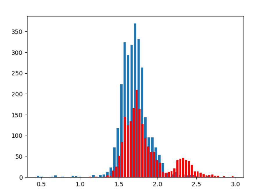
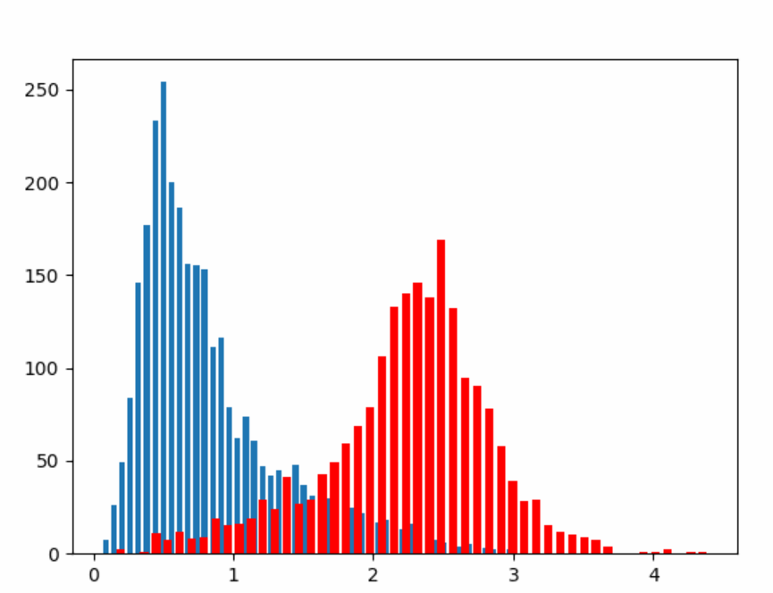
It has been empirically observed that classifiers that capture input semantics do not fit the noise before significantly learning from the clean samples (Arazo et al., 2019). For a classifier trained using a cross entropy loss() on the noisy dataset, this can be exploited to cluster the input samples as being clean/noisy in an unsupervised manner. Initially the training loss on both clean and noisy samples is large, and after a few training epochs, the loss of majority of the clean samples reduces. Since the loss of the noisy samples is still large, this segregates the samples into two clusters with different loss values. On further training, the model over-fits on the noisy samples and the training loss on both samples reduces. We illustrate this in Fig. 2(a)(c). We fit a 2-component Beta mixture model (BMM) over the normalized training losses () obtained after training the model for some warmup epochs . Using a Beta mixture model works better than using a Gaussian mixture model as it allows for asymmetric distributions and can capture the short left-tails of the clean sample losses. For a sample with normalized loss , the BMM is given by:
where denotes the gamma distribution and are the parameters corresponding to the individual clean/noisy Beta distributions. The mixture coefficients and , and parameters () are learnt using the EM algorithm. On fitting the BMM , for a given input with a normalized loss , we denote the posterior probability of having a clean label by:
3.2. Learning and
We aim to train such that when given an input, predicts the clean label and predicts the noisy label for this input (if retains the original clean label for this input, then both predict the clean label). Thus for an input having a clean label, we want ; and for an input having a noisy label, we want and to be the clean label for . We jointly train using the de-noising loss proposed below:
| (1) |
The first term trains the cascade jointly using cross entropy between and . The second term trains to predict correctly for samples believed to be clean, weighted by . Here is a parameter that controls the trade-off between the two terms.
By jointly training with , we implicitly constrain the label noise in . We use an alternative loss formulation by replacing the Bernoulli with the indicator . For ease of notation, we refer the former (using ) as the soft de-noising loss and the latter as the hard de-noising loss .
Thus we use the following 3-step approach to learn and :
-
(1)
Warmup: Train using .
-
(2)
Fitting BMM: Fit a 2-component BMM on the for all .
-
(3)
Training with : Jointly train and end-to-end using .
We summarize our methodology in Algorithm 1, when using .
| Dataset | Num. Classes | Train | Validation | Test |
|---|---|---|---|---|
| TREC (Li and Roth (2002)) | 6 | 4949 | 503 | 500 |
| AG-News (Gulli (2005)) | 4 | 112000 | 8000 | 7600 |
| Model | Token (How/What) based | Length based | |||||||||||
|---|---|---|---|---|---|---|---|---|---|---|---|---|---|
| Noise % | 10 | 20 | 30 | 40 | 50 | 10 | 20 | 30 | 40 | 50 | |||
| word LSTM | Baseline | 89.2 (-0.4) | 84.4 (-8.2) | 77.8 (-10.6) | 76 (-17) | 71.8 (-15.8) | 91.4 (-1.0) | 87 (0.6) | 82.2 (1.8) | 82.4 (-2.6) | 74.2 (-3.0) | ||
| 91.8 (0) | 87.4 (-2.2) | 84.2 (0.4) | 79 (1) | 67.8 (1.4) | 91.6 (-0.6) | 90.2 (-0.8) | 87.4 (-0.2) | 87.4 (-0.8) | 79 (0) | ||||
| 91.8 (0.2) | 90.6 (-1.2) | 83.8 (-6.8) | 79.2 (-19.2) | 75.6 (-15.8) | 92 (0.4) | 90.6 (1) | 85.4 (0.2) | 84 (-2.8) | 75 (-3) | ||||
| word CNN | Baseline | 90.4 (-3.6) | 83.8 (-1.8) | 82.4 (-7.4) | 78.8 (-17.2) | 52 (1.4) | 91 (0) | 88 (1.2) | 85.2 (-1.2) | 82 (-2.6) | 73.6 (-1.4) | ||
| 90 (0.8) | 86.6 (-3) | 84.4 (-0.6) | 80.6 (-4.2) | 74 (-7.6) | 90.6 (-0.8) | 89.6 (-1) | 87.2 (-0.2) | 82.6 (-0.4) | 77 (-6.2) | ||||
| 91.2 (-0.4) | 86.8 (-1.8) | 84.2 (-4.2) | 81.8 (-12) | 65.2 (-12.4) | 92.8 (-3.6) | 91 (-2.2) | 86.8 (-1.4) | 86 (-4) | 75.4 (1.8) | ||||
4. Evaluation
Datasets We experiment with two popular text classification datasets: (i) TREC question-type dataset (Li and Roth, 2002), and (ii) AG-News dataset (Gulli, 2005) (Table 2). We inject noise in the training and validation sets, while retaining the original clean test set for evaluation. Note that collecting real datasets with known patterns of label noise is a challenging task, and out of the scope of this work. We artificially inject noise in clean datasets, which enables easy and extensive experimentation.
Models We conduct experiments on two popular model architectures: word-LSTM (Hochreiter and Schmidhuber, 1997) and word-CNN (Kim, 2014). For word-LSTM, we use a 2-layer BiLSTM with hidden dimension of 150. For word-CNN, we use 300 kernel filters each of size 3, 4 and 5. We use the pre-trained GloVe embeddings (Pennington et al., 2014) for initializing the word embeddings for both models. We train models on TREC and AG-News for 100 and 30 epochs respectively. We use an Adam optimizer with a learning rate of and a dropout of during training. For the noise model , we use a simple 2-layer feedforward neural network, with the number of hidden units . We choose the inputs to the noise model as per the class of label noise, which we describe in Section 4.1 and 4.2. We conduct hyper-parameter tuning for the number of warmup epochs and using grid search over the ranges of {6,10,20} and {2,4,6,8,10} respectively.
Metrics and Baseline We evaluate the robustness of the model to label noise on two fronts: (i) how well it performs on clean data, and (ii) how much it over-fits the noisy data. For the former, we report the test set accuracy (denoted by Best) corresponding to the model with best validation accuracy . For the latter, we examine the gap in test accuracies between the Best, and the Last model (after last training epoch). We evaluate our approach against only training (as the baseline), for two types of noise: random and input-conditional, at different noise levels.
4.1. Results: Random Noise
For a specific Noise %, we randomly change the original labels of this percentage of samples. Since the noise function is independent of the input, we use logits from as the input to . We report the Best and (Last - Best) test accuracies in Table 1. From the experiments, we observe that:
(i) and almost always outperforms the baseline across different noise levels. The performance of and are similar. We observe that training with tends to be better at low noise %, whereas tends to be better at higher noise %. Our method is more effective for TREC than AG-News, since even the baseline can learn robustly on AG-News.
(ii) Our approach using and drastically reduces over-fitting on noisy samples (visible from small gaps between Best and Last accuracies). For the baseline, this gap is significantly larger, especially at high noise levels, indicating over-fitting to the label noise. For example, consider word-LSTM on TREC at 30% noise: while the baseline suffers a sharp drop of 24.8 points from 79.6%, the accuracy of the model drops just 1.0% from 83.4%.

We further demonstrate that our approach avoids over-fitting, thereby stabilizing the model training by plotting the test accuracies across training epochs in Fig. 3. We observe that the baseline model over-fits the label noise with more training epochs, thereby degrading test accuracy. The degree of over-fitting is greater at higher levels of noise (Fig. 3(b) vs Fig. 3(a)). In comparison, our de-noising approach using both and does not over-fit on the noisy labels as demonstrated by stable test accuracies across epochs. This is particularly beneficial when operating in a few-shot setting where one does not have access to a validation split that is representative of the test split for early stopping.
| Noise | AP (7.8%) | Reuters (10.8%) | Either (18.6%) | |
|---|---|---|---|---|
| word LSTM | Baseline | 82.8 (-0.5) | 85.6 (-0.8) | 75.7 (-0.4) |
| 82.7 (0) | 85.7 (-0.1) | 76.6 (-0.4) | ||
| 82.8 (0.3) | 85.5 (0.1) | 76 (-0.1) | ||
| word CNN | Baseline | 83.1 (-0.2) | 85.7 (0) | 76.6 (-0.9) |
| 82.4 (0.8) | 86.2 (0) | 76.1 (0.1) | ||
| 82.5 (0.5) | 86.1 (0.1) | 76.4 (0) |
4.2. Results: Input-Conditional Noise
We heuristically condition the noise function on lexical and syntactic input features. We are the first to study such label noise for text inputs, to our knowledge. For both the TREC and AG-News, we condition on syntactic features of the input: (i) The TREC dataset contains different types of questions. We selectively corrupt the labels of inputs that contain the question words ‘How’ or ‘What’ (chosen based on occurrence frequency). For texts starting with ‘How’ or ‘What’, we insert random label noise (at different levels). We also consider conditional on the text length (a lexical feature). More specifically, we inject random label noise for the longest x% inputs in the dataset. (ii) The AG-News dataset contains news articles from different news agency sources. We insert random label noise for inputs containing the token ‘AP’, ‘Reuters’ or either one of them. We concatenate the contextualised input embedding from the penultimate layer of and the logits corresponding to as the input to . We present the results in Tables 3 and 4.
On TREC, our method outperforms the baseline for both the noise patterns we consider. For the question-length based noise, we observe the same trend of outperforming at high noise levels, and vice-versa. On AG-News, the noise % for inputs having the specific tokens ’AP’ and ’Reuters’ are relatively low, and our method performs at par or marginally improves over the baseline performance. Interestingly, the input–conditional noise we consider makes effective learning very challenging, as demonstrated by significantly lower Best accuracies for the baseline model than for random noise. As the classifier appears to overfit to the noise very early during training, we observe relatively smaller gaps between Best and Last accuracies. Compared to random noise, our approach is less efficient at alleviating the (Best-Last) accuracy gap for input-conditional noise. These experiments however reveal promising preliminary results on learning with input-conditional noise.
5. Conclusion
We have presented an approach to improve text classification when learning from noisy labels by jointly training a classifier and a noise model using a de-noising loss. We have evaluated our approach on two text classification tasks. demonstrate its effectiveness through an extensive evaluation. Future work includes studying more complex for other NLP tasks like language inference and QA.
References
- (1)
- Agarwal et al. (2007) Sumeet Agarwal, Shantanu Godbole, Shourya Roy, and Diwakar Punjani. 2007. How much noise is too much: A study in automatic text classification. In In Proc. of ICDM.
- Arazo et al. (2019) Eric Arazo, Diego Ortego, Paul Albert, Noel O’Connor, and Kevin Mcguinness. 2019. Unsupervised Label Noise Modeling and Loss Correction. In Proceedings of the 36th International Conference on Machine Learning (Proceedings of Machine Learning Research, Vol. 97), Kamalika Chaudhuri and Ruslan Salakhutdinov (Eds.). PMLR, Long Beach, California, USA, 312–321. http://proceedings.mlr.press/v97/arazo19a.html
- Ardehaly and Culotta (2018) Ehsan Ardehaly and Aron Culotta. 2018. Learning from noisy label proportions for classifying online social data. Social Network Analysis and Mining 8 (12 2018). https://doi.org/10.1007/s13278-017-0478-6
- Frénay and Verleysen (2014) Benoît Frénay and Michel Verleysen. 2014. Classification in the Presence of Label Noise: A Survey. IEEE Transactions on Neural Networks and Learning Systems 25 (2014), 845–869.
- Goodman et al. (2016) James Goodman, Andreas Vlachos, and Jason Naradowsky. 2016. Noise reduction and targeted exploration in imitation learning for Abstract Meaning Representation parsing. In Proceedings of the 54th Annual Meeting of the Association for Computational Linguistics (Volume 1: Long Papers). Association for Computational Linguistics, Berlin, Germany, 1–11. https://doi.org/10.18653/v1/P16-1001
- Gulli (2005) A. Gulli. 2005. The Anatomy of a News Search Engine. In Special Interest Tracks and Posters of the 14th International Conference on World Wide Web (Chiba, Japan) (WWW ’05). Association for Computing Machinery, New York, NY, USA, 880–881.
- Hochreiter and Schmidhuber (1997) Sepp Hochreiter and Jürgen Schmidhuber. 1997. Long Short-Term Memory. Neural Comput. 9, 8 (Nov. 1997), 1735–1780. https://doi.org/10.1162/neco.1997.9.8.1735
- Ipeirotis et al. (2010) Panagiotis G. Ipeirotis, Foster Provost, and Jing Wang. 2010. Quality Management on Amazon Mechanical Turk. In Proceedings of the ACM SIGKDD Workshop on Human Computation (Washington DC) (HCOMP ’10). Association for Computing Machinery, New York, NY, USA, 64–67. https://doi.org/10.1145/1837885.1837906
- Jiang et al. (2019) Junjun Jiang, Jiayi Ma, Zheng Wang, Chen Chen, and Xianming Liu. 2019. Hyperspectral Image Classification in the Presence of Noisy Labels. IEEE Transactions on Geoscience and Remote Sensing 57 (2019), 851–865.
- Jiang et al. (2018) Lu Jiang, Zhengyuan Zhou, Thomas Leung, Li-Jia Li, and Li Fei-Fei. 2018. MentorNet: Learning Data-Driven Curriculum for Very Deep Neural Networks on Corrupted Labels. In Proceedings of the 35th International Conference on Machine Learning, Jennifer Dy and Andreas Krause (Eds.). PMLR. http://proceedings.mlr.press/v80/jiang18c.html
- Jindal et al. (2019) Ishan Jindal, Daniel Pressel, Brian Lester, and Matthew Nokleby. 2019. An Effective Label Noise Model for DNN Text Classification. In Proceedings of North American Chapter of the Association of Computational Linguistics 2019.
- Joshi et al. (2014) Aditya Joshi, Abhijit Mishra, Nivvedan Senthamilselvan, and Pushpak Bhattacharyya. 2014. Measuring Sentiment Annotation Complexity of Text. In Proceedings of the 52nd Annual Meeting of the Association for Computational Linguistics (Volume 2: Short Papers). Association for Computational Linguistics, Baltimore, Maryland.
- Kim (2014) Yoon Kim. 2014. Convolutional Neural Networks for Sentence Classification. In Proceedings of the 2014 Conference on Empirical Methods in Natural Language Processing, EMNLP 2014. 1746–1751.
- Larson et al. (2019) Stefan Larson, Anish Mahendran, Andrew Lee, Jonathan K. Kummerfeld, Parker Hill, Michael A. Laurenzano, Johann Hauswald, Lingjia Tang, and Jason Mars. 2019. Outlier Detection for Improved Data Quality and Diversity in Dialog Systems. In Proceedings of the 2019 Conference of the North American Chapter of the Association for Computational Linguistics: Human Language Technologies, Volume 1 (Long and Short Papers). Association for Computational Linguistics, Minneapolis, Minnesota, 517–527. https://doi.org/10.18653/v1/N19-1051
- Li and Roth (2002) Xin Li and Dan Roth. 2002. Learning Question Classifiers. In Proceedings of the 19th International Conference on Computational Linguistics - Volume 1 (Taipei, Taiwan) (COLING ’02). Association for Computational Linguistics, Stroudsburg, PA, USA, 1–7.
- Malik and Bhardwaj (2011) H. H. Malik and V. S. Bhardwaj. 2011. Automatic Training Data Cleaning for Text Classification. In 2011 IEEE 11th International Conference on Data Mining Workshops. 442–449.
- Pennington et al. (2014) Jeffrey Pennington, Richard Socher, and Christopher D. Manning. 2014. GloVe: Global Vectors for Word Representation. In Empirical Methods in Natural Language Processing (EMNLP). 1532–1543. http://www.aclweb.org/anthology/D14-1162
- Reed et al. (2015) Scott E. Reed, Honglak Lee, Dragomir Anguelov, Christian Szegedy, Dumitru Erhan, and Andrew Rabinovich. 2015. Training Deep Neural Networks on Noisy Labels with Bootstrapping.. In ICLR (Workshop), Yoshua Bengio and Yann LeCun (Eds.). http://dblp.uni-trier.de/db/conf/iclr/iclr2015w.html#ReedLASER14
- Thulasidasan et al. (2019) Sunil Thulasidasan, Tanmoy Bhattacharya, Jeff Bilmes, Gopinath Chennupati, and Jamal Mohd-Yusof. 2019. Combating Label Noise in Deep Learning using Abstention. In Proceedings of the 36th International Conference on Machine Learning, Kamalika Chaudhuri and Ruslan Salakhutdinov (Eds.). PMLR. http://proceedings.mlr.press/v97/thulasidasan19a.html
- Wang et al. (2018) Fei Wang, Liren Chen, Cheng Li, Shiyao Huang, Yanjie Chen, Chen Qian, and Chen Change Loy. 2018. The Devil of Face Recognition is in the Noise. arXiv preprint arXiv:1807.11649 (2018).
- Zhan et al. (2019) Xueying Zhan, Yaowei Wang, Yanghui Rao, and Qing Li. 2019. Learning from Multi-Annotator Data: A Noise-Aware Classification Framework. ACM Trans. Inf. Syst. 37, 2, Article 26 (Feb. 2019), 28 pages. https://doi.org/10.1145/3309543
- Zhang et al. (2016) Chiyuan Zhang, Samy Bengio, Moritz Hardt, Benjamin Recht, and Oriol Vinyals. 2016. Understanding deep learning requires rethinking generalization. ICLR (2016). http://arxiv.org/abs/1611.03530 cite arxiv:1611.03530Comment: Published in ICLR 2017.
- Zhang et al. (2018) Hongyi Zhang, Moustapha Cisse, Yann N. Dauphin, and David Lopez-Paz. 2018. mixup: Beyond Empirical Risk Minimization. In International Conference on Learning Representations. https://openreview.net/forum?id=r1Ddp1-Rb
- Zlateski et al. (2018) Aleksandar Zlateski, Ronnachai Jaroensri, Prafull Sharma, and Fredo Durand. 2018. On the Importance of Label Quality for Semantic Segmentation. In CVPR. 1479–1487. https://doi.org/10.1109/CVPR.2018.00160