Towards Reliable Medical Image Segmentation by utilizing Evidential Calibrated Uncertainty
Abstract
Medical image segmentation is critical for disease diagnosis and treatment assessment. However, concerns regarding the reliability of segmentation regions persist among clinicians, mainly attributed to the absence of confidence assessment, robustness, and calibration to accuracy. To address this, we introduce DEviS, an easily implementable foundational model that seamlessly integrates into various medical image segmentation networks. DEviS not only enhances the calibration and robustness of baseline segmentation accuracy but also provides high-efficiency uncertainty estimation for reliable predictions. By leveraging subjective logic theory, we explicitly model probability and uncertainty for the problem of medical image segmentation. Here, the Dirichlet distribution parameterizes the distribution of probabilities for different classes of the segmentation results. To generate calibrated predictions and uncertainty, we develop a trainable calibrated uncertainty penalty. Furthermore, DEviS incorporates an uncertainty-aware filtering module, which utilizes the metric of uncertainty-calibrated error to filter reliable data within the dataset. We conducted validation studies to assess both the accuracy and robustness of DEviS segmentation, along with evaluating the efficiency and reliability of uncertainty estimation. These evaluations were performed using publicly available datasets including ISIC2018, LiTS2017, and BraTS2019. Additionally, two potential clinical trials are being conducted at Johns Hopkins OCT, Duke-OCT-DME, and FIVES datasets to demonstrate their efficacy in filtering high-quality or out-of-distribution data. Our code has been released in https://github.com/Cocofeat/DEviS.
keywords:
Uncertainty estimation , Medical image segmentation , Foundational model1 Introduction
Medical image segmentation, benefit from deep learning techniques, has ushered in a paradigm shift in quantitative pathological assessments [49, 5], diagnostic support systems [51, 52], and tumor analysis [50, 2, 37]. In response to identifying reliable medical image segmentation regions, the focus has transcended mere accuracy. A reliable medical image segmentation model assumes a pivotal role in establishing a foundation of trust and confidence between healthcare professionals and patients. It provides efficient pixel-level confidence among healthcare professionals while delivering robust results [25]. In addition to strive for a closer alignment of network outputs with the ground truth, a reliable model also focuses on delivering accurate and well-calibrated predictions. This allows the model to provide indications of when its output can be trusted, effectively avoiding situations where the model produces overconfident predictions [10, 38, 28]. Significantly, the reliable model provides timely warnings when confronted with data high uncertainty, thereby recognizing the potential limitations and reliability of its predictions [24]. With this paper, we embark on a journey to develop a reliable foundational model for medical image segmentation, facilitating robust segmentation and confident region identification. By employing calibrated uncertainty estimation and validating partial clinical applications, our ultimate aim is to foster trust between healthcare professionals and deep learning models.
In recent years, remarkable advancements have been achieved in the endeavor to enhance the accuracy of deep network architectures for medical image segmentation. Fully Convolutional Networks (FCN) have been developed to achieve end-to-end semantic segmentation with impressive results [27]. Based on FCN, the U-Net [7] model and its variants [55, 3, 36, 31] were proposed to improve feature representations and segmentation outcomes. More recently, highly expressive transformers [44, 6, 26, 54] have gained success in computer vision and medical image segmentation. While existing researches limit medical image segmentation performance development by solely emphasizing segmentation accuracy. The limitations come from two aspects: 1) The aforementioned backbones for medical image segmentation neglect the presence of ambiguous decisions that AI systems may make. There are instances where AI decisions lack informed judgment, necessitating principled methods to quantify uncertainty for clinical application. 2) Fundamental frameworks for medical image segmentation have limitations in handling noise perturbations in data and detecting high uncertainty samples, which are crucial for real-world deployment [25].
Uncertainty estimation methods play a pivotal role in assessing model confidence. According to [56], uncertainty quantification in medical domain includes Bayesian [19, 39] and non-Bayesian [45, 22, 28, 40, 43, 14, 34] based methods. Bayesian-based methods [19, 29] enables the segmentation networks to learn a distribution over the model parameters with uncertainty, which are computationally expensive [8]. Monte Carlo Dropout-based methods [35] alleviate this problem by introducing dropout to approximate uncertainty from multiple predictions. Non-Bayesian based methods have been developed, which mainly include test time augmentation (TTA) [45], deep ensemble (DE) [22], deterministic [34], and evidential [40, 14, 47] based methods. In this paper, we focus on evidence-based deep learning methods [40] applied to medical image segmentation, aiming to provide accurate and reliable segmentation. As depicted in Fig. 1 (a), traditional medical image segmentation only offers approximate segmentation results without providing uncertainty measures for each pixel. Consequently, when encountering anomalous samples such as noise, its segmentation performance deteriorates, failing to indicate which pixels are reliable. Illustrated in Fig. 1 (b), ensemble-based medical image segmentation methods train multiple models to produce multiple predictions for obtaining average prediction results and uncertainty. However, this method incurs high training costs for uncertainty estimation and yields poorer results under noisy samples. Popular uncertainty estimation methods such as Monte Carlo Dropout [35] and probability-based methods [19] inevitably alter network structures and incur computational costs. In contrast, the reliable medical image segmentation method proposed in this paper, as shown in Fig. 1 (c), not only provides robust segmentation results but also offers uncertainty estimations for each pixel. Moreover, this uncertainty estimation only requires one forward pass, significantly enhancing computational efficiency. Additionally, previous research primarily focused on utilizing uncertainty to improve segmentation performance, overlooking the crucial aspect of model calibration. However, well-calibrated models align their predictions with the true probabilities of outcomes, thereby enhancing the reliability of model predictions in medical diagnosis [20]. Therefore, this paper also proposes an approach that combines efficient uncertainty estimation and model calibration to identify reliable medical image segmentation regions. Lastly, unlike the aforementioned uncertainty estimation methods, which are less utilized in healthcare for clinical applications, this paper extends the proposed method to filtering out-distribution data and indicating high quality data.

In this study, we present a Deep Evidential Segmentation model (DEviS) for identifying reliable medical image segmentation regions that seamlessly integrates with existing base frameworks, offering efficient confidence assessment, robustness, and well-calibrated results. Our work also explores the potential of DEviS in clinical applications. The key contributions of this study are threefold: 1) we derive probabilities and uncertainties for different class segmentation problems via Subjective Logic (SL) theory, where the Dirichlet distribution parameterizes the distribution of probabilities for different classes of the segmentation results. 2) we develop a trainable calibrated uncertainty penalty (CUP) to generate more calibrated confidence and maintain the segmentation performance of the base network. 3) we develop an uncertainty-aware filtering (UAF) strategy to facilitate the translation of DEviS into clinical applications. This strategy enables the detection of OOD data and provides insights into image data quality. It was validated using three clinical public datasets for the aforementioned strategy. 4) We conducted extensive experiments on three publicly available datasets: ISIC2018, LiTS2017, and BraTS2019. Our objective was to verify the accuracy and robustness of the model in predicting standard and adversarial samples, which include noise, blurred, and randomly masked, while also assessing the efficiency and reliability of uncertainty estimation. To reiterate, we establish an easily portable framework towards achieving reliable medical image segmentation.
Compared to the previous conference version [57], we have implemented significant enhancements in the following areas: 1) We introduced a trainable calibrated uncertainty penalty to generate more reliable confidence, thereby preserving the segmentation performance of the base network. 2) We devised an UAF strategy to facilitate the integration of DEviS into clinical applications. 3) We conducted clinical applications involving OOD data detection and image data quality indicators from the perspective of segmentation uncertainty. 4) We performed extensive experiments on diverse datasets to validate the robustness of our model.
2 Related work
In this section, we first briefly review deep learning works for medical image segmentation. Then, different uncertainty quantification methods and its application in medical image segmentation are introduced, respectively.
2.1 Deep learning methods for medical image segmentation
In last years, most methods used for medical image segmentation were based on Convolutional Neural Networks (CNNs). Attributed to the elegant design of skip connections in U-Net [7, 15], a similar structure V-Net was presented for 3D image segmentation based on a volumetric. Then, other U-Net variants [53, 36] focused on getting better feature representations about the targets. The representative Attention-UNet employed attention gates in the skip connection to increasing the model sensitivity for varying shapes and sizes of organs/tumors. Zhou et al. [55] further rethinked the skip connections and optimal depth of the U-Net and presented UNet++ for semantic and instance segmentation. Currently, the success of Transformer [44] in image classification has received attention in the field of medical image segmentation. TransUNet+ [26] applied Vision Transformer [6] for medical image segmentation, introducing redesigned skip connections to enhance skip features and improve global attention. Wang et al. [48] developed the Transformer for brain tumor segmentation based on 3D CNN immediately. Moreover, Zhou et al. present nnFormer [54], a 3D transformer designed specifically for volumetric medical image segmentation. In addition to utilizing a fusion of interleaved convolution and self-attention operations, nnFormer introduces a self-attention mechanism that operates both locally and globally within the image volumes. Despite the increasing number of works leveraging various deep learning models to enhance the accuracy of medical image segmentation, clinicians are eager to understand the reliability of segmentation results. Meanwhile, these models seldom achieve robust predictions under noisy conditions.
2.2 Uncertainty quantification and its application in medical image segmentation.
Recently, uncertainty quantification has been widely investigated for many existing medical image segmentation tasks. Non-Bayesian methods include dropout-based [35], deep ensemble-based [28], and deterministic-based [34] are widely circulated for the medical image segmentation. Wang et al. [45] proposed a test-time augmentation-based aleatoric uncertainty for brain tumor segmentation by Monte Carlo sampling. Mehrtash et al. [28] presented model ensembling for confidence calibration of the FCNs. Mukhoti et al. [34] extend the deep deterministic uncertainty method [33] using feature space densities for the semantic segmentation. Besides, Bayesian approaches including Variational inference methods [19, 1] are proposed to estimate the uncertainty of medical images. To gain uncertainty from a large number of plausible hypotheses, Kohl et al. [19] associated U-Net with a conditional variational autoencoder. They compared it with other outperformed the existing methods, such as U-Net Dropout and U-Net ensemble on a lung abnormality segmentation task. Although the above methods quantify the uncertainty of medical image segmentation, they prioritize more accurate segmentation results over obtaining calibrated uncertainty and robust segmentation results. More importantly, these methods may require significant changes to the network structure, making them less adaptable to integration into arbitrary network architectures, and involving excessive additional computations during the uncertainty estimation process.
3 Proposed method
In our proposed DEviS model, we employ an arbitrary network structure as the backbone network for extracting deep evidential features, which can be U-Net [7, 15], its variants [31, 36], or transformer-based methods [54]. To address the issue of over-confidence, DEviS utilizes the softplus activation function layer instead of the softmax layer. Additionally, it utilizes the Dirichlet distribution to generate a predictive distribution rather than a single output, enhancing the reliability of the segmentation results [40]. Furthermore, SL [16] is incorporated to establish probability and uncertianty for different segmentation classes, enabling evidential uncertainty estimation. To enhance the reliability of model predictions in medical diagnosis, a specifically designed CUP for well-calibrated medical image segmentation is developed. Moreover, a UAF strategy is devised to facilitate subsequent clinical tasks by detecting and indicating medical data with its uncertainty. Ultimately, a comprehensive training loss function is formulated, encompassing medical image segmentation, uncertainty estimation, and uncertainty calibration, to ensure reliable medical image segmentation.


3.1 Constructing DEviS
1) Deep evidential feature extraction. U-Net [7, 15], its variants [31, 36] and transformer [54] have seen recent widespread used across medical image modalities. We thus employed one of them as our backbone for capturing contextual information. For U-Net based methods, the backbones only performed down-sampling three times to achieve a balance between GPU memory usage and segmentation accuracy. For the transformer-based method, we follow its design [54]. DEviS can freely choose any backbone to extract image features. We only use its decoder output feature vector without the softmax layer. For a random image in a medical image domain , this process can be defined as:
| (1) |
Where is any network backbone without the softmax layer. In this study, we assessed the performance of the different general backbones (U-Net [7], V-Net [31], Attention-UNet [36], nnU-Net [15]) and nnformer [54]. For typical medical image segmentation tasks [9, 23, 48], the predictions are usually carried by the softmax layer as the final layer. As mentioned in [43, 12], the softmax layer has a tendency to display high confidence even for wrong predictions. DEviS mitigates this issue by utilizing the softplus activation function layer instead of the softmax layer. Therefore, following the output of any neural network, a softplus activation function layer () is applied to ensure that the network output is non-negative, which is considered as evidence for the backbone feature output.
| (2) |
2) Dirichlet distribution for medical image segmentation. We then obtain a Dirichlet distribution from the network output, which is considered as the conjugate prior of the multinomial distribution [16]. This provides a predictive distribution for medical image segmentation and derives uncertainty from this distribution. For , the projected probability distribution of multinomial opinions is defined by:
| (3) |
where , and are the belief mass distribution, base rate distribution and the uncertainty mass distribution over , respectively. Here, the variable x represents any dimensionality medical image, including two-dimensional, three-dimensional, or even multi-dimensional images. Then, Dirichlet PDF can be used to represent probability density over , which is given by:
| (4) |
where Dirichlet distribution with parameters is considered as basic belief assignment. is the -dimensional multinomial beta function, and is the C-dimensional unit simplex, given by:
| (5) |
The total strength can be denoted as:
| (6) |
denotes the weight of the base rate distribution . To simplify equations (1) and (4), we consider the base rate distribution to be and to be . That is .
3) Evidential uncertainty estimation. One of the generalizations of Bayesian theory for subjective probability is the Dempster-Shafer Theory (DST) [4]. The Dirichlet distribution is formalized as the belief distribution of DST over the discriminative framework in the SL [16]. For medical image segmentation, we define the DEviS framework through SL [16], which derives the probability and uncertainty of different class segmentation problem based on deep evidential features. In Fig. 1(a), we illustrate the uncertainty estimation process 3D -class medical image segmentation task. Given a 3D image input and evidential feature output , where , denotes the evidence for -th class. The SL provides a belief mass and an uncertainty mass for different classes of segmentation results. The mass values are all non-negative and their sum is one. Specifically, for the -th pixel, it has the following definition:
| (7) |
where and denote the probability of the -th pixel for the -th class and the overall uncertainty of the -th pixel in , respectively, where and . SL then associates the evidence having the Dirichlet distribution with the parameters , where and . After that, the belief mass and the uncertainty of the -th pixel can be denoted as:
| (8) |
where denotes the Dirichlet strength. The more evidence of the -th class obtained by the -th pixel, the greater its probability. Vice versa.
For clarity, we provide a example that demonstrates the formulation in the context of a three-category 3D medical image segmentation task. Let us consider the evidence output for the -th pixel. The corresponding Dirichlet distribution parameter is . In accordance with the SL theory [16], the three categories of subjective opinions are represented by , , and , respectively. Additionally, the uncertainty mass is given by . Hence, the point on the simplex represents the opinions of the -th pixel as . This observation indicates that there is a significant amount of evidence supporting the classification of the -th pixel as the first class, with an associated uncertainty value of 0.067 for the pixel. This formulation can be extended to all pixels in , allowing the estimation of the confidence for each individual pixel. The subjective opinion of image is then obtained as .
4) Calibrated uncertainty penalty. Though DEviS provides a means for directly learning evidential uncertainty without sampling, the uncertainty might not be totally calibrated to enhance the reliability of model predictions. As pointed out in [32, 20], a reliable and well-calibrated model should be uncertain in its predictions when being inaccurate, and be confident for the opposite case. Also, calibrated uncertainty will also help in detecting the OOD data to caution AI researchers. More importantly, our CUP relied on the theoretically sound loss-calibrated approximate inference framework [21] as utility-dependent penalty term for obtaining well-calibrated uncertainty in medical domain. To this end, this paper introduces a loss function called CUP, which considers the relationship between accuracy and uncertainty in medical image segmentation. This is an optimization method used to calibrate uncertainty, aiming to maintain lower uncertainty for accurate predictions and higher uncertainty for inaccurate predictions during the training process, thereby achieving well-calibrated uncertainty. This enables the backbone to improve segmentation performance, in addition to learn to provide well-calibrated uncertainty. The CUP is defined as:
| (9) |
where , , and denote the number of samples for the network output category of Accurate and Certain (A&C), Accurate and Uncertain (A&U), the Inaccurate and Certain (I&C) and the Inaccurate and Uncertain (I&U), respectively (Examples of probability simplex can be seen in Fig. 2 b). We define proxy functions to approximate them as given by:
| (10) |
Ideally, we anticipate the model to exhibit certainty in its predictions when accurate, and to yield high uncertainty estimates when making inaccurate predictions. Therefore, we encourage DEviS to learn more A&C samples in the early training period and provide more I&U samples later in training. Correspondingly, we seek to impose penalties on I&C samples during the initial phase of training and on A&U samples during the later stage (Training process of CUP can be seen in Fig. 2 b). Following [20], we propose an uncertainty calibration loss function in Eq. 20. More details about the training process of calibrated uncertainty and uncertainty calibration loss are presented in B.
3.2 Uncertainty-aware filtering
To apply DEviS to clinical tasks to screen out reliable data, we propose a Uncertainty award filtering strategy (Fig. 2 c). This will benefit the predictive accuracy of ID and OOD data. According to [10], a well-calibrated with confidence reflects the reliability of the model. Inspired by this, We first formulate an Uncertainty-based Calibration Error (UCE) to judge the reliability of the data according to the accuracy and uncertainty of the data. For a given validation set and its uncertainty estimation , the UCE of each image can be denoted as follows:
| (11) |
where and denote the accuracy and confidence of the -th image data. The represents the mean value of the uncertainty estimate corresponding to the ground truth of the medical image segmentation. As such, we consider the largest UCE sample to be the tolerable maximum for ID data or high-quality data, expressed as follows:
| (12) |
Therefore, we derive the adaptive uncertainty threshold from the uncertainty distribution of the validation dataset , ensuring the selection of the most reliable threshold. For any OOD or low-quality image of segmentation task, the reliability of the data can be judged according to the following formula:
| (13) |
and denote the unreliable data and reliable data, respectively. It should be noted that for OOD or low-quality data, the model is likely to filter the data it considers reliable or not. Unreliable data may still require further diagnosis by clinical experts.
3.3 Evidential calibrated training loss function
Due to the imbalance of organ/tumor, our DEviS is first trained with cross-entropy loss function, which is defined as:
| (14) |
where and are the label and predicted probability of the -th sample for class . Then, SL associates the Dirichlet distribution with the belief distribution under the framework of evidence theory for obtaining the probability of different classes and uncertainty of different voxels based on the evidence collected from backbone. Therefore, Eq. 14 can be further improved as follows:
| (15) |
where denote the function. is the class assignment probabilities on a simplex. To guarantee that incorrect labels will yield less evidence, even shrinking to 0, the KL divergence loss function is introduced as below:
| (16) |
where is the function. denotes the adjusted parameters of the Dirichlet distribution, which is used to ensure that ground-truth class evidence is not mistaken for 0. Therefore, the evidential deep learning process can be defined as:
| (17) |
where is the balance factor and set to be 0.02 [40]. The gradient Analysis for can be found in A. Furthermore, the Dice score is an important metric for judging the performance of organ/tumor segmentation. Therefore, we use a soft Dice loss to optimize the network, which is defined as:
| (18) |
where and are the label and probability of the target. is the balance factor. So, the segmentation loss function can be define as follows:
| (19) |
Then, according to Sec. 3.1 of calibrated uncertainty penalty, the loss function for well-calibrated uncertainty can be defined as follows:
| (20) |
To guide the model optimization at the early stage of network training, is noted as the annealing factor, which is defined by . and are the total epochs and the current epoch, respectively. The value of is set to 0.01. More loss-calibrated approximate inference framework analysis in CUP loss can be referred to B. Finally, the overall evidential calibrated training loss function of our proposed network can be defined as follows:
| (21) |
4 Experimental results
4.1 Experimental Setup & Datasets
1) Experimental Setup: Our proposed network is implemented in PyTorch and trained on NVIDIA GeForce RTX 2080Ti. We adopt the Adam to optimize the overall parameters. The initial learning rates for different datasets are set to be 0.0002 (ISIC2018), 0.001 (LiTS2017), and 0.002 (BraTS2019). The poly learning strategy is used by decaying each iteration with a power of 0.9. The maximum of the epoch is set to 200. The batch sizes for the lesion segmentation, live segmentation, and brain tumor segmentation are set to 16, 4, and 2. All the following experiments adopted a five-fold cross-validation strategy to prevent performance improvement caused by accidental factors. For the ISIC2018 dataset, we used the data augmentation by random cropping, flipping, and random rotation as same as [9]. For the LiTS2017 dataset, we only used the data augmentation by random flipping. For the BraTS2019 dataset, the data augmentation techniques are similar as [48]. For the clinical application of OOD detection, we conducted the experiments on the Johns Hopkins OCT dataset and the Duke OCT dataset with DME. For the clinical application of data quality indicator, we conducted the experiments on the FIVES dataset. In these applications, the initial learning rate for the dataset are set to be 0.0001. The poly learning strategy is used by decaying each iteration with a power of 0.9. The maximum of the epoch is set to 100. The batch sizes for the layer-segmentation and voxel-segmentation from OCT are set to 8. The following will provide additional detailed information about the ISIC2018, LiTS2017, and BraTS2019 datasets used, as well as information regarding degraded image data. It also elaborates on the datasets utilized in clinical applications.
2) ISIC2018 [42] dataset. First, the public available International Skin Imaging Collaboration (ISIC) 2018 dataset is validated for reliable 2D medical image segmentation task. Following the [9], a total of 2594 images and their ground truth are randomly divided into a training set, validation set, and test set, containing 1814, 260 and 520 images, respectively. To verify the robustness and credibility of different models under OOD conditions, we add different levels of Gaussian noise and random masks to the test set, and perform 5-fold cross-validation for final results. First, we added the standard deviation of the Gaussian noise ranging from [0.1, 0.2, 0.3, 0.4, 0.5] to the original data with normalization. Then, the strategy of random mask with 8 pixel-size like [13] ranging from [0.1, 0.25, 0.4] are deployed for the original data.
3) LiTS2017 [2] dataset. Second, Liver Tumor Segmentation (LiTS) Challenge 2017 is validated for reliable 3D medical image segmentation task. It contains the public 131 and 70 contrast-enhanced 3D abdominal CT scans. Following [23], we resampled the overall samples to the same resolution with the spacing of , and randomly divided them into training set and test set containing 105 (nearly 985 volumes) and 26 cases (nearly 245 volumes), respectively. For the OOD condition, we also add different levels of Gaussian noise, Gaussian blur and random mask to the test data of 3D volumes. Gaussian noise is added to the normalized data with standard deviation of the ranging from [0.05, 0.1, 0.2, 0.3, 0.4]. Gaussian blur is added to the test data with variance varying from 11 to 35 and kernel sizes of 10 to 20, specifically ranging from [(11, 10), (15, 10), (23, 20), (35, 20)]. The strategy of random mask with 8 pixel-size like [13] ranging from [0.1, 0.25, 0.4] are also deployed for the original data.
4) BraTS2019 dataset. More importantly, the Brain Tumor Segmentation (BraTS) 2019 challenge [30] with varying degradation conditions(such as noise, blur and mask) are constructed for reliable multi-modality 3D medical image segmentation tasks. Four modalities of brain MRI scans with a volume of are used. 335 cases of patients on BraTS2019 with ground-truth are randomly divided into train dataset, validation dataset, and test dataset with nearly 265, 35, and 35 cases, respectively. The three tumor sub-compartment labels are combined to segment the whole tumor and all inputs are uniformly adjusted to voxels during the training. The outputs of our network contain 4 classes, which are background (label 0), necrotic and non-enhancing tumor (label 1), peritumoral edema (label 2), and GD-enhancing tumor (label 4). Similarly, in order to verify the reliability uncertainty estimation and robust segmentation results of the model under OOD data, three changes were made to the test set, namely Gaussian noise, Gaussian blur, and random mask. Gaussian noise is added to the normalized data with standard deviation of the ranging from [0.5, 1.0, 1.5, 2.0]. Gaussian blur is added to the test data with variance varying from 3 to 9 and kernel sizes of 3 to 9, specifically ranging from [(3, 3), (5, 5), (7, 7), (9, 9)]. The strategy of random mask with 8 pixel-size like [13] ranging from [0.1, 0.25, 0.4, 0.6] are also deployed for the original data.
5) Johns Hopkins OCT & Duke-OCT-DME datasets. In the first application, Johns Hopkins OCT (JH-OCT) dataset and Duke OCT dataset with Diabetic Macular Edema (Duke-OCT-DME) are used for the OOD detector. 35 cases of patients on JH-OCT with ground-truth are randomly divided into train dataset, validation dataset and test dataset with nearly 25, 5 and 5 cases, respectively. The 5 cases of test dataset on JH-OCT are used for ID detection. In particular, the 10 cases from the Duke-OCT-DME are used as another test dataset for OOD detection. Every case is uniformly adjusted to voxels during the training and testing.
6) FIVES dataset. In the second application, the Fundus Image Vessel Segmentation (FIVES) dataset is used for the quality indicator. In the FIVES dataset, each image was evaluated for four qualities: normal, lighting and color distortion, blurring, and low-contrast distortion. In this experiment, we define normal images as high-quality data and images under other conditions as low-quality data. During the experimental process, DEviS was initially trained on the FIVES dataset, which comprises 300 slices of high-quality images. Subsequently, the performance of DEviS was evaluated on a mixed dataset from FIVES, consisting of 300 slices comprising both high and low-quality images. This mixed dataset comprised 159 high-quality slices and 141 slices of low-quality images. Throughout both the training and testing stages, each case was consistently adjusted to dimensions of voxels, ensuring uniformity across the dataset.
4.2 Compared Methods & Evaluation
1) Compared Methods: In this study, we seamlessly integrated our proposed method into both U-Net-based and transformer-based frameworks to rigorously evaluate its robustness and reliability pre and post-integration. Comparative analyses were conducted against state-of-the-art methods employing uncertainty estimation techniques. The U-Net variants encompassed traditional U-Net [7], V-Net [31], Attention-UNet [36], and nnU-Net [15], while the transformer-based approach was predominantly represented by nnFormer [54]. Additionally, our approach underwent comprehensive comparisons with uncertainty estimation methodologies, including U-Net-based Monte Carlo dropout sampling (DU) [18], U-Net-based ensemble (UE) [22], Probabilistic-UNet (PU) [19], Bayesian QuickNAT (BQNAT) [39], Test-Time Augmentation (TTA) [46] and our conference version [57]. These comparisons were undertaken to elucidate the superiorities and limitations of our proposed method in the context of existing cutting-edge techniques.
2) Evaluation Metrics: The following metrics are employed for quantitative evaluation. (a) The Dice score (Dice) and (b) Average symmetric
surface distance (ASSD) is adopted as an intuitive evaluation of segmentation accuracy. Given the absence of ground truth for the uncertainty estimate, we utilize the same evaluation metrics as referenced in [11, 17] to assess its performance. (c) Expected calibration error (ECE) [11, 17] and (d) Uncertainty-error overlap (UEO) [11, 17] are used as evaluation of uncertainty estimations.
Dice score. Dice measures the overlap areas between the prediction map and ground truth mask . It can be represented by:
| (22) |
ASSD. ASSD calculates the accuracy of segmented boundaries between the point sets of prediction and the point sets of ground truth . It can be defined as:
| (23) |
where represents the minimum Euclidean distance from point to all the points in .
ECE. ECE approximates the calibration gap between confidence [11] and accuracy [11]. It can be expressed as:
| (24) |
where is the number of interval bins. denotes the set of indices of samples whose prediction confidence falls into the interval. means the number of samples. ECE closer to zero means better calibration uncertainty.
UEO. UEO measures the overlap between the segmentation error and the thresholded uncertainty , which can be denoted as:
| (25) |
where a higher UEO (close to one) indicates a better calibration.
4.3 DEviS improves robustness and calibration for different base networks.
To illustrate this, we tackled three challenging medical image segmentation tasks using different datasets: (1) 2D skin lesion images from the ISIC2018 dataset, (2) 3D liver CT images from the LiTS2017 dataset, and (3) multi-modal 3D MRI images from the BraTS2019 dataset. These tasks encompass the segmentation of various tissues and tumors, aiming to achieve accurate and robust segmentation performance across different levels of normal and degraded (noise, blur, and random mask) conditions in medical images, alongside reliable and efficient uncertainty estimation.
4.3.1 DEviS for 2D medical image
We initially enhance the robustness and accuracy of the base network in skin lesion boundary segmentation [42, 9] using DEviS. We conducted studies at different levels of Gaussian noise and random masking based on the ISIC2018 dataset (2D dermoscopic image) to validate the robustness of our proposed framework.
1) Comparison with U-Net based methods. As shown in Fig. 3 (a), the comparison results between DEviS and other U-Net variants under different Gaussian noise levels and mask ratios are presented. Fig. 3 (a) indicates a gradual degradation in performance for U-Net, AU-Net, V-Net, and nnU-Net, particularly at higher mask ratios and noise levels. Upon applying DEviS, the results exhibit a certain degree of robustness to interference. When equipped with DEviS, U-Net demonstrates an average improvement of 10.6% and 8.9% in Dice metric under degraded conditions of Gaussian noise and random masking, respectively. Additionally, the generated uncertainty estimates, as illustrated in Fig. 3 (c), can be utilized by researchers and clinicians to discern the unreliability of the data.
2) Comparison with uncertainty-based methods. As shown in Fig. 3 (a), the comparison results of the ECE and UEO metrics between the proposed method and other uncertainty estimation methods are presented. It reveales that BQNAT, DU, PU, UE, and TTA methods were significantly affected by noise and masking, while the perturbation on U-Net, nnU-Net, and V-Net methods was relatively minor after applying DEviS. A comparison of uncertainty estimation results using ECE and UEO metrics indicated that U-Net, nnU-Net, and V-Net with DEviS achieved better uncertainty estimation. Visualizations of segmentation results and uncertainty estimation as shown in Fig. 3 (c), demonstrate that the proposed DEviS method provides more reliable uncertainty estimation for target edges and the noised or masked pixels.


4.3.2 DEviS for 3D medical image
We further tasked DEviS with enhancing the robustness and accuracy of the base networks in diagnosing hepatocellular diseases [23]. To verify the reliability and robustness of our method, we conducted studies with the Liver2017 dataset (3D CT) under differing levels of Gaussian noise, Gaussian blur, and random masking to achieve robust medical image segmentation.
1) Comparison with U-Net based methods. As shown in Fig. 4 (a), as the degradation conditions worsened, the segmentation results based on U-Net methods exhibited a more pronounced decline in Dice and ASSD metrics. However, this trend could be mitigated by applying the DEviS method. Taking nnU-Net as an example, the robustness was significantly enhanced after integrating the DEviS model under three degradation conditions, with average improvements of 23.7%, 8.6%, and 7.0% in Dice metrics. Similarly, as depicted in Fig. 4 (c), the uncertainty estimation maps generated by the integrated DEviS method can assist physicians in diagnosis and analysis.
2) Comparison with uncertainty-based methods. We repeated the study with uncertainty-based algorithms to further compare the calibrated uncertainty for segmentation. Performance in uncertainty estimation for most uncertainty-based methods degrades with increasing Gaussian noise, Gaussian blur, and random masking (Fig. 4 a). However, the backbones equipped with DEviS mitigates this degradation. Under normal conditions, our framework provides higher uncertainty for liver edges compared to other methods. Under noised conditions, our framework is more sensitive to unseen regions and provides high uncertainty (Fig. 4 c). DEviS thus allows clinicians or annotators to better focus on areas of uncertainty. Please refer to Appendix C Fig S2 for more visual results.


4.3.3 DEviS for Multi-modality 3D medical image
To further validate the robustness and accuracy of the DEviS model in diagnosing brain tumor diseases, experiments were conducted under differing levels of Gaussian noise, Gaussian blur, and random masking. It is worth mentioning that we included the nnFormer model based on the Transformer architecture, which has shown good performance in 3D medical image segmentation, for comparison in this study.
1) Comparison with U-Net and transformer based methods. As shown in Fig. 5 (a), under normal conditions, V-Net, Attention-UNet, nnU-Net, and nnFormer demonstrate comparable performance; however, their segmentation performance begins to degrade under different levels of Gaussian noise, Gaussian blur, and random masking, with the impact becoming more pronounced as the severity increases. The integration of DEviS enhances the robustness under different levels of Gaussian noise, Gaussian blur, and random masking. Taking the Attention-UNet method based on U-Net as an example, the introduction of DEviS results in an average increase of 12.6% and 5.1% in the Dice metric under Gaussian noise and Gaussian blur conditions, respectively. Similarly, considering the nnFormer based on the Transformer, the introduction of DEviS leads to an average increase of 2.21% and 5.93% in the Dice metric under Gaussian noise and random masking conditions, respectively. It is noteworthy that DEviS exhibits superior robustness in uncertainty estimation compared to the conference version of the TBraTS method. Additionally, as depicted in Fig. 5 (c), the segmentation results of different methods show that under Gaussian noise, introducing the DEviS model can slightly improve the segmentation results of nnU-Net and V-Net, while U-Net and Attention-UNet with DEviS demonstrate more robust segmentation results. This is because nnU-Net and V-Net themselves possess certain noise resistance capabilities.
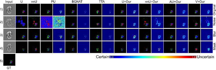
2) Comparison with uncertainty-based methods. Finally, we compared our proposed method with other uncertainty estimation methods on this dataset. As shown in Figs. 5 (a), based on the ECE and UEO metrics, the performance of uncertainty-based methods gradually deteriorates with increasing levels of Gaussian noise, Gaussian blur, and random masking. However, methods integrated with DEviS exhibit slower degradation, especially for UNet, Attention-UNet, and nnFormer. Figs. 5 (c) provides a more intuitive comparison of the uncertainty estimation results for brain tumors among different methods. It is observed that the integrated DEviS-based network architecture provides more reliable uncertainty estimation, manifested in robust segmentation results under both normal and degraded conditions. Additionally, it offers corresponding uncertainty estimations and provides more pronounced uncertainty estimations for pixels affected by noise or masking. Please refer to Appendix C Fig S3 for more visual results.


| Methods | Testing time | Parameter | FLOPs | Dice | ASSD | ECE | UEO | |||||
|---|---|---|---|---|---|---|---|---|---|---|---|---|
| N | OOD | N | OOD | N | OOD | N | OOD | |||||
| ISIC2018 | UE [22] | 13.88 s | 7.77 M | 137.34 G | 0.839 | 0.425 | 8.28 | 30.20 | 0.049 | 0.142 | 0.858 | 0.416 |
| DU [18] | 26.75 s | 7.77 M | 137.34 G | 0.849 | 0.369 | 8.06 | 31.78 | 0.052 | 0.163 | 0.865 | 0.544 | |
| PU [19] | 0.14 s | 27.35 M | 108.54 G | 0.857 | 0.580 | 8.19 | 21.87 | 0.055 | 0.130 | 0.868 | 0.665 | |
| TTA [46] | 26.16 s | 7.77 M | 137.34 G | 0.870 | 0.473 | 7.16 | 27.02 | 0.048 | 0.159 | 0.883 | 0.506 | |
| BQNAT [39] | 6.18 s | 7.77 M | 41.22 G | 0.851 | 0.516 | 7.83 | 32.47 | 0.052 | 0.160 | 0.864 | 0.543 | |
| U+Our | 0.07 s | 7.77 M | 13.74 G | 0.868 | 0.607 | 7.41 | 21.47 | 0.048 | 0.119 | 0.871 | 0.674 | |
| V+Our | 0.08 s | 13.07 M | 15.45 G | 0.874 | 0.781 | 6.71 | 11.35 | 0.045 | 0.087 | 0.905 | 0.839 | |
| nnU+Our | 0.08 s | 7.77 M | 14.13 G | 0.873 | 0.789 | 6.72 | 13.47 | 0.047 | 0.090 | 0.910 | 0.853 | |
| LiTS2017 | UE [22] | 162.02 s | 4.75 M | 776.04 G | 0.856 | 0.603 | 4.57 | 9.58 | 0.031 | 0.077 | 0.858 | 0.647 |
| DU [18] | 170.06 s | 4.75 M | 776.04 G | 0.874 | 0.607 | 3.65 | 8.35 | 0.034 | 0.093 | 0.880 | 0.670 | |
| PU [19] | 1.32 s | 5.13 M | 157.46 G | 0.938 | 0.690 | 0.92 | 8.45 | 0.017 | 0.086 | 0.941 | 0.703 | |
| TTA [46] | 166.55 s | 4.75 M | 108.54 G | 0.827 | 0.536 | 4.99 | 31.59 | 0.040 | 0.101 | 0.839 | 0.158 | |
| BQNAT [39] | 48.84 s | 4.75 M | 108.54 G | 0.809 | 0.487 | 5.44 | 17.77 | 0.054 | 0.138 | 0.815 | 0.207 | |
| U+Our | 0.73 s | 4.75 M | 77.60 G | 0.933 | 0.800 | 1.27 | 4.29 | 0.020 | 0.047 | 0.935 | 0.842 | |
| V+Our | 0.35 s | 2.31 M | 48.01 G | 0.944 | 0.797 | 0.93 | 4.41 | 0.017 | 0.049 | 0.949 | 0.825 | |
| nnU+Our | 0.90 s | 16.55 M | 264.19 G | 0.946 | 0.773 | 0.84 | 4.37 | 0.016 | 0.044 | 0.952 | 0.846 | |
| BraTS2019 | UE [22] | 1626.80 s | 4.76 M | 6941.65 G | 0.857 | 0.709 | 3.42 | 4.93 | 0.0091 | 0.0211 | 0.857 | 0.727 |
| DU [18] | 1428.30 s | 4.76 M | 6941.65 G | 0.825 | 0.662 | 2.50 | 5.79 | 0.0062 | 0.0104 | 0.855 | 0.697 | |
| PU [19] | 15.40 s | 5.13 M | 1423.74 G | 0.864 | 0.470 | 1.73 | 10.02 | 0.0058 | 0.0143 | 0.874 | 0.622 | |
| TTA [46] | 1230.09 s | 4.76 M | 6941.65 G | 0.841 | 0.682 | 2.54 | 5.58 | 0.0064 | 0.0112 | 0.848 | 0.717 | |
| BQNAT [39] | 714.72 s | 4.76 M | 2082.50 G | 0.846 | 0.681 | 2.57 | 4.93 | 0.0062 | 0.0100 | 0.859 | 0.701 | |
| U+TBraTS [57] | 1.68 s | 4.76 M | 1263.69 G | 0.848 | 0.698 | 2.62 | 5.49 | 0.0062 | 0.0097 | 0.864 | 0.805 | |
| U+Our | 1.79 s | 4.76 M | 1263.69 G | 0.850 | 0.718 | 2.46 | 4.74 | 0.0058 | 0.0088 | 0.866 | 0.818 | |
| nnU+Our | 1.91 s | 16.55 M | 4271.30 G | 0.855 | 0.636 | 2.26 | 11.48 | 0.0058 | 0.0185 | 0.867 | 0.636 | |
| nnFormer+Our | 1.16 s | 37.61M | 953.99 G | 0.873 | 0.712 | 1.68 | 4.27 | 0.0056 | 0.0094 | 0.882 | 0.816 | |
| AU+Our | 1.93 s | 4.77 M | 1285.60 G | 0.859 | 0.803 | 1.89 | 2.25 | 0.0054 | 0.0071 | 0.880 | 0.845 | |
| V+Our | 1.71 s | 2.31 M | 790.16 G | 0.870 | 0.721 | 1.58 | 4.10 | 0.0048 | 0.0127 | 0.895 | 0.761 | |
4.4 DEviS ensures computationally efficient uncertainty estimation.
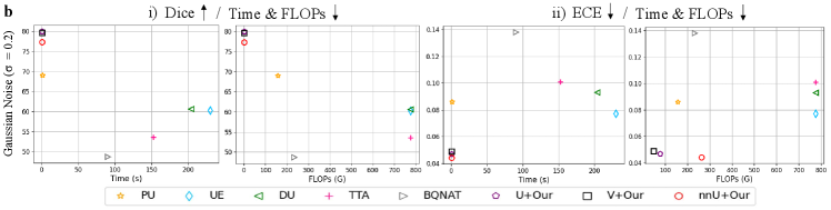
To demonstrate the effectiveness of the efficiency, we provide more insight into the computational cost performances of well-known uncertainty estimation methods (DU [18], UE [22], PU [19], TTA [46] and BQNAT [39]) on the datasets of ISIC2018, LiTS2017, and BraTS2019 with Gaussian noise by (Fig. 3 (b), Fig. 4 (b) and Fig. 5 (b)). Among the evaluated methods, UE and TTA are the least computationally efficient, yet they yield slightly better segmentation results compared to DU. BQNAT demonstrates slightly higher calculation efficiency than DU, with comparable segmentation performance to TTA. Although PU has shown improvements in both computing efficiency and segmentation results, it still requires additional sampling time for testing. After applying DEviS, fundamental deep learning models such as U-Net, Attention-UNet, V-Net, nnUNet, and Transformer segmentation methods represented by nnFormer exhibit noticeable improvements in both testing time and FLOPs compared to the previously mentioned uncertainty quantification methods. Additionally, they deliver more robust segmentation outcomes post-integration.
Moreover, we present comprehensive numerical analyses of computational efficiency, segmentation performance, and uncertainty estimation reliability. These can be found in the Tab. 1. Compared to existing uncertainty estimation methods, the integrated DEviS models manifest diminished computational efficiency while showcasing enhanced segmentation robustness. Furthermore, superior calibration outcomes are evident through metrics like ECE and UEO, signifying advancements in reliable medical image segmentation and uncertainty estimation. Specifically, in the 2D skin lesion segmentation task, models such as UE, DU, TTA, and BQNAT, which necessitate multiple predictions, exhibit slightly higher computation times, while the PU method demonstrates substantially less. The U-Net integrated with DEviS demonstrates significantly improved computation time, approximately 198, 88, and 2 times faster than the top three methods UE, BQNAT, and PU, respectively. From Tab. 1., it can be inferred that in the multi-modal 3D brain tumor segmentation task, as input data size and model complexity increase, the computation time of UE escalates, whereas TTA, BQNAT, and PU require relatively less time. In comparison to the U-Net integrated with DEviS, TTA, BQNAT, and PU methods necessitate approximately 687, 399, and 9 times more computation time, respectively. Notably, the nnFormer integrated with DEviS exhibits the highest computational efficiency, with computation times approximately 1060, 616, and 13 times faster than TTA, BQNAT, and PU methods, respectively.
Furthermore, concerning segmentation performance and uncertainty reliability, this paper evaluates segmentation efficacy using the Dice and ASSD metrics. As uncertainty lacks ground truth, the same ECE and UEO metrics as in the literature are employed to indirectly assess the reliability of uncertainty estimation. As delineated in Tab. 1., under noisy conditions, U-Net, Attention-UNet, V-Net, and nnFormer integrated with DEviS demonstrate heightened accuracy and reliability in comparison to existing uncertainty estimation methods.
4.5 DEviS empowers clinical applications.
1) Out-of-distribution detector: As shown in Fig. 2 (d), the proposed DEviS method is demonstrated to be applicable for OOD detection. It is essential that image processing systems identify any OOD samples in clinical settings. Uncertainty estimation quantifies the uncertainty of the in-distribution (ID) and OOD data to detect inputs that are far outside the training data distribution. DEviS can thus be used to alert clinicians to areas where lesions may be present in OOD data. Further, we equipped DEviS with UAF to distinguish ID and OOD samples.
We conducted OOD experiments on the Johns Hopkins OCT dataset and Duke OCT dataset with Diabetic Macular Edema (DME). As shown in Fig. 6 a, we first observed a slight improvement in results for mixed ID and OOD data after using DEviS. Then, we found significant differences in the performance of the segmentation between the with or without UAF. Additionally, there were also marked differences in the distribution of uncertainty between the ID and OOD data, especially adding the UAF module as shown in Fig. 6 b. As depicted in Fig. 6 c (i), We then employed Uniform Manifold Approximation and Projection (UMAP) to visually assess the integration of our method. In the spatial clustering results of the base network framework, we observed overlapping of ID and OOD data batches. However, after integrating DEviS, we observed improved batch-specific separation of ID and OOD data, particularly for the ID data. Furthermore, the integration of UAF with DEviS effectively eliminated the OOD, resulting in a more pronounced batch effect. Additionally, we first presented the uncertainty estimation map corresponding to UMAP in the Fig. 6 c (ii). It is evident from the map that the boundary region between different batches exhibits significantly higher uncertainty. More intuitively, the segmentation results and uncertainty maps of ID and OOD data can refer to Fig. 8 a. These results combine to show that DEviS with UAF provides a solution for filtering out abnormal areas where lesions may be present in OOD data.
2) Image quality indicator: As shown in Fig. 2 e, it demonstrates that DEviS can serve as an indicator for representing the quality of medical images. Uncertainty estimation is an intuitive and quantitative way to inform clinicians or researchers about the quality of medical images. DEviS guides image quality quantitatively through the distribution of uncertainty values and qualitatively through the degree of explicitness of the uncertainty map. Furthermore, our developed UAF module aids in the initial screening of low-quality and high-quality data. High-quality data can be directly employed in clinical practice, while low-quality data necessitates expert judgment before utilization.
In what follows, we apply DEviS with UAF to indicate the quality of data for real-world applications. The FIVES datasets are used for quality assessment experiments. We initially classified samples into three categories based on their quality labels: high quality, high & low quality, and low quality. We observed distinct performance variations among these categories (Fig. 7 a (i)). To further demonstrate its ability to indicate image quality, we delved into a combination of high and low-quality data to filter out high-quality data. Before the application of UAF, we identified 159 high-quality and 141 low-quality data samples. Upon implementing UAF, the distribution shifted, resulting in 153 high-quality and 61 low-quality data samples. This transition led to a remarkable increase in the proportion of high-quality data from 53% to 71%. Notably, the task at hand posed a greater challenge in assessing data quality compared to the detection of OOD data, as all data sources originated from the same distribution. We also found a significant performance boost with UAF in Dice and ECE metrics. (Fig. 7 a (ii)). Additionally, we investigated the distribution of uncertainty to discern differences between different qualities data (Fig. 7 b (i)). Moreover, the uncertainty distribution of high and low mixed quality with UAF was closer to the low-quality data (Fig. 7 b (ii)). The spatial clustering results of mixed-quality images were visualized using UMAP in the Fig. 7 c. Prior to incorporating our algorithm, some batch-specific separation was observed, albeit with partially overlapping regions (Fig. 7 c (i) 1st and 4th columns). However, upon integrating DEviS with UAF, a slight batch effect was observed (Fig. 7 c (i) 2nd, 3rd, 5th and 6th columns). Additionally, the UMAP visualization with uncertainty map exhibited uncertainty warnings for partially overlapping points, with noticeably high uncertainties along the edges of prediction errors (Fig. 7 c (ii) (1, 2)). Moreover, the segmentation results and uncertainty map of low-quality and high-quality images exhibited in Fig. 8 b, providing a more intuitive representation of the quality disparity. These results demonstrate that DEviS with UAF can serve as an image quality indicator to fairly value personal data in healthcare and consumer markets. This would help to remove harmful data while identifying and collecting higher-value data for diagnostic support.


DEviS proves valuable in clinical applications through its dual functionality. As an adept OOD detector, DEviS, coupled with UAF, effectively distinguishes OOD data, enhancing reliability in clinical image processing. Moreover, DEviS serves as a robust image quality indicator, offering both quantitative and qualitative assessments of medical image quality. The integration of UAF further refines this assessment, demonstrating its capability to filter high-value data and improve performance metrics. These functionalities position DEviS as a versatile tool for detecting abnormal areas in OOD data and indicating image quality, vital for diagnostic support in healthcare and other applications.


5 Discussion
Although medical image segmentation methodology is growing considerably, this has not been matched by a corresponding increase in reliability. To address this, an effective approach is to develop a model that offers computationally efficient confidence, robustness, and calibration, thereby delivering both sensitivity and interpretability for unreliable data and identifying the reliable segmentation regions for clinical specialist. In this study, we present DEviS, a novel approach for reliable medical image segmentation that offers both robust segmentation results and reliable uncertainty estimates by seamlessly integrating into existing backbone networks. To assess its reliability, we conducted experiments on three public datasets, namely ISIC2018 (2D setting) and BraTS2019 (multi-modal 3D setting), demonstrating consistent and robust performance along with computational efficiency and reliable uncertainty estimation. More importantly, we examined its potential for safe clinical applications by employing diverse datasets to validate its ability in detecting OOD data.
We analyzed differences in reliable segmentation networks between the traditional medical image segmentation methods [48, 54] and the evidential deep learning method [40]. Compared with the traditional segmentation methods [9, 48], we treat the predictions of the backbone neural network as subjective opinions instead of using the softmax layer to generate predictions with over-confident scores. As a result, our model provides pixel-wise uncertainty estimations and robust segmentation, which is essential for facilitating interpretation during disease diagnosis. Applying the evidential deep learning method [40], we develop an evidential deep segmentation framework as an easily implementable foundational model, focusing on reliable medical image segmentation. We adopt the CUP in the training to obtain more calibrated predictions. Furthermore, our research represents a significant stride towards promoting potential clinical application as we integrate an UAF strategy into the DEviS framework, emphasizing its practical implications in the medical field.
DEviS performs promisingly for segmentation of normal data, there still remains room for improvement. Flaws remain when processing high-level OOD data for clinical needs. Multi-modality MRI are directly utilized as inputs for segmentation, but we do not progress to estimate uncertainty between the different modalities. Despite this, DEviS provides a reliable shortcut to medical image segmentation for any backbone network through furnishing robust segmentation results with a visible uncertainty map for clinicians and researchers. Looking ahead, there is a need to improve the performance of robust segmentation results and uncertainty estimates under normal and abnormal data. At the same time, further exploration of multi-modal reliable medical image segmentation is also needed, as is uncertainty estimation under federated learning. All of these will lead to more reliable systems for disease diagnosis and treatment.
6 Conclusion
In conclusion, our study involves a comprehensive survey and empirical analysis of the foundational DEviS model introduced herein.This work establishes a comprehensive framework for achieving reliable medical image segmentation, enabling the identification of dependable segmentation regions and ultimately fostering trust between healthcare professionals and deep learning models. Our framework excels in generating accurate and well-calibrated segmentation results while ensuring high computational efficiency in uncertainty estimation. We first efficiently model uncertainty for different classes of segmentation results by leveraging subjective logic theory. Moreover, we developed the CUP to generate more calibrated confidence and maintain the segmentation performance of the base network. Besides, the proposed UAF strategy offers a viable pathway to ensure the necessary assurance for its effective integration into subsequent clinical task, such as OOD data detection. We evaluated the reliability of DEviS with different public datasets consisting of different data modalities and different target structures. We demonstrate here that DEviS with UAF achieves a superior performance with potential ease of interpretation in medical image segmentation for reliable diagnostic support and quantitative assessments of medical data. We are confident that our work can potentially benefit researchers in the reliable medical domain.
References
- [1] C. F. Baumgartner, K. C. Tezcan, K. Chaitanya, A. M. Hötker, U. J. Muehlematter, K. Schawkat, A. S. Becker, O. Donati, and E. Konukoglu. Phiseg: Capturing uncertainty in medical image segmentation. In International Conference on Medical Image Computing and Computer-Assisted Intervention, pages 119–127. Springer, 2019.
- [2] P. Bilic, P. Christ, H. B. Li, E. Vorontsov, A. Ben-Cohen, G. Kaissis, A. Szeskin, C. Jacobs, G. E. H. Mamani, G. Chartrand, et al. The liver tumor segmentation benchmark (lits). Medical Image Analysis, 84:102680, 2023.
- [3] Ö. Çiçek, A. Abdulkadir, S. S. Lienkamp, T. Brox, and O. Ronneberger. 3d u-net: Learning dense volumetric segmentation from sparse annotation. In Medical Image Computing and Computer-Assisted Intervention – MICCAI 2016, pages 424–432, Cham, 2016. Springer International Publishing.
- [4] A. P. Dempster. A Generalization of Bayesian Inference, chapter 4, pages 73–104. Springer Berlin Heidelberg, Berlin, Heidelberg, 2008.
- [5] R. Deng, C. Cui, L. W. Remedios, S. Bao, R. M. Womick, S. Chiron, J. Li, J. T. Roland, K. S. Lau, Q. Liu, et al. Cross-scale multi-instance learning for pathological image diagnosis. Medical Image Analysis, page 103124, 2024.
- [6] A. Dosovitskiy, L. Beyer, A. Kolesnikov, D. Weissenborn, X. Zhai, T. Unterthiner, M. Dehghani, M. Minderer, G. Heigold, S. Gelly, et al. An image is worth 16x16 words: Transformers for image recognition at scale. arXiv preprint arXiv:2010.11929, 2020.
- [7] T. Falk, D. Mai, R. Bensch, Ö. Çiçek, A. Abdulkadir, Y. Marrakchi, A. Böhm, J. Deubner, Z. Jäckel, K. Seiwald, et al. U-net: deep learning for cell counting, detection, and morphometry. Nature methods, 16(1):67–70, 2019.
- [8] Y. Gal and Z. Ghahramani. Dropout as a bayesian approximation: Representing model uncertainty in deep learning. In international conference on machine learning, pages 1050–1059. PMLR, 2016.
- [9] R. Gu, G. Wang, T. Song, R. Huang, M. Aertsen, J. Deprest, S. Ourselin, T. Vercauteren, and S. Zhang. Ca-net: Comprehensive attention convolutional neural networks for explainable medical image segmentation. IEEE Transactions on Medical Imaging, 40(2):699–711, 2020.
- [10] C. Guo, G. Pleiss, Y. Sun, and K. Q. Weinberger. On calibration of modern neural networks. In International Conference on Machine Learning, pages 1321–1330. PMLR, 2017.
- [11] C. Guo, G. Pleiss, Y. Sun, and K. Q. Weinberger. On calibration of modern neural networks. In International conference on machine learning, pages 1321–1330. PMLR, 2017.
- [12] Z. Han, C. Zhang, H. Fu, and J. T. Zhou. Trusted multi-view classification with dynamic evidential fusion. IEEE transactions on pattern analysis and machine intelligence, 45(2):2551–2566, 2022.
- [13] K. He, X. Chen, S. Xie, Y. Li, P. Dollár, and R. Girshick. Masked autoencoders are scalable vision learners. In Proceedings of the IEEE/CVF conference on computer vision and pattern recognition, pages 16000–16009, 2022.
- [14] L. Huang, S. Ruan, P. Decazes, and T. Denoeux. Lymphoma segmentation from 3d pet-ct images using a deep evidential network. International Journal of Approximate Reasoning, 149:39–60, 2022.
- [15] F. Isensee, P. F. Jaeger, S. A. Kohl, J. Petersen, and K. H. Maier-Hein. nnu-net: a self-configuring method for deep learning-based biomedical image segmentation. Nature methods, 18(2):203–211, 2021.
- [16] A. Jøsang. Subjective logic: A Formalism for Reasoning Under Uncertainty. Springer, Cham, 2016.
- [17] A. Jungo and M. Reyes. Assessing reliability and challenges of uncertainty estimations for medical image segmentation. In International Conference on Medical Image Computing and Computer-Assisted Intervention, pages 48–56. Springer, 2019.
- [18] A. Kendall and Y. Gal. What uncertainties do we need in bayesian deep learning for computer vision? Advances in neural information processing systems, 30, 2017.
- [19] S. Kohl, B. Romera-Paredes, C. Meyer, J. De Fauw, J. R. Ledsam, K. Maier-Hein, S. Eslami, D. Jimenez Rezende, and O. Ronneberger. A probabilistic u-net for segmentation of ambiguous images. Advances in Neural Information Processing Systems, 31, 2018.
- [20] R. Krishnan and O. Tickoo. Improving model calibration with accuracy versus uncertainty optimization. Advances in Neural Information Processing Systems, 33:18237–18248, 2020.
- [21] S. Lacoste-Julien, F. Huszar, and Z. Ghahramani. Approximate inference for the loss-calibrated bayesian. In International Conference on Artificial Intelligence and Statistics, pages 416–424, 2011.
- [22] B. Lakshminarayanan, A. Pritzel, and C. Blundell. Simple and scalable predictive uncertainty estimation using deep ensembles. Advances in Neural Information Processing Systems, 30, 2017.
- [23] X. Li, H. Chen, X. Qi, Q. Dou, C.-W. Fu, and P.-A. Heng. H-denseunet: Hybrid densely connected unet for liver and tumor segmentation from ct volumes. IEEE Transactions on Medical Imaging, 37(12):2663–2674, 2018.
- [24] S. Liang, Y. Li, and R. Srikant. Enhancing the reliability of out-of-distribution image detection in neural networks. arXiv preprint arXiv:1706.02690, 2017.
- [25] W. Liang, G. A. Tadesse, D. Ho, L. Fei-Fei, M. Zaharia, C. Zhang, and J. Zou. Advances, challenges and opportunities in creating data for trustworthy ai. Nature Machine Intelligence, 4(8):669–677, 2022.
- [26] Y. Liu, H. Wang, Z. Chen, K. Huangliang, and H. Zhang. Transunet+: Redesigning the skip connection to enhance features in medical image segmentation. Knowledge-Based Systems, 256:109859, 2022.
- [27] J. Long, E. Shelhamer, and T. Darrell. Fully convolutional networks for semantic segmentation. In Proceedings of the IEEE conference on computer vision and pattern recognition, pages 3431–3440, 2015.
- [28] A. Mehrtash, W. M. Wells, C. M. Tempany, P. Abolmaesumi, and T. Kapur. Confidence calibration and predictive uncertainty estimation for deep medical image segmentation. IEEE Transactions on Medical Imaging, 39(12):3868–3878, 2020.
- [29] R. Mehta, T. Christinck, T. Nair, et al. Propagating uncertainty across cascaded medical imaging tasks for improved deep learning inference. IEEE Transactions on Medical Imaging, 41(2):360–373, 2021.
- [30] B. H. Menze, A. Jakab, S. Bauer, J. Kalpathy-Cramer, et al. The multimodal brain tumor image segmentation benchmark (brats). IEEE Transactions on Medical Imaging, 34(10):1993–2024, 2015.
- [31] F. Milletari, N. Navab, and S.-A. Ahmadi. V-net: Fully convolutional neural networks for volumetric medical image segmentation. In 2016 Fourth International Conference on 3D Vision (3DV), pages 565–571, 2016.
- [32] J. Mukhoti and Y. Gal. Evaluating bayesian deep learning methods for semantic segmentation. arXiv preprint arXiv:1811.12709, 2018.
- [33] J. Mukhoti, A. Kirsch, J. van Amersfoort, P. H. Torr, and Y. Gal. Deep deterministic uncertainty: A new simple baseline. In Proceedings of the IEEE/CVF Conference on Computer Vision and Pattern Recognition, pages 24384–24394, 2023.
- [34] J. Mukhoti, J. van Amersfoort, P. H. Torr, and Y. Gal. Deep deterministic uncertainty for semantic segmentation. In International Conference on Machine Learning Workshop on Uncertainty and Robustness in Deep Learning, pages 1–5, 2021.
- [35] T. Nair, D. Precup, D. L. Arnold, and T. Arbel. Exploring uncertainty measures in deep networks for multiple sclerosis lesion detection and segmentation. Medical image analysis, 59:101557, 2020.
- [36] O. Oktay, J. Schlemper, L. L. Folgoc, M. Lee, M. Heinrich, K. Misawa, K. Mori, S. McDonagh, N. Y. Hammerla, B. Kainz, et al. Attention u-net: Learning where to look for the pancreas. In Medical Imaging with Deep Learning, pages 1–10, 2018.
- [37] V. Oreiller, V. Andrearczyk, M. Jreige, S. Boughdad, H. Elhalawani, J. Castelli, M. Vallières, S. Zhu, J. Xie, Y. Peng, et al. Head and neck tumor segmentation in pet/ct: the hecktor challenge. Medical image analysis, 77:102336, 2022.
- [38] Y. Ovadia, E. Fertig, J. Ren, Z. Nado, D. Sculley, S. Nowozin, J. Dillon, B. Lakshminarayanan, and J. Snoek. Can you trust your model’s uncertainty? evaluating predictive uncertainty under dataset shift. Advances in neural information processing systems, 32, 2019.
- [39] A. G. Roy, S. Conjeti, N. Navab, C. Wachinger, A. D. N. Initiative, et al. Bayesian quicknat: Model uncertainty in deep whole-brain segmentation for structure-wise quality control. NeuroImage, 195:11–22, 2019.
- [40] M. Sensoy, L. Kaplan, and M. Kandemir. Evidential deep learning to quantify classification uncertainty. In Proceedings of the 32nd International Conference on Neural Information Processing Systems, pages 3183–3193, 2018.
- [41] N. M. Temme. Special functions: An introduction to the classical functions of mathematical physics. John Wiley & Sons, 1996.
- [42] P. Tschandl, C. Rosendahl, and H. Kittler. The ham10000 dataset, a large collection of multi-source dermatoscopic images of common pigmented skin lesions. Scientific data, 5(1):1–9, 2018.
- [43] J. Van Amersfoort, L. Smith, Y. W. Teh, and Y. Gal. Uncertainty estimation using a single deep deterministic neural network. In International Conference on Machine Learning, pages 9690–9700. PMLR, 2020.
- [44] A. Vaswani, N. Shazeer, N. Parmar, J. Uszkoreit, L. Jones, A. N. Gomez, Ł. Kaiser, and I. Polosukhin. Attention is all you need. Advances in neural information processing systems, 30, 2017.
- [45] G. Wang, W. Li, M. Aertsen, J. Deprest, S. Ourselin, and T. Vercauteren. Aleatoric uncertainty estimation with test-time augmentation for medical image segmentation with convolutional neural networks. Neurocomputing, 338:34–45, 2019.
- [46] G. Wang, W. Li, S. Ourselin, and T. Vercauteren. Automatic brain tumor segmentation using convolutional neural networks with test-time augmentation. In International MICCAI Brainlesion Workshop, pages 61–72. Springer, 2018.
- [47] M. Wang, T. Lin, L. Wang, A. Lin, K. Zou, X. Xu, Y. Zhou, Y. Peng, Q. Meng, Y. Qian, et al. Uncertainty-inspired open set learning for retinal anomaly identification. Nature Communications, 14(1):6757, 2023.
- [48] W. Wang, C. Chen, M. Ding, H. Yu, S. Zha, and J. Li. Transbts: Multimodal brain tumor segmentation using transformer. In Medical Image Computing and Computer Assisted Intervention – MICCAI 2021, pages 109–119, 2021.
- [49] X. Wang, S. Yang, J. Zhang, M. Wang, J. Zhang, W. Yang, J. Huang, and X. Han. Transformer-based unsupervised contrastive learning for histopathological image classification. Medical image analysis, 81:102559, 2022.
- [50] J. Wu, C. Li, M. Gensheimer, et al. Radiological tumour classification across imaging modality and histology. Nature Machine Intelligence, 3(9):787–798, 2021.
- [51] R. Zeleznik, B. Foldyna, P. Eslami, et al. Deep convolutional neural networks to predict cardiovascular risk from computed tomography. Nature communications, 12(1):1–9, 2021.
- [52] H. Zhang, L. Chen, X. Gu, M. Zhang, Y. Qin, F. Yao, Z. Wang, Y. Gu, and G.-Z. Yang. Trustworthy learning with (un) sure annotation for lung nodule diagnosis with ct. Medical Image Analysis, 83:102627, 2023.
- [53] H. Zhang, X. Hong, S. Zhou, and Q. Wang. Infrared image segmentation for photovoltaic panels based on res-unet. In Chinese Conference on Pattern Recognition and Computer Vision (PRCV), pages 611–622. Springer, 2019.
- [54] H.-Y. Zhou, J. Guo, Y. Zhang, X. Han, L. Yu, L. Wang, and Y. Yu. nnformer: Volumetric medical image segmentation via a 3d transformer. IEEE Transactions on Image Processing, 2023.
- [55] Z. Zhou, M. M. R. Siddiquee, N. Tajbakhsh, and J. Liang. Unet++: Redesigning skip connections to exploit multiscale features in image segmentation. IEEE Transactions on Medical Imaging, 39(6):1856–1867, 2020.
- [56] K. Zou, Z. Chen, X. Yuan, X. Shen, M. Wang, and H. Fu. A review of uncertainty estimation and its application in medical imaging. Meta-Radiology, page 100003, 2023.
- [57] K. Zou, X. Yuan, X. Shen, M. Wang, and H. Fu. Tbrats: Trusted brain tumor segmentation. In International Conference on Medical Image Computing and Computer-Assisted Intervention, pages 503–513. Springer, 2022.
Appendix A Gradient Analysis for
According to Eq. 17, the loss function can be written as:
| (S1) |
where . Then the gradient of the above formula can be computed as:
| (S2) |
From the above formula, we can get the local optimum by . Since is the function, we employ the approximation [41] to analyze the role of uncertainty. Substituting into Eq. S2, the second term can be approximated as . In addition, corresponding to denotes the distances between the sample and ground truth. Therefore, the gradient of above formula can be rewritten as:
| (S3) |
For the first term , the optimization process becomes more difficult once the becomes larger. So, the parameter plays a crucial role in determining the proximity of the sample to the ground truth, thereby exerting a significant influence on the optimization process. In other words, it calculates the loss of predictions and facilitates the smooth local optima. For the second term , is approximated to . Therefore, if the uncertainty in the second term increases, higher gradients will be generated for the optimization. In other words, the second term captures the uncertainty, that is, the uncertainty will become larger when the hard sample appears.
Appendix B Calibrated uncertainty penalty
The calibrated uncertainty attempts involve additional steps in the standard DEviS loss formulation, which can be represented as follows:
| (S4) |
During the training, we train the model with a higher DEviS loss, allowing the model to learn the uncertainty threshold required for applying the CUP loss. The proposed CUP loss acts as a utility-dependent penalty term within the loss-calibrated inference framework. The CUP loss serves as a utility function that guides optimal predictions to achieve well-calibrated uncertainties, ensuring more accurate and reliable predictions. In theory, the CUP loss will be equal to 0 only when the model’s uncertainty is perfectly calibrated (maximizing the utility function, CUP = 1). As described in equations 9 and 10, the aims to maximize the utility function CUP, indirectly adjusting the uncertainty values based on the predictive accuracy. It can be denoted as:
| (S5) |
Consequently, the increases for inaccurate and uncertain samples during early training. As training progresses, the is further increased to prioritize accurate and deterministic samples. In this way, we can simplify the above equation to Eq. 20.
More intuitively, we show the four possible toy examples of DEviS output in Fig. S1. The first is a sloped and sharp Dirichlet simplex specification model that makes accurate and certain (A&C) predictions (Fig. S1 (a)), as opposed to an unsloped and flat Dirichlet simplex specification model that makes inaccurate and uncertain (I&U) (Fig. S1 (d)). In addition, the model may also produce a sloped and flat Dirichlet simplex, that is, accurate and uncertain (A&U) predictions (Fig. S1 (b)), and an unsloped and sharp Dirichlet simplex, that is, inaccurate and certain (I&C) predictions (Fig. S1 (c)). Following the same goal as [20], we encourage DEviS to learn a skewed and sharp Dirichlet simplex in the early training (Fig. S1 (a)). In addition, we encourage DEviS to provide an unsloped and flat Dirichlet simplex for incorrect predictions in the late training (Fig. S1 (d)). This stems from the fact that if a pixel is assigned a high uncertainty, the pixel is more likely to be incorrect, thereby identifying an unknown pixel. To this end, we design the uncertainty calibration loss function as Eq. 20, which regularizes DEviS training by minimizing the expectations of A&C and I&U samples (Fig. S1 (a) and Fig. S1 (d)) such that the other cases (A&U in Fig. S1 (b) and I&C in Fig. S1 (c)) can be discouraged. The first term in Eq. 20 is designed to give low uncertainty when the model predictions are accurate, while the second term in Eq. 20 attempts to give high uncertainty when the model predictions are inaccurate. At the same time, we adopt the annealing weighting factor to achieve different penalties. In the early training stage, inaccurate predictions dominate, so the second term (I&C loss) should be penalized more, while in late training, accurate predictions dominate, so the first term (A&U loss) should be penalized more punishment.

Appendix C More visual comparisons

