Towards Open-Set Text Recognition via Label-to-Prototype Learning
Abstract
Scene text recognition is a popular topic and extensively used in the industry. Although many methods have achieved satisfactory performance for the close-set text recognition challenges, these methods lose feasibility in open-set scenarios, where collecting data or retraining models for novel characters could yield a high cost. For example, annotating samples for foreign languages can be expensive, whereas retraining the model each time when a “novel” character is discovered from historical documents costs both time and resources. In this paper, we introduce and formulate a new open-set text recognition task which demands the capability to spot and recognize novel characters without retraining. A label-to-prototype learning framework is also proposed as a baseline for the proposed task. Specifically, the framework introduces a generalizable label-to-prototype mapping function to build prototypes (class centers) for both seen and unseen classes. An open-set predictor is then utilized to recognize or reject samples according to the prototypes. The implementation of rejection capability over out-of-set characters allows automatic spotting of unknown characters in the incoming data stream. Extensive experiments show that our method achieves promising performance on a variety of zero-shot, close-set, and open-set text recognition datasets.
1 Introduction
Text recognition is gaining popularity among both researchers and industry fellows due to its vast applications. Currently, many scene text recognition methods [3, 31, 38] have achieved promising performance on the close-set text recognition benchmarks. However, most existing methods always fail to handle novel (unseen) characters that do not appear in the training set. Specifically, these methods model the prototypes (centers) of classes as latent weights of a linear classifier. However, adding weights for novel characters will be difficult without retraining the model. This caveat makes conventional methods unfeasible as collecting and annotating data can be very time-consuming and expensive. For example, the annotation of minority languages and ancient documents could take a long time period and yield high personnel costs. Also, novel characters may be continuously discovered from the incoming data stream, especially when processing historical documents or internet oriented images. In such cases, retraining the model each time a novel character is found would yield considerable time and resource costs.
In the literature, a few text recognition methods are capable to handle novel characters. These methods can be divided into two different schemes. One category [5, 37, 49] exploits the radical composition of each character, consequentially limiting most of them to the Chinese language. Another category is based on weight imprinting [24], which generates prototypes with corresponding glyphs [1, 47, 33]. Despite showing no language-specific limitation, many do not scale well on large label sets due to the training cost of the imprinting module. For both categories, despite a few methods possessing text-line recognition capability [49, 13, 47], very few demonstrate competitive performance on standard close-set benchmarks [2], limiting their feasibility in practice.
Furthermore, the aforementioned zero-shot text recognition methods are not capable to reject “out-of-set” samples like Open Set Recognition (OSR) methods [10, 9]. The rejection capability can help the users to quickly spot newly emerging characters in the incoming data stream, whereas the recognition capability enables a quick adaption without retraining the model. Combining these two capabilities yields a human-in-the-loop recognition system capable to evolve with the input data, which we formulate as the open-set text recognition task. Here, we propose a label-to-prototype learning framework to efficiently address this new task in a language-agnostic manner, while preserving competitive performance on close-set benchmarks. To dynamically build prototypes for both seen and unseen (novel) characters, a label-to-prototype module is proposed to map each character to its corresponding prototypes (classifier weights) by encoding glyphs of all its cases. The module augments the conventional text recognition framework [2] as an extra stage. The open-set predictor is then introduced to categorize or reject character features at each-time stamp according to its similarities with the dynamically generated prototypes, replacing the linear classifier in the Pred. stage [2]. Moreover, we propose a lightweight topology preserving rectification module to handle skewed samples. The module applies a mesh-grid transformation to intermediate feature maps, with parameter estimation fused with the backbone avoiding dedicated rectification networks like [2, 20, 43]. A variety of quantitative and qualitative experiments show that our proposed framework achieves promising performance on all open-set, zero-shot, and close-set text recognition datasets.
In summary, our main contributions are:
-
1.
Formulating the open-set text recognition task that demands further capabilities to spot novel characters and adapt to recognize them without retraining the model.
-
2.
Proposing a label-to-prototype learning framework capable to address novel characters while keeping reasonable speed and competitive performance on conventional benchmarks.
-
3.
Proposing a topology-preserving transformation technique for text recognition by performing fast fine-grained rectification alongside the feature extraction.
2 Open-Set Text Recognition
2.1 Task Definition

Generally speaking, the open-set text recognition task (OSTR, illustrated in Fig. 1) extracts text from images that potentially contain novel characters unseen in the training set. Specifically, a character is considered “novel” if , where is the set of all characters that appear in the training samples. Likewise, characters of the testing set form the testing character set . can be disjointly divided into for “in-set” characters with corresponding side-information provided during evaluation, and for “out-of-set” characters without side-information. Here, side-information refers to label information that uniquely defines a character, e.g., glyphs [47], component composition [4, 5], or other equivalent information. The task requires recognizing characters in w.r.t. the provided side-information and reject the characters from by predicting them as the “unknown” label ‘[-]’.
Note in applications, refers to all characters in the entire data stream. Hence in many cases users have no prior knowledge of novel characters at the beginning. However, when novel characters are spotted by inspecting rejected samples, the user can move them to for future recognition, by providing their side-information to the model. Vice versa, the user may move an obsolete character from to by removing its side-information. Hence, can be volatile as a result of users adding or removing characters. For addressing convenience, we accordingly divide characters to 4 categories as shown in Figure 1: “Seen In-set Character (SIC)”, “Seen Out-of-set Character (SOC)”, “Novel In-set Character (NIC)”, and the “Novel Out-of-set Character (NOC)”. The first term indicates whether the character is “seen” or “novel” to training samples, and the second tells whether it is in with its side-information provided for evaluation.
Metric-wise, two popular metrics in the text recognition community are used to evaluate the recognition performance. One is the line accuracy(LA) 333The line accuracy is also known as word accuracy (WA), same to 1-WER (Word Error Rate). [2], defined as,
| (1) |
where is the size of the dataset, and correspondingly indicate the label and the prediction of the sample. Another is the character accuracy (CA) 444The character accuracy is also known as accuracy rate (AR), same to 1-NED (normalized edit distance). [7],
| (2) |
The capability to reject characters in is measured with word-level recall (), precision (), and F-measure ().
| (3) |
Here, is an indicator function that returns whether the string contains “out-of-set” characters (SOC and NOC). Since word samples containing out-of-set characters (predicted as “unknown”) require human inspection whether “in-set” characters appear or not, we use word-level measurements for simplicity. Specifically, the recall describes the likelihood for the system to reject a sample containing “out-of-set” characters and alert the user to adjust . The precision measures the ratio of fake positive warnings needing manual dismissal. Finally, the F-measure is given as an overall metric of recall and precision,
| (4) |
2.2 Dataset
In this work, we construct an open-set text recognition dataset with a collection of existing openly available datasets. Here, we choose Chinese scene text images for training while Japanese scene text images for evaluation, due to the abundant amount of samples that can be found in these two languages. The list of upstream datasets and the processing scripts are also released alongside our codes555https://github.com/lancercat/OSOCR. Specifically, the training set contains Chinese and Latin samples collected from ART [7], RCTW [32], LSVT [34], CTW [45], and the Latin-Chinese subset of the MLT dataset 666Crops with language annotated as Latin and Chinese.. The character-set contains Tier-1 simplified Chinese characters, English letters(‘A’-‘z’), and digits (‘0’-‘9’). Samples with characters not covered by are excluded from the training set. The testing dataset contains Japanese samples drawn from the MLT dataset. The character-set contains all characters that appear in this subset.
The evaluation is performed under five setups using different splits over . The first setup is closer to the generalized zero-shot learning tasks (GZSL) where all characters go to . The second splits all novel characters to to match the open-set recognition (OSR) setup. The third introduces SOC to the second setup. The fourth split the Hiragana and Katakana into , imitating the GOSR setup. Finally, the fifth introduces SOC to of task four, implementing the full OSTR task. To simplify the task and focus on the open-set problem, we remove all vertical texts in the training and testing sets. The testing set contains a total of text lines in the testing set. Note that because the character-sets of Japanese and Chinese overlap, the conventional close-set methods do not yield a zero accuracy.
3 Related Works
3.1 Relations with Other Tasks
The open-set text recognition (OSTR) task can be regarded as a combination of the open-set recognition task(OSR) [26, 41, 42] and the GZSL task [23]. Specifically, the OSTR requires recognizing both seen and novel characters in with side-information like GZSL tasks [23]. Furthermore, the OSTR requires the rejection capability on samples from classes not covered by , seen or unseen. Despite the subjects for rejection being slightly different, Both OSTR and OSR imply closed decision boundaries for each class to recognize. In summary, compared to the GZSL tasks, the OSTR task further adds the requirement on rejection capability, which enables actively spotting samples from “out-of-set” classes (not in ) in applications. Compared with the OSR task, besides the capability to spot samples from novel classes from the data stream, the OSTR introduced the capability to recognize samples from novel classes once the corresponding side-information provided, allowing fast and incremental model adaption without retraining the model. Noteworthy, the recognition capability of novel classes with closed decision boundaries implies that the samples of each novel class shall gather closely to its class center(s). Since this “gather” property is not affected by whether the side-information is known to the model, “cognition” on “unknown unknown classes” [10] is implemented in the OSTR task. Hence, the OSTR task can be considered as a variant of the generalized open-set text recognition as well.
The proposed task is also related to several existing text recognition tasks as summarized in Table 1. Compared to the close-set text recognition task solely focusing on the SIC, the OSTR task relaxes the assumption by introducing novel labels which do not appear in the training samples. On the other hand, compared to the zero-shot character recognition task [4, 37] which can also be regarded as a special case of OSTR when , , and all samples have a constant length of . Furthermore, compared to both tasks, the OSTR task introduces the rejection of out-of-set characters, allowing two folds of capability. First, the rejection capability would allow the user to get a notification when novel characters appear in the data stream. Second, it allows the user to optionally skip recognition of rare characters to speed up, while keeping track of the rejected samples, which may include the skipped characters, for later checking.
3.2 Close-Set Text Recognition
Most conventional text recognition methods can fit into the four-stage framework [2], i.e., transformation (Trans.), feature extraction (Feat.), sequence modeling (Seq.), and prediction (Pred.). The Trans. stage rectifies the input image, which can be omitted in some methods [38, 29]. In [2] and [30], a spatial transformer network is used for automatic rectification, other methods [43, 20] construct heavier neural networks and implement more complex transforms. The Feat. stage generally uses a convolutional network to extract visual features from the rectified images, e.g., ResNet [12], RCNN [15], and VGG [22]. The Seq. stage captures the contextual information of the whole sequence, by using LSTM layers [6, 29, 38], transformers [16], or simply nothing [3]. The Pred. Stage decodes the feature map into predictions. Typical implementations can be divided into two categories according to whether the segmentation is explicitly supervised. Specifically, implicitly supervised segmentation include RNN-Attention decoders [17], CTC [29], and decoupled attention decoders [38]. On the other hand, explicit segmentation methods generally implement this stage with semantic segmentation heads, e.g., TextSpotter [36] and CA-FCN [18]. In this stage, a linear classifier is adopted by most implementations to decode the segmented feature at each timestamp into character prediction. The linear classifier, in a more general way to put it, can be treated as a “character classifier” as it decodes its input into “characters”. 777Depending on the methods, the “characters” may include special tokens, e.g., in CTC based methods and “EOS” for RNN-Attention based methods.
Due to the latent nature of weights in the linear predictor, constructing corresponding weights for a novel label can be difficult without retraining. Here, our proposed framework introduces a label-to-prototype module as an extra stage to construct prototypes for both novel and seen characters. An open-set prediction module is also proposed to replace the linear classifier used in the Pred. stage offering rejection capability of “out-of-set” characters including NOC and SOC characters.
3.3 Zero-Shot Text Recognition
Most current zero-shot text recognition methods focus on Chinese Character recognition due to its challenging large character-set. However, many methods [37, 4, 13, 5] require detailed annotations on the radical composition of each character (mainly the radical composition tree or stroke sequence of a character). Such knowledge is mostly used at the decoder-side and implemented as an RNN which is hard to parallelize [13]. Some recent methods are seen to use it on the encoder side [1, 4, 13], which can avoid the RNN radical decoding process during evaluation. A few radical-based methods like [13, 49] are capable to perform Chinese text line recognition tasks on private datasets. However, mapping labels to corresponding component sequences requires strong domain knowledge and the annotating process is also a tedious job. Furthermore, text components are mainly specific to Chinese characters, which practically limits the feasibility in multi-language scenarios. Recently, Zhang et al. [47] proposed a visual-matching-based method that can handle novel characters in text lines without language limitations. However, this method would yield a significant computation burden during training, for encoding a large “glyph-line image” caused by the large charset. Also, this method shows very limited performance on conventional close-set benchmarks, which renders it less feasible for real-world applications.
Our proposed method only takes templates from the Noto fonts and does not need any domain knowledge of the specific language. Furthermore, the rejection capability, vital to active novel characters spotting, is missing for most methods. Hence, these methods cannot be considered full open-set recognition methods. Currently, zero-shot text recognition methods are mostly benchmarked on property datasets [13, 49], or datasets with a limited number of distinctive classes [47]. Thus, we provide an openly accessible open-set benchmark dataset in this work.

4 Proposed Framework
4.1 Framework Overview
In this work, we propose a label-to-prototype learning framework (Fig. 2) as a baseline of the proposed OSTR task, while retaining competitive performance on standard close-set [2] and zero-shot Chinese character [4] benchmarks. The proposed framework is composed of four main parts, namely the Recognition Backbone (Sec. 4.2), the Label-to-prototype Module (Sec. 4.3), the Open-set-Predictor (Sec. 4.4), and the Label Sampler (Sec. 4.5). Specifically, the Recognition Backbone locates, sorts, and extracts visual features of each character in the input sample. Most conventional text recognition methods can be used for this part after removing the linear classifier.888Methods with a recurrent decoder [17, 27] need an extra change on the “hidden state” to remove the dependency on history predictions. The label-to-prototype learning module provides a tractable mapping from side information of a character label to its corresponding prototypes , each defining the center of a corresponding “case” of the character. E.g., ‘a’ returns two prototypes, one for uppercase ‘A’ and another for lowercase ‘a’. The Open-set Predictor is then used to categorize or reject each input character features according to the decision boundaries, defined with corresponding prototypes and the globally shared radius . Finally, the Label Sampler is proposed for the training phase to produce out-of-set samples and reduce the training burden of the label-to-prototype learning module by sampling a reasonable portion of labels from all training characters at each iteration.
4.2 Topology-Preserving Transformation Network
For the Recognition Backbone, we implement a Topology-Preserving Transformation Network (TPTNet) adapted from the Decoupled Attention Network (DAN). [38] Like DAN, the TPTNet first extracts visual feature with a ResNet backbone, then a Concurrent Attention Module (CAM) is adopted to sample the character feature sequence from . The RNN used to model the contextual information is removed for speed-performance trade-off.

In this work, a fused-in feature-level mesh grid rectification is proposed to alleviate the common vulnerability of perspective transformations and various irregular distortions. The fused block (Fig. 3) takes a feature map as input, and produces a processed and rectified feature map as output. Specifically, the feature map is first processed into a local feature map with a convolutional block,
| (5) |
Next, we estimate the feature density on the direction and on the direction with corresponding functions and ,
| (6) |
where indicates convolution layers and is a constant number controlling the extent of rectification that the module can perform. The densities and are then integrated and normalized into the coordination mapping ,
| (7) |
Specifically, maps the coordination from the rectified feature map to the source feature map , and the mesh-grid transformation is implemented by sampling into according to with a linear sampler. As the density is always greater than zero, the integration is able to preserve the input topology, i.e, lines without intersection will not intersect after the transformation and vice-versa. The gradients of coordinates are computed similarly to the deformable convolution network in [8]. The estimation of transformation parameters shares most computation with the feature extraction, avoiding costly dedicated rectification networks in conventional approaches [20, 43].
4.3 Label-to-Prototype Learning Module
The key point of open-set text recognition is to construct a tractable mapping from the label space to the prototype space , which can be applied to both seen and novel characters. Note could potentially be a one-to-many mapping as a character may have multiple cases. In this work, we propose the label-to-prototype learning module decomposing into two mappings, namely and , by introducing the intermediate template space containing glyphs drawn from the Noto-font. 999The Noto fonts for most languages are available at https://noto-website-2.storage.googleapis.com/pkgs/Noto-unhinted.zip.
Here, maps each character in the character set to the glyphs of all its cases. “Case” here refers to different forms of a character, e.g., upper-case and lower-case, simplified Chinese and traditional Chinese, Hiragana and Katakana, and different contextual shapes as in Arabic. As the Noto-font covers most characters in many languages with a uniform style, is highly likely to generalize to novel characters not appearing in the training set. Also, requires little domain knowledge of the specific languages, e.g. , part information and composition information for each character.
is the mapping from the template space to the prototype space. The mapping is implemented with the ProtoCNN module, which includes a ResNet18 network, a normalization layer, and a trainable latent prototype for the end-of-speech “character” (‘[s]’). Prototypes of normal characters are generated by encoding and normalizing the corresponding glyphs with the ResNet,
| (8) |
The normalization is conducted to alleviate the effect of the potential bias of character frequency between the training set and the testing set. For to be generalizable to novel classes, the templates of seen characters need to fill the template space densely enough, which requires the framework to be trained on languages with large character-sets. As the normalized prototypes can be cached before evaluation and updated incrementally on character-set change, the evaluation-time overhead is negligible.
4.4 Open-Set Predictor
In this work, an open-set predictor is proposed to replace the linear classifiers used in conventional text recognition methods [2]. Like the classifiers in the weight imprinting methods [24], the open-set predictor performs classification for characters in by comparing the generated prototypes to visual features. The module further adopts closed decision boundaries [9, 48] to achieve rejection on “out-of-set” characters (in ) not similar to any provided prototypes.
Specifically, the open-set predictor first computes the “case-specific” similarity scores via the scaled product of the visual feature and the normalized prototype matrix ,
| (9) |
Here, the similarity score of the feature at timestamp and the prototype can be written as,
| (10) |
Since is a constant number given a certain timestamp , can be interpreted as the scaled cosine similarities between all prototypes in and the visual feature . Thus, is detonated as the similarity score. Due to the exponential operator in the Softmax function, controls how much the predicted probability would be close to one-hot. Hence, is interpreted as the confidence of timestamp , and interprets as the overall model confidence. Also, since can be interpreted as the overall “preference” of prototype , the prototypes are normalized in the label-to-prototype module to alleviate potential frequency-related bias.
The module then applies max reduction on case-wise similarity , producing the label-wise classification scores , i.e.,
| (11) |
where is the label function that reduces all prototypes to labels, and the extra one comes from the “end-of-speech” token. Specifically, returns the character which has the template as one of its cases. Combining this strategy with the mapping operation in the label-to-prototype module allows us to train the framework with case agnostic annotations, without explicitly aligning cases with drastic appearance differences to the same region on the prototype space , e.g., ’A’ and ’a’. The module rejects samples not similar to any provided prototypes by predicting them into the “out-of-set” label ‘[-]’. The “out-of-set” label is not associated with a dedicated prototype as it covers many characters that do not share common visual traits. Instead, the module uses a trainable score attached to as the similarity score for the “out-of-set” label at each timestamp , yielding the final score vector ,
| (12) |
During training, the classification loss pushes above other scores on “out-of-set” characters, for “in-set” characters, is pushed below the score of correct classes. During evaluation, “out-of-set” characters would yield similarities less than to any prototypes due to the shape difference, yielding a rejection. Hence, can also be interpreted as the radius of the decision boundary [9], or a similarity threshold.

4.5 Optimization
In this work, a label sampler (illustrated in Fig 4) is proposed to introduce “out-of-set” samples and control complexity during training. For each batch of training data, the sampler constructs a character-set , composed of three disjoint subsets: the “positive” characters , the “negative” characters , and the special tokens101010The end-of-speech label ‘[s]’ and the unknown label ‘’.
Here, the module first collects all characters that appear in the batch, denoted as . Then, it samples a fraction of the as the “positive” subset subjecting to two conditions. First, a fraction of characters shall be left unsampled as the out-of-set classes, i.e., . Second, the number of all prototypes corresponding to should be smaller than the batch size limitation . To cover more characters in the label space , characters that don’t appear in the labels () are sampled into the “negative” subset , with its size limited under to keep the computation cost under control. Finally, , , and special labels are merged as the final character-set for the iteration. The label of each sample is then filtered with , by replacing all characters not in with the “out-of-set”label ‘’.
The framework is trained with the images, filtered labels, and templates associated with . Like most attention-based word-level text recognition methods [38, 2, 31], a cross-entropy loss is used for the classification task,
| (13) |
where is the one-hot encoded label at timestamp . indicates the number of characters in the sample (including the EOS character ‘[s]’), and the maximum length allowed by the model is denoted as .
A regularization term is adopted to improve the margins between classes,
| (14) |
Here is the cosine similarity between the nearest pairs from evenly distributed prototypes on a dimension space. “Evenly distributed” means the distance between each prototype and its nearest neighbor equals the same number. Here, the margin, , is used to preserve space for novel classes, and can be approximately solved via gradient descent. We estimate by optimizing the following formula,
| (15) |
where is a matrix with the random initialization, each column in is a unit vector, is the estimated number of prototypes in the open set, is the dimension of the prototypes, and is an identity matrix. In this work, is set to and N to . That is to say, we estimate that character space contains distinct “cases”. The optimization result of Eq. 14 suggests is around .
The object function is the combination of the classification loss and the regularization term , and there is
| (16) |
5 Experiments
We conduct a variety of experiments to validate the proposed framework on three tasks. First, experiments on zero-shot Chinese character recognition provide a referenced comparison over the recognition capability on novel characters. Second, our framework is compared to conventional state-of-the-art close-set text recognition methods on standard benchmarks to validate its feasibility in conventional applications. Third, a variety of experiments on the open-set text recognition task are conducted and analyzed. In addition, extensive ablative studies are conducted to validate the effectiveness of each individual module proposed. Experiments show that our label-to-prototype learning framework can adapt to all three tasks without modification.
5.1 Implementation Details
Our implementation is based on the Decoupled Attention Network (DAN) [38]. Codes for our method and the dataset are also made publicly available on Github 111111https://github.com/lancercat/OSOCR. The regular model of our framework is mostly identical to DAN except that we remove the RNNs and add the additional modules. For the large model, we expand the channels of the feature extractor to times the original and change the input to augmented colored images. For hyperparameters, is set to for zero-shot Chinese character recognition (Sec. 5.2), for close-set scene text recognition (Sec. 5.3), and for open-set scenarios (Sec. 5.4) because Chinese and Japanese scripts are generally longer. For the newly introduced hyperparameters, of TPTNet is set to to reduce training variance by limiting the extent of spatial transformation. In the label sampler, the fraction of seen characters is set to , and the maximum number of templates in an iteration is set to . The in loss function is set to for being a regularization term. In addition, data augmentation approach from SRN [44] is adopted for training large models. All experiments in this paper can be trained on Nvidia GPUs with 8GB memory and evaluated on a GPU with 2GB memory.
5.2 Zero-Shot Chinese Character Recognition
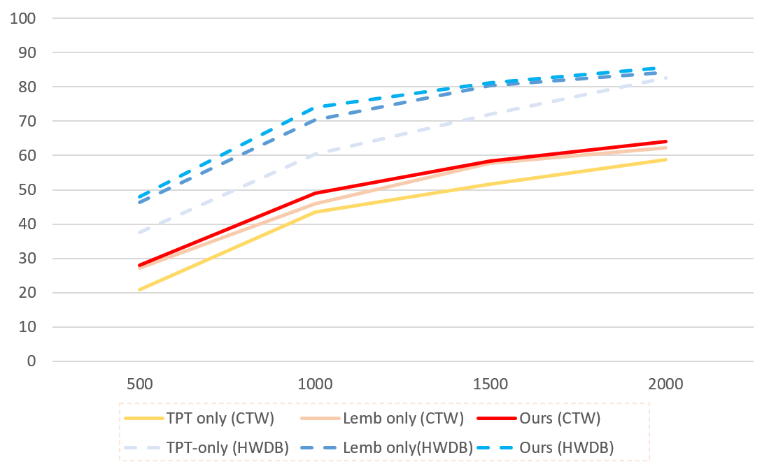
Zero-shot character recognition is a special case of open-set text recognition, where , , and the lengths of all samples equal to one. Here, we benchmark our framework on the HWDB [19] dataset and the CTW [45] dataset to provide a referenced comparison over the capability to recognize NIC characters (Table 2), following the zero-shot Chinese character recognition community. The HWDB dataset is a single-character hand-written dataset collected from writers. We use the HWDB 1.0-1.2 for training and the ICDAR13 competition dataset for evaluation. The CTW dataset is a scene text recognition dataset with character-level annotations. This dataset is more difficult than HWDB due to noise, complex background patterns, and low contrast. In this work, Zhang et al.’s [4] split scheme for training and evaluation labels is adopted to achieve fair comparisons. 121212As they do not release their exact split, we spilt the datasets according to their paper and our exact splits can be referred to our released source codes. For the HWDB dataset, we first randomly split labels (characters) as the evaluation character-set , and then randomly sample , , , and labels from the remaining as the training character-set . On the CTW dataset, we first split characters for testing and then randomly sample , , , and characters for training.
| Accuracy (%) | |||||||||
| HWDB | CTW | ||||||||
| Method | Venue | # characters in training set | # characters in training set | ||||||
| 500 | 1000 | 1500 | 2000 | 500 | 1000 | 1500 | 2000 | ||
| CM* [1] | ICDAR’19 | 44.68 | 71.01 | 80.49 | 86.73 | - | - | - | - |
| DenseRan [39] | ICFHR’18 | 1.70 | 8.44 | 14.71 | 63.8 | 0.12 | 1.50 | 4.95 | 10.08 |
| FewRan [37] | PRL’19 | 33.6 | 41.5 | 63.8 | 70.6 | 2.36 | 10.49 | 16.59 | 22.03 |
| HCCR [4] | PR’20 | 33.71 | 53.91 | 66.27 | 73.42 | 23.53 | 38.47 | 44.17 | 49.79 |
| Ours | - | 47.92 | 74.02 | 81.11 | 85.72 | 28.03 | 49.00 | 58.37 | 64.03 |
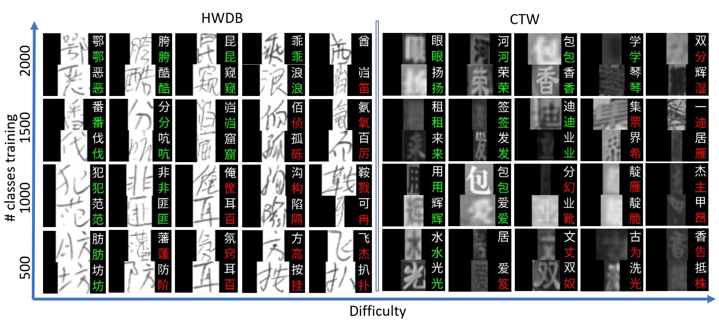
Quantitative performances are shown in Table 2, and qualitative results are shown in Fig. 5. Results demonstrate decent robustness on novel characters for both hand-written and scene characters. Quantitatively, the framework demonstrates more than accuracy advantages compared with a recent method [4] for most setups on both datasets. Similar to other zero-shot methods, the robustness improves as the number of training characters increases, which means a more sufficient sampling on the label space improves performance. Qualitatively, the model can handle a wide range of deterioration while showing some limitations. For handwritten data, the model may fail when a character is written in a cursive way or not correctly written (top-right sample of HWDB in Fig. 5). For scene text data, the model has difficulty recognizing samples with severe blur and low-contrast.
| HWDB | CTW | |||||||
| #NIC | 100 | 200 | 400 | 500 | 50 | 100 | 200 | 250 |
| #NOC | 900 | 800 | 600 | 500 | 450 | 400 | 300 | 250 |
| A(NIC) | 93.5 | 93.9 | 91.0 | 90.0 | 79.3 | 77.1 | 72.6 | 69.6 |
| R(NOC) | 48.0 | 24.6 | 7.9 | 5.1 | 73.3 | 54.7 | 37.7 | 31.5 |
| P(NOC) | 99.7 | 99.5 | 97.9 | 96.7 | 98.9 | 95.9 | 92.4 | 88.6 |
| F(NOC) | 64.8 | 39.5 | 14.6 | 9.7 | 84.2 | 69.7 | 53.5 | 46.5 |
We also extend these tasks to measure the open-set performance by further splitting different fractions of the evaluation characters into as NOC. The performances on the extended tasks are shown in Table 3. Results show that our framework has some extent of rejection capability on both datasets. On the other hand, the number of classes has a negative impact on the rejection capability and recognition accuracy, which is also a common limitation in open-set recognition methods [10].
Summarily, our proposed framework achieves significant advantages on all datasets and setups against most of the state-of-the-art methods, and further provides some extent of rejection capability on “out-of-set” characters. The framework also demonstrates competitive generalization ability against radical-based methods, justifying the feasibility to use glyphs as side information. Unlike radical-based frameworks, our method does not exploit any language-specific priors, thus not restricted to specific languages. As we only use the Noto-sans-regular font for glyphs, obtaining side-information for labels requires much fewer efforts compared to radical-based methods.
| Methods | Venue | Training Set | RNN | IIIT5K | SVT | IC03 | IC13 | CUTE |
|---|---|---|---|---|---|---|---|---|
| AON [6] | CVPR’18 | MJ+ST | Y | 87.0 | 82.8 | 91.5 | - | 76.8 |
| ACE [40] | CVPR’19 | MJ | Y | 82.3 | 82.6 | 89.7 | 82.6 | 82.6 |
| Comb.Best [2] | ICCV’19 | MJ+ST | Y | 87.9 | 87.5 | 94.4 | 92.3 | 71.8 |
| Moran [20] | PR’19 | MJ+ST | Y | 91.2 | 88.3 | 95 | 92.4 | 77.4 |
| SAR [17] | AAAI’19 | MJ+ST | Y | 91.5 | 84.5 | - | - | 83.3 |
| ASTER [31] | PAMI’19 | MJ+ST | Y | 93.4 | 93.6 | 94.5 | 91.8 | 79.5 |
| ESIR [46] | CVPR’19 | MJ+ST | Y | 93.3 | 90.2 | - | - | 83.3 |
| SEED [25] | CVPR’20 | MJ+ST | Y | 93.8 | 89.6 | - | 92.8 | 83.6 |
| DAN [38] | AAAI’20 | MJ+ST | Y | 94.3 | 89.2 | 95.0 | 93.9 | 84.4 |
| Rosetta [3][2] | KDD’18 | MJ+ST | N | 84.3 | 84.7 | 92.9 | 89.0 | 69.2 |
| CA-FCN* [18] | AAAI’19 | ST | N | 92.0 | 82.1 | - | 91.4 | 78.1 |
| TextScanner* [36] | AAAI’20 | MJ+ST+Extra | N | 93.9 | 90.1 | - | 92.9 | 83.3 |
| Ours | - | MJ+ST | N | 90.40 | 83.92 | 91.00 | 90.24 | 82.29 |
| Ours-Large | - | MJ+ST | N | 92.63 | 88.25 | 93.42 | 93.79 | 86.80 |
5.3 Standard Close-Set Text Recognition
Experiments on popular close-set benchmarks are also conducted, and results show that our method suffices as a feasible lightweight method on conventional close-set text recognition tasks. Following the majority of methods in this community, we train our model on synthetic samples from Jaderberg (MJ) [14] and Gupta (ST) [11]. We use the IIIT5K-Words (IIIT5K), Street View Text (SVT), ICDAR 2003 (IC03), ICDAR 2013 (IC13), and CUTE80 (CUTE) as our testing sets. Among the testing sets, IIIT5K, IC03, IC13, and SVT focus on regular shaped texts, and CUTE focuses on irregular-shaped text. IIIT5K contains testing images collected from the web. SVT has testing images from Google Street View. IC03 includes words from scene text, while IC13 extends IC03 and contains images. CUTE80 includes curved samples. All models are trained for epochs for close-set experiments, and the results are shown in Table 4.
On the close-set benchmarks, our regular method is performance-wise better than early lightweight methods like Rosetta [3]. The method is also comparable to the state-of-the-art RNN-free method CA-FCN [18], while being significantly faster. Moreover, our method does not require character-level annotations for training. We also provide a larger model around the speed of CA-FCN [18] yielding better performances close to heavy RNN-based methods [38]. Plus, our methods is RNN-free, hence do not require batching up to margin out the latency caused by RNNs.

Representative samples are illustrated in Fig. 6. Our model demonstrates some extent of robustness for samples with blur, irregular shapes, and different styles. However, due to the absence of RNN modules, the framework lacks sufficient capability of modeling context information, hence showing a tendency to confuse characters that have closer shapes, e.g., ‘s’ and ‘5’.
We also conduct a dictionary-based test to compare with other methods (Table 5). Results show a significant performance advantage compared to Zhang et al.’s method [47], which is the only zero-shot text recognition method that tested on standard close-set recognition benchmarks to our knowledge. Under this setup, the framework is also performance-wise close to SOTA methods like CA-FCN [18].
| Method | Batch size | IIIT5K | CUTE | GPU | TFlops | Speed (ms) | Vram (MB) |
| CRNN* [29] | 1 | 78.2 | — | P40 | 12 | 4.4 | - |
| Rosetta* [3] | 1 | 84.3 | 69.2 | P40 | 12 | 4.7 | - |
| Comb.Best* [2] | 1 | 87.9 | 74.0 | P40 | 12 | 27.6 | - |
| CA-FCN [18] | 1 | 92.0 | 79.9 | Titan XP | 12 | 22.2 | - |
| Ours | 1 | 90.40 | 82.29 | RTX2070M | 6.6 | 9.19 | 1227 |
| Ours | 16 | 90.40 | 82.29 | RTX2070M | 6.6 | 4.68 | 1519 |
| Ours-Large | 1 | 92.63 | 86.80 | RTX2070M | 6.6 | 14.18 | 1377 |
| Ours-Large | 16 | 92.63 | 86.80 | RTX2070M | 6.6 | 7.81 | 1663 |
The speeds of our framework with different model sizes and batch sizes are shown in Table 6. Speeds reported by other methods are also listed as a rough reference. Our models run with FP32 datatype on an RTX2070 Mobile GPU, and the speeds are computed on the IIIT5k dataset. For maximum throughput, our method can reach a FPS running multi-batched. For latency critique tasks, our method can manage a ms latency under single-batched mode on the GPU of around TFLOPS. Space-wise, our models do not require much VRAM either. In summary, our model is reasonably small and fast, thus friendly to smaller devices like laptops, phones, and single-boards.
In conclusion, despite showing an acceptable margin against heavy SOTA methods, the framework is comparable to, or better than many popular RNN-free methods for close-set text recognition. Our framework demonstrates much more readiness to replace conventional text recognition methods in real-world applications, compared to other zero-shot text recognition methods like [47].
5.4 Open-Set Text Recognition
In this section, we report the performance of the large model under five different splits, namely the GZSL mode, the OSR mode (w/o SOC), the OSR mode (with SOC), the GOSR mode, and the OSTR mode. The results and specifics of each split are shown in Table 7. The model shows overall acceptable recognition capability for seen and novel characters under most scenarios. For the rejection capability, the performance goes well with seen characters (SOC). The performance is also acceptable for some novel characters which are structural-wise close to characters in training set. However, the model demonstrates major limitations on the scalability over class number of . However, the precision of the framework is above 60% on all setups, meaning human labor necessary to dismiss fake warnings is low. Considering most applications involves a large amount of data and each novel character only needs to be spotted once, the weakness on recall is not of much importance. Hence, the framework is still feasible for finding out novel characters in the data-stream.
| Name | LA | R | P | F | |||
| GZSL | Unique Kanji, Shared Kanji, Kana, Latin | 1460 | 30.83 | - | - | - | |
| OSR w/o SOC | Shared Kanji, Latin | Unique Kanji, Kana | 849 | 74.35 | 11.27 | 98.28 | 20.23 |
| OSR with SOC | Shared Kanji | Unique Kanji, Kana, Latin | 787 | 80.28 | 25.15 | 99.26 | 40.13 |
| GOSR | Shared Kanji, Unique Kanji, Latin | Kana | 1301 | 56.03 | 3.03 | 63.52 | 5.78 |
| OSTR | Shared Kanji, Unique Kanji | Kana, Latin | 1239 | 58.57 | 24.46 | 93.78 | 38.80 |

| Name | Sample Requires | Sample Excludes | CA(%) | LA(%) |
| Shared Kanji | Shared Kanji | Unique Kanji, Kana | 85.69 | 73.21 |
| Unique Kanji | Unique Kanji | Kana | 76.50 | 40.87 |
| All Kanji | Unique Kanji or Shared Kanji | Kana | 79.94 | 54.91 |
| Kana | Hiragana or Katakana | 25.10 | 0.72 | |
| All | 54.03 | 30.83 |
In this work, we primarily focus on implementing the language-agnostic recognition capability of unseen labels, so we primarily analyze the detailed performance over the GZSL spilt. Specifically, qualitative samples are shown in Fig. 7, and a detailed breakdown of the large model is listed in Table 8. In the table, “Sample Requires” indicates each sample must include at least one type among the listed, while “Sample Excludes” refers to each sample that cannot include any of the listed types of characters. “Shared Kanji” refers to Kanjis covered by the Tier-1 Simplified Chinese characters [19], while “Unique Kanji” means unseen Kanjis that are novel to the model. Despite showing reasonable robustness on the unique Kanjis, our framework shows limited generalization capability on Hiragana and Katakana characters.


Note the size of the character-set can lay a serious impact on recognition performance. E.g., Row 2 and Row 3 in Table 7 report higher LAs than Row 1 and Row 3 in Table 8 for having a smaller . This phenomenon suggests the decision boundaries of different prototypes may overlap with each other despite being bounded by the threshold . Worth mentioning, that the result is not directly comparable to the zero-shot character recognition results on the CTW dataset due to the vast differences among datasets, character-sets, and metrics.
To further validate the generalization capability of the large model, we conducted evaluations on word-level samples from Korean, Russian, and Greek. The Korean words are drawn from the MLT dataset like the Japanese language, and qualitative results are shown in Fig. 8. Quantitative-wise, the method shows % Character Accuracy and % Line Accuracy on Korean words, where the main limitation comes from confusion over characters with close shapes. For the Russian and the Greek language, we collected the samples from the SIW-13 [28] dataset. As the dataset does not provide annotation on contents, we only demonstrate the qualitative results in Fig 9.
5.5 Ablative Studies
To validate the robustness of the proposed modules, we performed extensive ablative studies on all three tasks, i.e., zero-shot Chinese character recognition, close-set text recognition, and open-set text recognition.
We first perform ablative studies on the zero-shot character recognition benchmarks to validate the feasibility of on improving the generalization ability. Parameters and set-ups are the same as the ones in the above experiments. Results (Fig. 10) show that improves the performance significantly, especially with less training data. Our assumption is, that pushing prototypes apart makes the ProtoCNN more detail-sensitive, hence more robust to potential confusions caused by characters with similar shapes. Additionally, the experiments also show that the topology-preserving transformation provides a limited improvement on character recognition tasks. The reason could be precisely located characters are less prone to geometry deteriorations.
| Method | TPT | IIIT5K | SVT | IC03 | IC13 | CUTE | |
|---|---|---|---|---|---|---|---|
| Ours-Large | ✓ | ✓ | 92.63 | 88.25 | 93.42 | 93.79 | 86.60 |
| Ours-Large w/o TPT | ✓ | 91.80 | 86.08 | 92.84 | 92.21 | 81.94 |
We then perform ablative studies to validate the effectiveness of the proposed topology-preserving transformation (TPT) in scene text recognition. Results show that the TPT module yields a noticeable improvement on most datasets under the large configuration. Noticeably, TPT yields significant improvement on the CUTE dataset, which contains a lot of irregular-shaped text.
| Method | TPT | L2P | LA | LA-large | |
|---|---|---|---|---|---|
| Ours | ✓ | ✓ | ✓ | 28.11 | 30.83 |
| Ours w/o TPT | ✓ | ✓ | 27.56 | 30.35 | |
| Ours w/o | ✓ | ✓ | 24.89 | 29.23 | |
| Conventional | ✓ | - | 17.63 | 18.05 |
Finally, we perform ablative studies on the proposed open-set text recognition, with results shown in Table 10. Module-wise, both the proposed topology-preserving transformation (TPT) and the prototype regularization term () improve the recognition performance on the open-set challenge. Framework-wise, the full framework yields significantly better performance against the conventional method over both character accuracy and line accuracy. Here, the conventional method replaces the label-to-prototype module and the open-set predictor with a linear classifier, pipeline-wise similar to an RNN-free version of DAN [38]. This indicates our framework achieves reasonable recognition capability over novel characters without sacrificing much close-set performance.
In summary, our label-to-prototype learning framework achieves competitive performance on novel characters without sacrificing much of the close-set performances. The topology-preserving transformation module shows robust improvement on all setups in all three tasks. The regularization term also shows steady improvements on novel characters, potentially by improving the inter-class distance on the prototype space, leaving more space for novel classes.

6 Limitation
The major problem of our framework is the limited robustness over domain bias, e.g, the performance drop on Hiragana and Katakana. Possibly due to the significant visual differences between Kanas and characters in the training set. Specifically, Kanas reside in an under-sampled subspace on the template space , which consequentially leads to larger “errors” in generated prototypes. This assumption can also be backed by the t-SNE [35] visualization of generated prototypes (shown in Fig. 11). We can see that Kanas gather in the left-most region of the oval spanned by the training set characters (gray dots), while most other novel characters like Unique Kanjis are distributed relatively evenly in the space. Since the network training is a function fitting process, the points from less-sufficiently sampled regions tend to have larger fitting errors. In this case, the under-sampling problem causes bad class centers and visual features, resulting in lower recognition accuracy of Kanas and Korean Hanguls.
7 Conclusions
We propose a novel framework for the open-set text recognition task via label-to-prototype learning. Results show a largely improved performance compared with state-of-the-art methods on zero-shot character recognition tasks. Our framework also reaches competitive performance on the conventional close-set text line recognition benchmarks, demonstrating its readiness for applications. Moreover, our method draws a strong baseline on the open-set text recognition task with a large character-set and complex deterioration. In summary, our method can robustly handle isolated characters and text lines in both open-set and close-set scenarios.
Despite showing impressive generalization capability on open-set scenarios, our framework still has some limitations. Specifically, our method tends to fail to recognize characters that have significantly different shapes from the seen characters (e.g., Kanas and Hanguls). Domain adaption techniques may be investigated to solve the domain bias among complex characters and different languages in future research. Also, despite showing some extent of rejection capability, the model still has much room to improve. This makes another topic of our future research.
8 Acknowledgement
The research is partly supported by the National Key Research and Development Program of China (2020AAA09701), The National Science Fund for Distinguished Young Scholars (62125601), and the National Natural Science Foundation of China (62006018, 62076024).
References
- [1] Xiang Ao, Xu-Yao Zhang, Hong-Ming Yang, Fei Yin, and Cheng-Lin Liu. Cross-modal prototype learning for zero-shot handwriting recognition. In ICDAR, pages 589–594. IEEE, 2019.
- [2] Jeonghun Baek, Geewook Kim, Junyeop Lee, Sungrae Park, Dongyoon Han, Sangdoo Yun, Seong Joon Oh, and Hwalsuk Lee. What is wrong with scene text recognition model comparisons? dataset and model analysis. In ICCV, pages 4714–4722, 2019.
- [3] Fedor Borisyuk, Albert Gordo, and Viswanath Sivakumar. Rosetta: Large scale system for text detection and recognition in images. In KDD, pages 71–79, 2018.
- [4] Zhong Cao, Jiang Lu, Sen Cui, and Changshui Zhang. Zero-shot handwritten chinese character recognition with hierarchical decomposition embedding. Pattern Recognition, 107:107488, 2020.
- [5] Jingye Chen, Bin Li, and Xiangyang Xue. Zero-shot chinese character recognition with stroke-level decomposition. In IJCAI, pages 615–621, 2021.
- [6] Zhanzhan Cheng, Yangliu Xu, Fan Bai, Yi Niu, Shiliang Pu, and Shuigeng Zhou. AON: towards arbitrarily-oriented text recognition. In CVPR, pages 5571–5579, 2018.
- [7] Chee Kheng Chng, Errui Ding, Jingtuo Liu, Dimosthenis Karatzas, Chee Seng Chan, Lianwen Jin, Yuliang Liu, Yipeng Sun, Chun Chet Ng, Canjie Luo, Zihan Ni, ChuanMing Fang, Shuaitao Zhang, and Junyu Han. ICDAR2019 robust reading challenge on arbitrary-shaped text - rrc-art. In ICDAR, pages 1571–1576. IEEE, 2019.
- [8] Jifeng Dai, Haozhi Qi, Yuwen Xiong, Yi Li, Guodong Zhang, Han Hu, and Yichen Wei. Deformable convolutional networks. In ICCV, pages 764–773. IEEE Computer Society, 2017.
- [9] Geli Fei and Bing Liu. Breaking the closed world assumption in text classification. In Kevin Knight, Ani Nenkova, and Owen Rambow, editors, NAACL, pages 506–514. The Association for Computational Linguistics, 2016.
- [10] Chuanxing Geng, Sheng-Jun Huang, and Songcan Chen. Recent advances in open set recognition: A survey. IEEE Trans. Pattern Anal. Mach. Intell., 43(10):3614–3631, 2021.
- [11] Ankush Gupta, Andrea Vedaldi, and Andrew Zisserman. Synthetic data for text localisation in natural images. In CVPR, pages 2315–2324, 2016.
- [12] Kaiming He, Xiangyu Zhang, Shaoqing Ren, and Jian Sun. Deep residual learning for image recognition. In CVPR, pages 770–778, 2016.
- [13] Yuhao Huang, Lianwen Jin, and Dezhi Peng. Zero-shot chinese text recognition via matching class embedding. In ICDAR, volume 12823, pages 127–141, 2021.
- [14] Max Jaderberg, Karen Simonyan, Andrea Vedaldi, and Andrew Zisserman. Synthetic data and artificial neural networks for natural scene text recognition. CoRR, abs/1406.2227, 2014.
- [15] Siwei Lai, Liheng Xu, Kang Liu, and Jun Zhao. Recurrent convolutional neural networks for text classification. In Blai Bonet and Sven Koenig, editors, Proceedings of the Twenty-Ninth AAAI Conference on Artificial Intelligence, January 25-30, 2015, Austin, Texas, USA, pages 2267–2273. AAAI Press, 2015.
- [16] Junyeop Lee, Sungrae Park, Jeonghun Baek, Seong Joon Oh, Seonghyeon Kim, and Hwalsuk Lee. On recognizing texts of arbitrary shapes with 2d self-attention. In CVPR, pages 2326–2335. IEEE, 2020.
- [17] Hui Li, Peng Wang, Chunhua Shen, and Guyu Zhang. Show, attend and read: A simple and strong baseline for irregular text recognition. In AAAI, pages 8610–8617, 2019.
- [18] Minghui Liao, Jian Zhang, Zhaoyi Wan, Fengming Xie, Jiajun Liang, Pengyuan Lyu, Cong Yao, and Xiang Bai. Scene text recognition from two-dimensional perspective. In AAAI, pages 8714–8721, 2019.
- [19] Cheng-Lin Liu, Fei Yin, Da-Han Wang, and Qiu-Feng Wang. CASIA online and offline chinese handwriting databases. In ICDAR, pages 37–41. IEEE Computer Society, 2011.
- [20] Canjie Luo, Lianwen Jin, and Zenghui Sun. MORAN: A multi-object rectified attention network for scene text recognition. Pattern Recognition, 90:109–118, 2019.
- [21] Sarah Parisot, Pedro M. Esperança, Steven McDonagh, Tamas J. Madarasz, Yongxin Yang, and Zhenguo Li. Long-tail recognition via compositional knowledge transfer. In CVPR, 2022.
- [22] Tristan Postadjian, Arnaud Le Bris, Clément Mallet, and Hichem Sahbi. Superpixel partitioning of very high resolution satellite images for large-scale classification perspectives with deep convolutional neural networks. In IGARSS, pages 1328–1331, 2018.
- [23] Farhad Pourpanah, Moloud Abdar, Yuxuan Luo, Xinlei Zhou, Ran Wang, Chee Peng Lim, and Xi-Zhao Wang. A review of generalized zero-shot learning methods. CoRR, abs/2011.08641, 2020.
- [24] Hang Qi, Matthew Brown, and David G. Lowe. Low-shot learning with imprinted weights. In CVPR, pages 5822–5830. IEEE Computer Society, 2018.
- [25] Zhi Qiao, Yu Zhou, Dongbao Yang, Yucan Zhou, and Weiping Wang. SEED: semantics enhanced encoder-decoder framework for scene text recognition. In CVPR, pages 13525–13534, 2020.
- [26] Walter J. Scheirer, Anderson de Rezende Rocha, Archana Sapkota, and Terrance E. Boult. Toward open set recognition. IEEE Trans. Pattern Anal. Mach. Intell., 35(7):1757–1772, 2013.
- [27] Fenfen Sheng, Zhineng Chen, and Bo Xu. NRTR: A no-recurrence sequence-to-sequence model for scene text recognition. In ICDAR, pages 781–786. IEEE, 2019.
- [28] Baoguang Shi, Xiang Bai, and Cong Yao. Script identification in the wild via discriminative convolutional neural network. Pattern Recognit., 52:448–458, 2016.
- [29] Baoguang Shi, Xiang Bai, and Cong Yao. An end-to-end trainable neural network for image-based sequence recognition and its application to scene text recognition. IEEE Trans. Pattern Anal. Mach. Intell., 39(11):2298–2304, 2017.
- [30] Baoguang Shi, Xinggang Wang, Pengyuan Lyu, Cong Yao, and Xiang Bai. Robust scene text recognition with automatic rectification. In CVPR, pages 4168–4176, 2016.
- [31] Baoguang Shi, Mingkun Yang, Xinggang Wang, Pengyuan Lyu, Cong Yao, and Xiang Bai. ASTER: an attentional scene text recognizer with flexible rectification. IEEE Trans. Pattern Anal. Mach. Intell., 41(9):2035–2048, 2019.
- [32] Baoguang Shi, Cong Yao, Minghui Liao, Mingkun Yang, Pei Xu, Linyan Cui, Serge J. Belongie, Shijian Lu, and Xiang Bai. ICDAR2017 competition on reading chinese text in the wild (RCTW-17). In ICDAR, pages 1429–1434. IEEE, 2017.
- [33] Mohamed Ali Souibgui, Alicia Fornés, Yousri Kessentini, and Beáta Megyesi. Few shots is all you need: A progressive few shot learning approach for low resource handwriting recognition. CoRR, abs/2107.10064, 2021.
- [34] Yipeng Sun, Dimosthenis Karatzas, Chee Seng Chan, Lianwen Jin, Zihan Ni, Chee Kheng Chng, Yuliang Liu, Canjie Luo, Chun Chet Ng, Junyu Han, Errui Ding, and Jingtuo Liu. ICDAR 2019 competition on large-scale street view text with partial labeling - RRC-LSVT. In ICDAR, pages 1557–1562. IEEE, 2019.
- [35] Laurens Van der Maaten and Geoffrey Hinton. Visualizing data using t-sne. Journal of machine learning research, 9(11), 2008.
- [36] Zhaoyi Wan, Minghang He, Haoran Chen, Xiang Bai, and Cong Yao. Textscanner: Reading characters in order for robust scene text recognition. In AAAI, pages 12120–12127, 2020.
- [37] Tianwei Wang, Zecheng Xie, Zhe Li, Lianwen Jin, and Xiangle Chen. Radical aggregation network for few-shot offline handwritten chinese character recognition. Pattern Recognition Letters, 125:821–827, 2019.
- [38] Tianwei Wang, Yuanzhi Zhu, Lianwen Jin, Canjie Luo, Xiaoxue Chen, Yaqiang Wu, Qianying Wang, and Mingxiang Cai. Decoupled attention network for text recognition. In AAAI, pages 12216–12224, 2020.
- [39] Wenchao Wang, Jianshu Zhang, Jun Du, Zi-Rui Wang, and Yixing Zhu. Denseran for offline handwritten chinese character recognition. In ICFHR, pages 104–109, 2018.
- [40] Zecheng Xie, Yaoxiong Huang, Yuanzhi Zhu, Lianwen Jin, Yuliang Liu, and Lele Xie. Aggregation cross-entropy for sequence recognition. In CVPR, pages 6538–6547, 2019.
- [41] Hong-Ming Yang, Xu-Yao Zhang, Fei Yin, and Cheng-Lin Liu. Robust classification with convolutional prototype learning. In CVPR, pages 3474–3482, 2018.
- [42] Hong-Ming Yang, Xu-Yao Zhang, Fei Yin, Qing Yang, and Cheng-Lin Liu. Convolutional prototype network for open set recognition. IEEE Transactions on Pattern Analysis and Machine Intelligence, 2020.
- [43] Mingkun Yang, Yushuo Guan, Minghui Liao, Xin He, Kaigui Bian, Song Bai, Cong Yao, and Xiang Bai. Symmetry-constrained rectification network for scene text recognition. In CVPR, pages 9146–9155, 2019.
- [44] Deli Yu, Xuan Li, Chengquan Zhang, Tao Liu, Junyu Han, Jingtuo Liu, and Errui Ding. Towards accurate scene text recognition with semantic reasoning networks. In CVPR, pages 12110–12119, 2020.
- [45] Tai-Ling Yuan, Zhe Zhu, Kun Xu, Cheng-Jun Li, Tai-Jiang Mu, and Shi-Min Hu. A large chinese text dataset in the wild. J. Comput. Sci. Technol., 34(3):509–521, 2019.
- [46] Fangneng Zhan and Shijian Lu. ESIR: end-to-end scene text recognition via iterative image rectification. In CVPR, pages 2059–2068, 2019.
- [47] Chuhan Zhang, Ankush Gupta, and Andrew Zisserman. Adaptive text recognition through visual matching. In ECCV, volume 12361 of Lecture Notes in Computer Science, pages 51–67, 2020.
- [48] Hanlei Zhang, Hua Xu, and Ting-En Lin. Deep open intent classification with adaptive decision boundary. In IAAI, pages 14374–14382. AAAI Press, 2021.
- [49] Jianshu Zhang, Jun Du, and Lirong Dai. Radical analysis network for learning hierarchies of chinese characters. Pattern Recognit., 103:107305, 2020.
| Name | Distance | Training Template | Evaluation Template | A | R | P | F | |
|---|---|---|---|---|---|---|---|---|
| Ours | DotProd | Sans | Sans | 500 | 65.53 | - | - | - |
| Ours-X | DotProd | Sans | Serif | 500 | 53.52 | - | - | - |
| MF-A | DotProd | Sans+Serif | Sans | 500 | 66.79 | - | - | - |
| MF-B | DotProd | Sans+Serif | Serif | 500 | 66.72 | - | - | - |
| Cos | Cosine | Sans | Sans | 500 | 59.53 | - | - | - |
| Ours | DotProd | Sans | Sans | 250 | 70.62 | 33.34 | 88.00 | 48.36 |
| Ours-X | DotProd | Sans | Serif | 250 | 59.50 | 42.01 | 76.98 | 54.35 |
| MF-A | DotProd | Sans+Serif | Sans | 250 | 69.89 | 30.94 | 85.63 | 45.46 |
| MF-B | DotProd | Sans+Serif | Serif | 250 | 68.03 | 28.64 | 84.17 | 42.73 |
| Cos | Cosine | Sans | Sans | 250 | 65.66 | 11.32 | 85.21 | 20.00 |
Appendix A
In this section, we discuss other factors that affect recognition performance, namely the fonts used for templates, the metric used, and the number of characters in . Note the performance is a little bit different as the results are from another run on a faster device. For font selection for templates, we train the model with both Noto-sans and Noto-serif and test with each font (MF-A and MF-B). Extra fonts does not yield noticeable performance change, presumably due to the increased training variance. “Ours-X” evaluates the “Ours” model trained with Sans font with Serif font, yielding a significant performance degrade due to the shift on class centers. The rejection rate also increased due to the center shift, resulting in a higher recall and lower precision. For distance metric, we implement the scaled cosine metric according to Parisot et al. [21], however, the performance is not ideal. We will attempt to figure out the reason in the future. As we can see in Table 3, the scalability of this method is limited like many classification methods, which is a common issue in the classification domain.
Appendix B

In this section, we explain the reasons behind the definition of open-set text recognition, and corresponding use cases in real-life applications show in Figure 12. With the openness and fast-evolving nature of the internet, the character set of the incoming dataset can change over time. The volatile property of the character set also applies to historical document recognition as previously unknown characters could be found from the samples. In a word, the two main goals of the OSTR task are reducing adaption cost and achieving active novel characters spotting from the data stream.
Considering the majority of samples in real-life applications still involve seen characters, the task demands recognition capability of SIC like conventional close-set text recognition [2]. However, close-set methods require a data collection (synthetic or annotation) and retraining process on each character set change. Generally speaking, the retraining process would cost around several GPU days, depending on the amount of data and model size. For the internet-oriented data, the cost could be hefty as the changes may occur frequently, under the pretext of the booming trend of mixing emojis with normal characters, and emojis happen to evolve constantly. On the other hand, for historical data where annotation could be expensive and synthetic data can be limited due to insufficient amount of available fonts, rendering the conventional pipeline less feasible. To reduce the adaption cost, we introduce the recognition capability of NIC like zero-shot tasks [37, 47].
Furthermore, in real applications we do not know what novel characters we may encounter, nor do we know when. Hence, as a result of lacking rejection capability, the conventional close-set and zero-shot text recognition methods would need to wait till end-users (OCR service subscribers) complain before the sysadmins (OCR service providers) can notice the novel characters. To address this problem, we introduce the rejection capability over NOC characters like OSR tasks [10]. Here we further extend the subjects to seen classes (SOC) as well. One main reason is, that some characters or emoticons may get temporarily obsolete and become less frequently used. In this case, the user may want to remove them from the character set to speed up, while not risking missing and mistaking them for something else when they re-appear. Hence, we naturally extend the subject of rejection to include both SOC and NOC.
Summing up, the OSTR task demands the capability to match samples with side-information of an arbitrary set of classes for recognition, and reject samples failing matching any classes in the set. Noteworthy, the task still demands close-set recognition performance, hence the sysadmins still retain the option to retrain an OSTR method with collected data. Furthermore, an OSTR method offers extra options of using a quick patch as a temporary (till retraining is done) or permanent (no retraining at all) solution.
Appendix C
As this paper involves a lot of notions, we collect scalars in Table 12, sets in Table 13, and other notations in Table 14. Each table illustrates the notations with their shapes, first appearances, and corresponding short descriptions.
| Notation | Occurrence | Type | Shape / Value | Description |
|---|---|---|---|---|
| Ch. 4.1 | const | # dimensions of the prototype space, 512 in this work | ||
| Ch 4.2 | const | Limits extent of rectification the TPT module can do | ||
| Ch 4.5 | const | The fraction of seen characters for the label sampler | ||
| Ch 4.5 | const | The maximum of the training process | ||
| Ch. 5.1 | const | The maximum sample length the model supports(including end of speech token). | ||
| Ch 4.5 | const | Weight of | ||
| Ch.5.1 | const | The maximum iteration of the training process | ||
| Ch 4.2 | index | indicates a timestamp (the item) | ||
| Ch 4.1 | scalar | the upper bound of timestamp length | ||
| Ch.4.4 | scalar | Traiable decision boundary radius for all classes | ||
| Ch.4.5 | loss | The embedding loss pusing prototypes too close too close to each other away. | ||
| Ch.4.5 | loss | The total loss of the proposed method | ||
| Ch.4.5 | loss | The cross entropy of the classification task. | ||
| Ch. 2.1 | metric | Line accuracy | ||
| Ch. 2.1 | metric | Char accuracy | ||
| Ch. 2.1 | metric | Recall of spotting samples containing . | ||
| Ch. 2.1 | metric | Precision of spotting samples containing . | ||
| Ch. 2.1 | metric | Fmeasure of spotting samples containing . | ||
| Ch4.3 | character | A character in |
| Notation | Occurrence | Type | Element Shape | Description |
| Ch. 4.1 | space | Set of all characters. | ||
| Ch. 4.1 | space | Template space containing gray scale patches from the Noto-font (or other fonts). | ||
| Ch. 4.1 | space | Set of all characters. | ||
| Ch.2.1 | set | Label strings(ground truths) of samples a dataset. | ||
| Ch.2.1 | set | Prediction results of samples a dataset. | ||
| Ch. 2.1 | set | Set of distinct character(label) in the training set | ||
| Ch. 2.1 | set | Set of distinct character(label) in the testing set | ||
| Ch. 2.1 | set | Labels in the testing set with side-information. | ||
| Ch. 2.1 | set | Out-of-set labels in the testing set without side-information. | ||
| Ch.4.5 | set | The set of characters appear in a batch of training data | ||
| Ch.4.5 | set | The set of active labels in each training iteration, | ||
| Ch.4.5 | set | Sampled labels that appear in the batch of training data | ||
| Ch.4.5 | set | Sampled labels that does not appear in the batch of training data | ||
| Ch. 4.1 | set | An arbitary Set of characters. | ||
| set | All templates of the character, each corresponds to a case. |
| Notation | Occurrence | Type | “Shape” | Description |
|---|---|---|---|---|
| Ch. 2.1 | function | return 1 if the two inputs are the same, 0 otherwise | ||
| Ch 2.1 | function | Edit distance between strings. | ||
| Ch 2.1 | function | Returns the length of the string. | ||
| Ch 2.1 | function | Indicator function returns whether the string contains “out-of-set” characters in . | ||
| Ch 4.3 | function | Mapping template to a normalized prototype. | ||
| Ch 4.3 | function | Mapping a character label to all corresponding templates, each templates is a gray scale patch of one case of the character. | ||
| Ch 4.3 | function | Mapping template to a normalized prototype. | ||
| Ch. 4.1 | tensor | Prototypes for all classes. Note one class can be mapped to more than one prototypes depending on the number of cases. | ||
| Ch 4.2 | tensor | An (intermediate) feature map of the input word clip. | ||
| Ch 4.2 | tensor | The foreground density matrix for the -axis. | ||
| Ch 4.2 | tensor | The foreground density matrix for the -axis. | ||
| Ch 4.2 | tensor | The coordination mapping for the rectification. | ||
| Ch4.1 | tensor | The feature of each character in one sample. indicates the length of the sample. | ||
| Ch4.3 | tensor | A template on the template space . | ||
| Ch4.3 | tensor | A prototype of a “case” from a character. | ||
| Ch 4.4 | tensor | Similarity of character feature at each timestamp and each prototype. | ||
| Ch 4.4 | tensor | Similarity of character feature at each timestamp and each character. | ||
| Ch 4.4 | tensor | Final score of character feature at each timestamp (added the score for unknown character). |