Towards Kriging-informed Conditional Diffusion for Regional Sea-Level Data Downscaling
Abstract.
Given coarser-resolution projections from global climate models or satellite data, the downscaling problem aims to estimate finer-resolution regional climate data, capturing fine-scale spatial patterns and variability. Downscaling is any method to derive high-resolution data from low-resolution variables, often to provide more detailed and local predictions and analyses. This problem is societally crucial for effective adaptation, mitigation, and resilience against significant risks from climate change. The challenge arises from spatial heterogeneity and the need to recover finer-scale features while ensuring model generalization. Most downscaling methods (Li et al., 2020) fail to capture the spatial dependencies at finer scales and underperform on real-world climate datasets, such as sea-level rise. We propose a novel Kriging-informed Conditional Diffusion Probabilistic Model (Ki-CDPM) to capture spatial variability while preserving fine-scale features. Experimental results on climate data show that our proposed method is more accurate than state-of-the-art downscaling techniques.
1. Introduction
Given coarse-resolution climate projections from global climate models or satellite data, the problem of statistical downscaling aims to estimate high-resolution regional climate data, capturing fine-scale spatial patterns and variability for a climate variable (e.g., sea-level rise). Since downscaling generates high-resolution data from low-resolution variables, statistical downscaling uses statistical methods to establish relationships between coarse-resolution climate data and high-resolution historical observations. For instance, Figure 1 shows a geographic area near Ecuador and Peru in two different time frames. In both images, the blurry coarse-resolution projections display limited variation in sea surface height anomalies compared to the fine-scale resolution, as shown in the rectangular strips (in red). The ability to capture localized variations is crucial for accurately predicting climate change effects (e.g., sea-level rise) in a specific area.
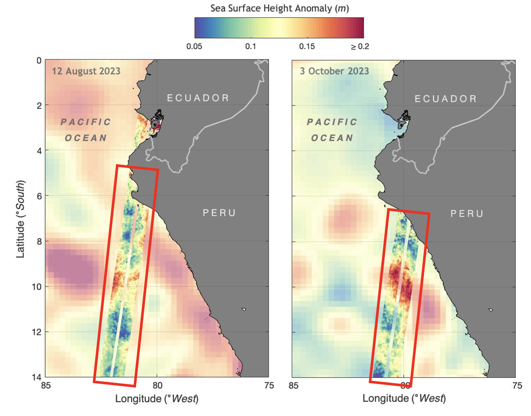
An illustration showing the difference between coarse resolution and fine-scale resolution observations.
The regional downscaling problem is vital for developing comprehensive climate policies and strategies. The impacts of climate change, as predicted by global climate models, range from extreme weather events to rises in sea levels and shifts in agricultural productivity. Enhancing the spatial precision of climate data is vital for accurately assessing risks in specific regions. Decision-makers require such information to strategize how communities can successfully mitigate and adapt to these threats. For example, coastal areas worldwide face severe risks associated with sea-level rise, where even small changes can lead to significant flooding, erosion, and habitat loss (Intergovernmental Panel on Climate Change (2021), IPCC; Rabinowitz et al., 2023). High-resolution data contributes to accurate regional predictions of this risk, essential for effective coastal management, infrastructure planning, and disaster preparedness.
| Application Domain | Occurrence of Spatial Variability |
|---|---|
| Temperature | Regional Temperature Change Prediction |
| Soil Carbon Emission | Local Farmland Emission vs Global |
| Precipitation | Regional variability in precipitation |
| Extreme wind | Regional wind variability (e.g., wind farms) |
| Climate Policy Making | County vs State level jurisdictions. |
The problem of statistical downscaling in climate data is challenging due to climate data’s inherent complexity and variability involving intricate spatial and temporal dependencies influenced by numerous physical processes (e.g., ocean currents, wind patterns, temperature gradients, and coastal topography). The non-stationarity of climate data, driven by dynamic changes in climate patterns and extreme events, further complicates the development of reliable and robust downscaling techniques. For example, statistical properties like mean and standard deviation may not be constant over time (Liu et al., 2022; Church et al., 2013).
Traditional Kriging and interpolation-based methods (Vicente-Serrano et al., 2014; Teutschbein and Seibert, 2012; Maraun et al., 2018) for downscaling sea-level rise data often fall short due to their reliance on stationarity assumptions and their inability to capture the dynamic nature of climate data. These methods typically smooth the data excessively, resulting in the loss of critical fine-scale features. The loss leads to an inaccurate representation of the underlying physical processes, such as ocean currents, wind patterns, and temperature gradients. On the other hand, machine learning-based methods (Watt and Mansfield, 2024; Leinonen, 2020; Wan et al., 2023), while powerful in capturing non-linear relationships, often struggle with generalization and maintaining physical consistency. These models can be data-hungry and sensitive to the quality and quantity of training data.
Traditional super-resolution models, designed primarily for image processing, cannot be directly applied to climate downscaling for the following reasons. (a) They lack physical constraints and fail to incorporate the complex, nonlinear relationships between various components of the Earth system (Oppenheimer et al., 2019; Garner et al., 2018). (b) They do not handle the high-dimensional nature of climate data effectively and often require large amounts of high-resolution training data, typically sparse in climate science (Wang et al., 2021). (c) They are deterministic and do not provide probabilistic outputs or uncertainty estimates, which are crucial for climate predictions (McGranahan et al., 2007). (d) They lack generalization across different regions and periods, as they do not account for the multiple scales inherent in climate processes (Kopp et al., 2014).
To address these limitations, we propose a Kriging-informed Conditional Diffusion Probabilistic Model (Ki-CDPM), which combines the strengths of Kriging’s spatial interpolation capabilities with the flexibility and robustness of conditional diffusion processes. Ki-CDPM effectively captures spatial variability, maintains physical consistency, handles high-dimensional data, and provides probabilistic outputs, ensuring more accurate and physically consistent downscaling of climate data.
| ML based methods | ||
| No | Yes | |
| Kriging (spatial variability) | ||
| No | x | (Watt and Mansfield, 2024; Leinonen, 2020; Wan et al., 2023) |
| Yes | (Vicente-Serrano et al., 2014; Teutschbein and Seibert, 2012; Maraun et al., 2018) | Ki-CDPM |
Contributions: The paper contributions are as follows:
-
•
We propose a novel Kriging-informed Conditional Diffusion Probabilistic Model (Ki-CDPM) that leverages Kriging interpolation for fine-scale projections.
-
•
We introduce Variogram-Based Regularization to capture spatial variability in regional processes and enhance the physical consistency of downscaled data.
-
•
We compare the Ki-CDPM against state-of-the-art machine learning models and conduct comprehensive evaluations in different regions, demonstrating its effectiveness.
Relevance to SIGSPATIAL: This paper is relevant to SIGSPATIAL for the following reasons:
-
•
The paper proposes a novel approach to addressing the challenge of downscaling climate data, which aligns with the fields of remote sensing, earth observation, spatial data mining, and knowledge discovery
- •
-
•
Challenges described in the paper (e.g., spatial variability) have been studied recently in SIGSPATIAL (e.g., (Lin and Chiang, 2023)).
-
•
The paper integrates geostatistical methods and deep learning models, aligning with SIGSPATIAL’s focus on GeoAI.
Scope: This paper focuses on the statistical downscaling of climate variables like sea-level rise and ocean eddy energy. Temporal downscaling is not addressed in this manuscript but will be explored in future work. This study does not explore physics-informed machine-learning methods for downscaling or does not simulate the temporal evolution of physical processes. Additional physical constraints can be added to the proposed method to explore downscaling climate variables with conservation properties.
Organization: The paper is organized as follows: Section 2 introduces basic concepts and provides the problem formulation. Section 3 describes the overall architecture of the Kriging-informed Conditional Diffusion Probabilistic Model (Ki-CDPM) and the variogram-based regularization. Experimental evaluations are presented for the proposed approach in Section 4. Related work is mentioned in Section 5. Finally, Section 6 concludes this work and briefly lists the future work.
2. Problem Formulation
2.1. Basic Concepts
Definition 2.0.
A Sea-Level Rise or Sea-Level Elevation Map is a raster map that provides information on the average increase in the water level of the Earth’s oceans. Sea level is the height of the sea surface relative to a standardized baseline, typically the mean sea level. It is measured using satellite altimetry, tide gauges, and GPS data, which require advanced algorithms for integrating and correcting various environmental factors. Understanding sea level elevation is crucial for climate research, disaster management, and urban planning and involves complex data processing, modeling, and predictive analytics (Hamlington et al., 2020).
Figure 1 shows sea-level rise information for the eastern equatorial Pacific Ocean and coastal Peru and Ecuador regions, where red and green contours depict high and low sea-level rise, respectively. From the coarse scale resolution (background color), we can observe that sea-level elevation along this coastal region was higher in August 2023 than in October 2023.

An illustration of a coarse-scale and fine-scale resolution example.
Definition 2.0.
A coarse-scale resolution is a grid-based representation of a climate variable (e.g., sea-level elevation) for a given geographic region () projection.
Figure 2 shows a study area with a spatial resolution, containing randomly distributed data points that were later discretized to a resolution, revealing variations in population density.
Definition 2.0.
A fine-scale resolution is an (where M ¿ N) grid-based representation of a climate variable (e.g., sea-level elevation) for a given geographic region () projection.
Figure 2(c) shows a study area with a spatial resolution of revealing finer scale variations in population density.
Definition 2.0.
Downscaling in climate science derives fine-scale resolution data from coarse-resolution variables (Liu et al., 2022).
Figure 3 shows the down-scaling process for a real-world temperature heatmap. Spatial variability within the map can be observed between the northern and the southern regions. Further, it is observed that the finer resolution data is better for observing regional patterns (e.g., Regions to the West of the center).
2.2. Problem Formulation
The problem of downscaling a climate variable (e.g., sea-level elevation) is formally defined as follows:
Input:
-
(1)
Coarse-Resolution climate data ()
-
(2)
A diffusion model to output a downscaled climate dataset () which is an approximation of the ground truth ()
Output: High-resolution downscaled climate data () as an approximation of the ground truth data ()
Objective: Solution quality, model generalization
Constraints:
(1) Spatial variability; (2) Domain adaptability; (3) Model interpretability

An illustration showing the input and output maps adapted from Watt (2024).
Inverse Problem: Downscaling sea-level rise projections from coarse-resolution climate models to finer regional scales can be thought of as an inverse problem aimed at estimating high-resolution sea-level changes based on limited low-resolution observations and a forward model (Liu et al., 2022; Jiang et al., 2020). This problem is complex due to nonlinear relationships between inputs and outputs, sparse and unevenly distributed observations, and model errors and uncertainties (Church et al., 2013; Slangen et al., 2014; Garner et al., 2018; Oppenheimer et al., 2019). Additionally, the high-dimensional nature of the problem poses computational challenges (Kopp et al., 2014). These factors make sea-level rise data downscaling an ill-posed inverse problem, which requires advanced techniques for reliable high-resolution projections (Wang et al., 2021; McGranahan et al., 2007).
3. Kriging-informed Conditional Diffusion Probabilistic Model
This section will introduce a novel architecture based on Kriging interpolation as a conditional input to preserve spatial variability while transforming coarser-resolution climate variables (e.g., sea-level elevation) to finer-scale resolution. Section 3.3 provides a detailed explanation of the proposed architecture, and Section 3.4 shows the Kriging-informed training and regularization.
3.1. Conditional Diffusion Probabilistic Model
In this approach, the goal is to generate a fine-scale resolution map from a coarse-resolution input map in which samples were drawn from an unknown conditional distribution where is a distribution of Kriging-interpolated map of the coarse-scale resolution input (). The objective is to learn a parametric approximation of via stochastic refinements which iteratively maps source condition to a target output via denoising diffusion probabilistic (DDPM) model (Ho et al., 2020a; Sohl-Dickstein et al., 2015).

A diagram illustrating the forward and reverse diffusion processes.
Figure 4 presents a detailed view of a diffusion model where isotropic Gaussian noise is progressively added to a signal through a predetermined Markov chain, denoted by . This process generates a series of intermediate noisy maps referred to as forward diffusion. Conversely, in reverse diffusion, the process begins with a completely noisy map, . The model then incrementally refines this map through successive iterations using learned conditional transition distributions , aiming for . This method reverses the forward diffusion process by reconstructing the signal from noise using a backward Markov chain conditioned on .
Forward Process (): In this process, gaussian noise is progressively added to a fine-scale resolution over iterations (Ho et al., 2020a; Sohl-Dickstein et al., 2015):
| (1) | |||||
| (2) |
Here, the hyperparameters are constrained between and , representing the noise variance introduced at each iteration. The variable is scaled down by a factor of to keep the variance of the random variables finite. Additionally, deriving from can be streamlined using Equation 3.:
| (3) |
where . In addition, one can derive the posterior distribution of given as
| (4) | ||||
An algorithm that describes the training process for a model, involving sampling from distributions, applying gradient descent, and optimizing the model until convergence.
Reverse Process (): In this process, we leverage additional kriging interpolated source elevation map and optimize a neural denoising model that takes as input map y and a noisy map ,
| (5) |
Equation 5 aims to restore the noise-free target map , and aligns with the marginal distribution of noisy maps at various stages of the forward diffusion process described in (3).
In contrast to the forward process , goes in the reverse direction starting from Gaussian noise :
| (6) | |||||
| (7) | |||||
| (8) |
The inference process is defined using isotropic Gaussian conditional distributions, , that are learned. If the noise variance in the forward process steps is minimized, i.e., , the resulting optimal reverse process will closely approximate a Gaussian distribution (Sohl-Dickstein et al., 2015). The Gaussian conditionals selected for the inference process in (8) can closely approximate the actual reverse process. Moreover, it is necessary for to be large enough to ensure that the distribution of closely aligns with the prior distribution , which is a standard Gaussian distribution with mean zero and identity covariance matrix. Here we designed to predict from any noisy map , including . Consequently, we can estimate by rearranging the terms as shown in (5):
| (9) |
Finally, we insert into the posterior distribution of , which parameterizes the mean of in Equation 10. We set the variance of to , which is the default variance as determined by the variance of the forward process (Ho et al., 2020a):
| (10) |
Additionally, we carry out iterative refinement at each iteration as described in Equation 11 (where ):
| (11) |
An algorithm for the inference process, starting from a random sample from a normal distribution and iteratively updating the sample using model parameters until reaching the final output.
3.2. Interpolation with Kriging
Universal Kriging (U-Krig) is an advanced geostatistical method that allows for interpolation by accounting for deterministic trends and spatial correlation in the data. For instance, let represent a coarser resolution map and represent a finer resolution map. We then model the trend using a second-order polynomial function of the spatial coordinates:
| (12) |
Where and are the spatial coordinates (longitude and latitude), and are the coefficients to be estimated. Hence, the residuals are calculated by subtracting the estimated trend from the observed sea-level elevations :
| (13) |
These residuals represent the deviations from the deterministic trend and are used to model the spatial correlation structure.
We then use the spatial correlation of the residuals, which is quantified using the experimental variogram. The semivariance for different lag distances is computed as:
| (14) |
Where is the number of pairs of points separated by a distance , and are the residuals. The experimental variogram is fitted with a theoretical Matérn variogram model, defined as:
| (15) |
where is the smoothness parameter, is the range parameter, is the partial sill, is the nugget, and is the modified Bessel function of the second kind. Once the variogram parameters () are estimated by fitting the Matérn variogram model to the experimental variogram, they are used to calculate the semivariances between all pairs of sampled locations. These semivariances form the basis of the Kriging system of equations. We use the Universal Kriging system to predict the sea-level elevation at unsampled locations with a higher resolution. The predicted value at location is given by:
| (16) |
where are the Kriging weights, are the Lagrange multipliers for the trend functions, and are the basis functions for the trend model. The weights are obtained by solving the system of equations:
where is the semivariance between locations and . Finally, we apply the Universal Kriging weights to interpolate the sea-level elevation data to a higher resolution. This interpolated map is used as a conditional input to the diffusion model, which then controls the generation in the reverse diffusion process to retain the spatial dependencies.
3.3. Proposed Model Architecture
The Ki-CDPM extends the CDPM by incorporating a conditioned input obtained from Universal-Kriging (U-Krig) on the coarse-resolution elevation map providing local variability for the climate variable. The objective is to find an interpolated elevation map (where ) with the exact resolution as . Hence, is later used as a conditional input concatenated with the noisy elevation map at each diffusion step along the channel dimension, forming a multi-channel input tensor .
The concatenated input tensor is fed into the U-Net (Ronneberger et al., 2015) architecture of the Ki-CDPM, allowing the model to learn the conditional distribution . The U-Net can leverage the spatially variable information provided by the U-Krig-based elevation map to guide the generation of a fine-scale resolution map capturing spatial dependencies via leveraging the strengths of geostatistical information into the diffusion modeling framework.
Execution Trace: Figure 5(b) provides an overview of our proposed Ki-CDPM, a single conditional diffusion model that utilizes Kriging interpolated elevation map as conditional input . The forward process begins by adding small Gaussian noise until the input map is completely distorted. In reverse process, (i.e., complete random noise) is denoised until we recover ( an approximation of ) and within each transition interval, we learn U-Net parameters which allow conditioning with Kriging-interpolated elevation map to generate finer-scale resolution map. For instance, Figure 5(b) (a) shows a transition interval and where the forward process is and the reverse process is . At time step , we concatenate the noisy map () with the U-Krig interpolated map () as a conditional input (where ) and pass it to the U-Net (as shown in Figure 5(b) (b)). Thus the reverse process is represented by . In the U-net encoder, we utilize different scales of the conditional input () via several stacked down-sampling layers. The U-Net outputs , a less noisy version of the elevation map. Finally, this process yields the denoised version or a more fine-scale map as the output. For our training noise schedule, we use a piecewise distribution (Chen et al., 2021), i.e., , where we first uniformly sample a time step , followed by with .

A diagram illustrating the architecture of a Conditional Diffusion Model.

A diagram showing the U-Net Model Architecture used in the Kriging-informed Conditional Diffusion Model.
A figure showing two subfigures: one representing the Conditional Diffusion Model architecture and the other representing the U-Net architecture used in the model.
3.4. Proposed Variogram-based Regularization
Variational Lower Bound (): Considering the forward diffusion process as a set approximate posterior within the inference mechanism, it is possible to establish the ensuing variational lower bound for the marginal log-likelihood:
| (17) |
According to the specific parameterization of the inference process described earlier, the negative variational lower bound can be simplified and expressed as a loss function. This simplified loss consists of terms corresponding to each time step, and a constant factor weights each term.
| (18) |
In this equation, represents a random variable that follows a standard normal distribution with mean 0 and identity covariance matrix . It’s important to note that this objective function is equivalent to the norm. Additionally, the distribution is characterized as a uniform distribution over .
Variogram-based Regularization: To further exhibit Ki-CDPM towards spatial dependence structure as the observed finer-resolution data (), we introduce variogram-based regularization in conjunction to Conditional Variational Lower Bound (). The regularization term penalizes the discrepancy between the empirical variogram of the generated noisy elevation maps (in the reverse process) and the variogram from the observed high-resolution map.
Let denote the empirical variogram of the generated elevation map at step , calculated as:
| (19) |
where is the set of location pairs separated by the lag vector , and denotes the cardinality of a set.
Let denote the variogram of the observed map () evaluated at lag :
| (20) |
The variogram-based regularization term is defined as the mean squared error between the empirical and observed variograms over a set of representative lag vectors :
| (21) |
The regularization term is added to the original loss function of the CDPM, weighted by a hyperparameter :
| (22) |
The hyperparameter controls the strength of the variogram-based regularization and can be tuned to balance the trade-off between data fidelity and spatial structure preservation.
By minimizing the augmented loss function , the Ki-CDPM is encouraged to generate high-resolution elevation maps that match the finer-resolution observations and exhibit similar spatial dependence structures. Algorithm 3 provides training for Ki-CPDM in detail.
An algorithm describing the training process in the Kriging-informed Conditional Diffusion Probabilistic Model (Ki-CDPM), including steps such as sampling, applying U-Krig, computing variogram regularization, and updating model parameters via gradient descent.
Once the Kriging-informed Conditional Diffusion Probabilistic Model (Ki-CDPM) has been trained, it can be used for inference to generate high-resolution sea-level elevation maps from coarse-resolution inputs. The inference involves applying the learned reverse diffusion process to a given coarse-resolution map (as a conditional input) to obtain a detailed, spatially coherent high-resolution map. Algorithm 4 describes the steps involved in the inference process and discusses generating high-resolution sea-level elevation maps using the Ki-CDPM.
4. Experimental Evaluation
Experimental Goal: Our experimental goal was to compare the solution quality of downscaling from our proposed Ki-CDPM model against state-of-the-art downscaling methods and provide both qualitative and quantitative analysis.
4.1. Experiment Design
Datasets: Our experimental evaluation focused on downscaling two key climate variables: sea-level anomaly (SLA) and eddy kinetic energy (EKE). We use high-resolution Copernicus and CMIP6 datasets and examined various sub-regions, including Eastern North America (ENA), western North America (WNA), and the Bay of Bengal (BoB) (Iturbide et al., 2020), an area particularly vulnerable to coastal flooding, due to the absence of ground truth data for climate models and the need for bias correction. We tested our methodology on satellite observations where the ground truth is known. Climate model outputs on sea level change are biased in the mean and variability, and the ground truth is unknown for high-resolution sea level values. Hence, we did not downscale climate model output in this study. Future studies will utilize high-resolution climate model outputs for training datasets as these high-resolution models are currently being tested(Gascón et al., 2023).
The Copernicus Climate Data Store (CDS) dataset offers comprehensive global sea level anomaly data derived from satellite altimetry measurements. This dataset spans from 1993 to now and provides daily and monthly mean estimates of sea level anomalies. These anomalies are calculated with respect to a twenty-year reference sea level using absolute standards. The data is essential for monitoring the long-term evolution of sea levels and analyzing ocean and climate indicators. It includes sea level anomalies, absolute dynamic topography, and geostrophic velocities, which are crucial for approximating ocean surface currents. The dataset is updated approximately three times a year with a delay of about five months to ensure accuracy and stability (Store, 2024b, a).
The CMIP6 HighResMIP versions of EC-Earth provide global high-resolution coupled climate data developed by the EC-Earth consortium. The dataset includes EC-Earth3P-HR, with a high resolution of approximately 40 km for the atmosphere and 0.25 degrees for the ocean, and a standard-resolution version, EC-Earth3P, with 80 km for the atmosphere and 1.0 degrees for the sea. These are part of the High-Resolution Model Intercomparison Project (HighResMIP) and are designed to improve the accuracy of climate simulations by using higher resolutions. The high resolution enhances the representation of certain climate phenomena like the El Niño–Southern Oscillation, although it does not universally reduce biases in all regions (et al., 2020).

A diagram illustrating the experimental design, showing the flow and structure of the experimental setup.
Training & Inference: The model was trained on monthly mean data for both climate variables (sla, eke) in each of the three regions (ENA, WNA, BoB) for the duration from 1993-02 to 2013-12. The range of years for evaluation spans from 2014-01 to 2023-05. The data was transformed to the range [-1,1] to facilitate training convergence. We fixed for all experiments to align the number of neural network evaluations during sampling with those in prior studies (Ho et al., 2020b; Sohl-Dickstein et al., 2015; Song and Ermon, 2019). The variances in the forward process were set to constants that increase linearly from to . These values were selected to be small in comparison to the data scaled to the range , ensuring that the reverse and forward processes have roughly the same functional form while maintaining the signal-to-noise ratio at as low as possible.
Evaluation Metrics: We assess model performance using standard downscaling evaluation metrics: root mean square error (RMSE), mean absolute error (MAE), and Pearson correlation coefficient (PCC). Additionally, we employed the continuous ranked probability score (CRPS) to evaluate the uncertainty inherent in the multiple predictions generated by diffusion models due to sampling from the terminal Gaussian distribution . As only the traditional diffusion model in our baseline models produces probabilistic predictions, CRPS was used exclusively for comparison with this model.
Continuous Ranked Probability Score (CRPS):
| (23) |
where is the indicator function. CRPS (Hersbach, 2000) is employed to evaluate the accuracy and reliability of probabilistic forecasts in our downscaling model. CRPS measures the difference between the cumulative distribution function (CDF) of the predicted probability distribution and the CDF of the observed value . A lower CRPS value indicates a forecast that closely matches the observed outcomes, effectively capturing the uncertainty and variability in the predictions. This metric is beneficial since it provides a comprehensive measure of forecast quality, encompassing both the accuracy and sharpness of the probabilistic predictions. Figure 6 shows the overall experiment design.
4.2. Experimental Results
| Model | Eastern North America (ENA) | Western North America (WNA) | Bay of Bengal (BoB) | ||||||||
|---|---|---|---|---|---|---|---|---|---|---|---|
| RMSE | MAE | PCC | RMSE | MAE | PCC | RMSE | MAE | PCC | |||
| Bicubic Interpolation | 18.7 | 14.8 | 0.72 | 25.1 | 18.3 | 0.68 | 29.7 | 22.9 | 0.65 | ||
| CNN-based Downscaling (Vandal et al., 2017) | 6.3 | 5.6 | 0.81 | 11.4 | 8.8 | 0.78 | 13.4 | 11.8 | 0.74 | ||
| GAN-based Downscaling (Harris et al., 2022) | 4.8 | 4.1 | 0.87 | 8.3 | 6.2 | 0.81 | 9.8 | 8.3 | 0.78 | ||
| Baseline Diffusion Downscaling (Watt and Mansfield, 2024) | 2.5 | 1.9 | 0.91 | 4.6 | 3.4 | 0.87 | 6.1 | 5.1 | 0.82 | ||
| Ki-CDPM | 1.1 | 0.8 | 0.94 | 2.4 | 2.1 | 0.91 | 4.0 | 3.2 | 0.86 | ||
| Model | CRPS | ||
|---|---|---|---|
| ENA | WNA | BoB | |
| Baseline Diffusion Downscaling | 0.13 | 0.31 | 0.37 |
| Ki-CDPM | 0.09 | 0.22 | 0.31 |
| Method | RMSE | MAE | PCC | CRPS |
|---|---|---|---|---|
| Ki-CDPM (w variogram) | 1.1 | 0.8 | 0.94 | 0.09 |
| Ki-CDPM (w/o variogram) | 1.3 | 1.0 | 0.92 | 0.11 |
| Model | Eastern North America (ENA) | Western North America (WNA) | Bay of Bengal (BoB) | ||||||||
|---|---|---|---|---|---|---|---|---|---|---|---|
| RMSE | MAE | PCC | RMSE | MAE | PCC | RMSE | MAE | PCC | |||
| Bicubic Interpolation | 1524.67 | 1207.52 | 0.71 | 1762.34 | 1415.88 | 0.67 | 1985.19 | 1603.27 | 0.64 | ||
| CNN-based Downscaling | 752.14 | 621.87 | 0.82 | 869.42 | 733.64 | 0.77 | 1052.76 | 895.41 | 0.74 | ||
| GAN-based Downscaling | 493.58 | 425.36 | 0.86 | 647.25 | 557.43 | 0.82 | 751.09 | 663.71 | 0.79 | ||
| Baseline Diffusion Downscaling | 266.27 | 219.84 | 0.92 | 411.92 | 347.66 | 0.88 | 486.91 | 419.52 | 0.83 | ||
| Ki-CDPM | 194.83 | 158.62 | 0.95 | 293.51 | 246.83 | 0.91 | 354.07 | 301.14 | 0.86 | ||
| Model | CRPS | ||
|---|---|---|---|
| ENA | WNA | BoB | |
| Baseline Diffusion Downscaling | 0.14 | 0.30 | 0.39 |
| Ki-CDPM | 0.08 | 0.23 | 0.30 |
| Method | RMSE | MAE | PCC | CRPS |
|---|---|---|---|---|
| Ki-CDPM w/ variogram) | 194.83 | 158.62 | 0.95 | 0.08 |
| Ki-CDPM (w/o variogram) | 250.25 | 198.27 | 0.93 | 0.11 |
Quantitative results: Results averaged over the entire test dataset for Sea-level Anomaly (SLA) in the Eastern North America (ENA) region are presented in Tables 3, 4, and 5. The quantitative evaluation of the Ki-CDPM model demonstrates its superior performance compared to state-of-the-art baseline methods for sea-level elevation downscaling. Table 3 presents a comprehensive comparison using RMSE, MAE, and PCC metrics across three regions: Eastern North America (ENA), Western North America (WNA), and the Bay of Bengal (BoB). Ki-CDPM consistently achieves the lowest RMSE and MAE values and the highest PCC values among all methods, indicating its ability to generate accurate and spatially consistent downscaled data. The lower RMSE and MAE values indicate higher accuracy in predicting sea-level elevation. In contrast, the elevated PCC value further suggests that the predicted elevations closely align with the patterns and trends observed in the ground truth data, highlighting the model’s ability to accurately capture the spatial variability and gradients inherent in sea-level elevations.
Specifically, in the ENA region, Ki-CDPM obtains an RMSE of 1.1, MAE of 0.8, and PCC of 0.94, outperforming the best-performing baseline, the diffusion-based downscaling method, which yields an RMSE of 2.5, MAE of 1.9, and PCC of 0.91. Similar trends are observed in the WNA and BoB regions, where Ki-CDPM maintains its superiority across all metrics. Table 4 compares the performance of Ki-CDPM with the diffusion-based downscaling method using the CRPS metric, which assesses the accuracy and reliability of probabilistic predictions. Ki-CDPM achieves lower CRPS values in all three regions (0.09 for ENA, 0.22 for WNA, and 0.31 for BoB) compared to the diffusion-based method (0.13 for ENA, 0.31 for WNA, and 0.37 for BoB), further confirming its ability to provide more accurate and reliable probabilistic downscaled data.
Additionally, an ablation study presented in Table 5 highlights the impact of the variogram regularizer in Ki-CDPM. The inclusion of the regularizer leads to improved performance across all metrics in the ENA region, with an RMSE of 1.1, MAE of 0.8, PCC of 0.94, and CRPS of 0.09, compared to the model without the regularizer (RMSE of 1.3, MAE of 1.0, PCC of 0.92, and CRPS of 0.11). These results underscore the importance of the variogram-based regularizer in enhancing the accuracy and reliability of the Ki-CDPM model for sea-level elevation downscaling.
In addition to downscaling sea-level elevation, the Ki-CDPM model demonstrates superior performance in downscaling other climate variables, such as eddy kinetic energy (EKE), as shown in Tables 6, 7, and 8. Ki-CDPM achieves the lowest RMSE, MAE, and CRPS values and the highest PCC values compared to baseline methods across Eastern North America (ENA), Western North America (WNA), and Bay of Bengal (BoB) regions. Specifically, in the ENA region, Ki-CDPM with variogram regularizer achieves an RMSE of 194.83, MAE of 158.62, PCC of 0.95, and CRPS of 0.08, significantly outperforming the model without the regularizer. These results highlight the versatility and robustness of Ki-CDPM in accurately downscaling diverse climate variables.


A visualization of the coarse-resolution sea-level anomaly input data.

A visualization of the high-resolution ground truth sea-level anomaly data.

A visualization showing the output from the baseline diffusion model for sea-level anomaly.

A visualization of the output from the Kriging-informed Conditional Diffusion Probabilistic Model (Ki-CDPM) for the sea-level anomaly.

A difference map between the baseline diffusion output and the ground truth for sea-level anomaly.

A difference map between the Ki-CDPM output and the ground truth for sea-level anomaly.
This figure shows a qualitative analysis of sea-level elevation in the ENA region with six subfigures: coarse-resolution input data, high-resolution ground truth data, baseline diffusion output, Ki-CDPM output, and two difference maps comparing baseline diffusion and Ki-CDPM outputs with the ground truth.
Qualitative results: Figure 7 illustrates the comparative performance of Ki-CDPM against the ground truth and baseline diffusion model for sea-level elevation at a single timestep. The baseline model, conditioned on bicubic interpolation of coarse data, exhibits limitations in predicting values closer to the coastline and produces some pixelated artifacts. In contrast, Ki-CDPM leverages the spatial dependency structure provided by Kriging and the variogram, resulting in superior downscaling with finer details and improved accuracy. Resolving these fine-scale structures and gradients in sea-level elevation is essential to predict better regional impacts of sea-level rise and better model spatial variability in sea-level elevation. The fine-scale eddy features seen in the downscaled maps of sea level elevation play a crucial role in ocean dynamics and the evolution of the ocean fields. The 1 deg coarse resolution model outputs, which is the typical resolution of current generation climate models, do not resolve these features in the ocean. Hence, resolving them and seeing their evolution in time helps predict the changes to ocean circulation and their impact on rising sea levels in coastal communities.
In the study, the satellite observed a high-resolution sea-level elevation map at 0.25 degrees resolution, which serves as the accuracy benchmark, while a coarser 1-degree resolution map is utilized as input data. The main text compares the proposed method’s performance with a state-of-the-art traditional diffusion model, showcasing qualitative results.


A visualization of the input data of coarse-resolution eddy kinetic energy (EKE).
A visualization of the high-resolution ground truth eddy kinetic energy (EKE) data.

A visualization showing the output from the baseline diffusion model for eddy kinetic energy (EKE).

A visualization of the output from the Kriging-informed Conditional Diffusion Probabilistic Model (Ki-CDPM) for eddy kinetic energy (EKE).

A difference map between the baseline diffusion output and the ground truth for eddy kinetic energy (EKE).

A difference map between the Ki-CDPM output and the ground truth for eddy kinetic energy (EKE).
This figure presents a qualitative analysis of eddy kinetic energy (EKE) in the ENA region, including coarse-resolution input data, high-resolution ground truth data, baseline diffusion output, Ki-CDPM output, and two difference maps comparing both models’ outputs with the ground truth.
5. Related Work
Spatial variability (Gupta et al., 2021; Farhadloo et al., 2024b, a), is a significant characteristic of all geographic phenomena, such as climate zones, USDA plant hardiness zones (USDA, 2012), and different terrestrial habitats like forests, grasslands, wetlands, and deserts. This variability influences the flora and fauna within different regions. Additionally, variations in laws, policies, and cultural norms are evident across and within nations. Often referred to as geography’s second law, spatial variability is utilized in analytical models like geographically weighted regression (GWR) (McMillen, 2004) to measure the interactions between variables in a given area. The challenge of quantifying spatial variability stems from many geophysical elements affecting it. Soil scientists, for example, study soil attributes such as carbon content to evaluate agricultural yield and have noted considerable variation in soil samples within a mere 100 m2 due to aspects like tillage, soil makeup, vegetation, land management, and topography. Anomaly detection (Chandola et al., 2009) has been widely studied in spatial data mining (e.g., trajectory gaps (Sharma et al., 2020, 2022, 2024)). However, only a limited number of statistical (Ghosh et al., 2022, 2024b, 2024a, 2023), and machine learning methods have addressed anomaly detection in climate science.
Traditional machine learning models (Mukherjee et al., 2019), primarily designed for image processing, encounter several obstacles, including the absence of physical constraints, difficulties with managing high-dimensional climate data, and their inability to yield probabilistic outputs in climate data. For instance, Autoregressive models (ARs) (Van Den Oord et al., 2016; Salimans et al., 2017) are capable of model log-likelihood and complex distributions, Variational Autoencoders (VAEs) (Kingma and Welling, 2014; Rezende et al., 2014) provide rapid sampling capabilities, Generative Adversarial Networks (GANs) (Goodfellow et al., 2014) favored for tasks like class-conditional image generation etc. Climate downscaling (Liu et al., 2022, 2016; Hermans et al., 2020; Kim et al., 2021) is widely used to facilitate understanding and planning for climate impacts at regional or local levels, with machine learning models also applied in statistical downscaling (Leinonen, 2020). Recently, diffusion models have gained interest in climate science due to their capacity to model non-linear relationships, although they struggle with generalization, maintaining physical consistency, and non-stationarity. For example, (Wan et al., 2023; Watt and Mansfield, 2024) overlook spatial dependencies, leading to inaccurate depictions of physical processes like ocean currents, wind patterns, and temperature gradients. This work introduces Ki-CPDM, incorporating geostatistical capabilities with a Conditional Diffusion Model to effectively capture spatial variability in climate model variables such as sea level rise.
Domain Background: The SWOT (Surface Water and Ocean Topography) (Srinivasan and Tsontos, 2023) satellite mission offers significant advancements over the TOPEX/Poseidon mission in measuring sea level and surface water elevation. While TOPEX provided accurate ocean surface topography data, SWOT extends this capability to measure ocean and freshwater bodies with unprecedented detail. SWOT’s higher-resolution measurements enable precise monitoring of smaller-scale ocean phenomena and inland water bodies, which is crucial for understanding climate change impacts. Its innovative Ka-band Radar Interferometer delivers finer spatial resolution, enhancing our ability to track water storage and movement changes. This comprehensive data set supports improved global water resource management, disaster response, and climate prediction models, addressing modern environmental challenges through advanced computational analysis.
6. Conclusion and Future Work
We proposed the Kriging-Informed Conditional Diffusion Probabilistic Model (Ki-CDPM) to address the challenge of downscaling sea-level elevation data from coarse to fine resolution. We further integrated Universal Kriging via the Matérn variogram model with the Conditional Diffusion Probabilistic Model (CDPM), leveraging the strength of geostatistical interpolation to enhance the resolution and realism of downscaled data. Experimental results demonstrate that Ki-CDPM outperforms state-of-the-art methods, generating high-resolution sea-level projections essential for regional climate impact assessments and coastal management. The official version is published in ACM SIGSPAIIAL 2024(Ghosh et al., 2024b).
Future Work: We will explore the application of the Ki-CDPM to other climate variables, such as temperature and precipitation, to evaluate its versatility and robustness across different datasets. Investigating additional geostatistical models could further improve the quality and diversity of the generated outputs. Moreover, developing strategies incorporating domain knowledge such as ocean bed topology and mass balance will be beneficial. Finally, we plan to optimize the computational efficiency (Sharma et al., 2018, 2022; Farhadloo et al., 2025) of the diffusion model by using novel sampling methods to reduce its computational demands.
7. Acknowledgments
This material is based upon work supported by the National Science Foundation under Grants No. 2118285, approved for public release, 22-536. We also want to thank Kim Koffolt and the spatial computing research group for their helpful comments and refinements. We also thank NCAR for computing resources.
References
- (1)
- Chandola et al. (2009) Varun Chandola, Arindam Banerjee, and Vipin Kumar. 2009. Anomaly detection: A survey. ACM computing surveys (CSUR) 41, 3 (2009), 1–58.
- Chen et al. (2021) Nanxin Chen, Yu Zhang, Heiga Zen, Ron J. Weiss, Mohammad Norouzi, and William Chan. 2021. WaveGrad: Estimating Gradients for Waveform Generation. In International Conference on Learning Representations (ICLR). PMLR, Virtual Conference, 1–10. https://openreview.net/forum?id=NsMLjcFaO8O
- Church et al. (2013) John A. Church, Peter U. Clark, Anny Cazenave, Jonathan M. Gregory, Svetlana Jevrejeva, Anders Levermann, Mark A. Merrifield, Glenn A. Milne, R. Steven Nerem, and Patrick D. Nunn. 2013. Sea Level Change. In Climate Change 2013: The Physical Science Basis. Contribution of Working Group I to the Fifth Assessment Report of the Intergovernmental Panel on Climate Change. Cambridge University Press, Cambridge, United Kingdom, 1137–1216. https://doi.org/10.1017/CBO9781107415324.026
- et al. (2020) Rein Haarsma et al. 2020. HighResMIP versions of EC-Earth: EC-Earth3P and EC-Earth3P-HR – description, model computational performance and basic validation. Geoscientific Model Development 13 (2020), 3507–3527. https://doi.org/10.5194/gmd-13-3507-2020
- Farhadloo et al. (2024a) Majid Farhadloo, Arun Sharma, Jayant Gupta, Alexey Leontovich, Svetomir N Markovic, and Shashi Shekhar. 2024a. Towards Spatially-Lucid AI Classification in Non-Euclidean Space: An Application for MxIF Oncology Data. In Proceedings of the 2024 SIAM International Conference on Data Mining (SDM). SIAM, 616–624.
- Farhadloo et al. (2025) Majid Farhadloo, Arun Sharma, Alexey Leontovich, Svetomir N. Markovic, and Shashi Shekhar. 2025. Spatially-Delineated Domain-Adapted AI Classification: An Application for Oncology Data. arXiv:2501.11695 [cs.LG] https://arxiv.org/abs/2501.11695
- Farhadloo et al. (2024b) Majid Farhadloo, Arun Sharma, Shashi Shekhar, and Svetomir Markovic. 2024b. Spatial computing opportunities in biomedical decision support: The atlas-ehr vision. ACM Transactions on Spatial Algorithms and Systems 10, 3 (2024), 1–36.
- Garner et al. (2018) Andra J. Garner, Jeremy L. Weiss, Adam Parris, Robert E. Kopp, Radley M. Horton, Jonathan T. Overpeck, and Benjamin P. Horton. 2018. Evolution of 21st Century Sea Level Rise Projections. Earth’s Future 6, 11 (2018), 1603–1615. https://doi.org/10.1029/2018EF000859
- Gascón et al. (2023) Estíbaliz Gascón, Irina Sandu, Benoît Vannière, Linus Magnusson, Richard Forbes, Inna Polichtchouk, Annelize Van Niekerk, Birgit Sützl, Michael Maier-Gerber, Michail Diamantakis, Peter Bechtold, and Gianpaolo Balsamo. 2023. Advances Towards a Better Prediction of Weather Extremes in the Destination Earth Initiative. In EMS Annual Meeting 2023. Copernicus Meetings, Copernicus GmbH, Bratislava, Slovakia, 1–2. Abstract.
- Ghosh et al. (2022) Subhankar Ghosh, Jayant Gupta, Arun Sharma, Shuai An, and Shashi Shekhar. 2022. Towards geographically robust statistically significant regional colocation pattern detection. In Proceedings of the 5th ACM SIGSPATIAL International Workshop on GeoSpatial Simulation. 11–20.
- Ghosh et al. (2023) Subhankar Ghosh, Jayant Gupta, Arun Sharma, Shuai An, and Shashi Shekhar. 2023. Reducing False Discoveries in Statistically-Significant Regional-Colocation Mining: A Summary of Results. In 12th International Conference on Geographic Information Science (GIScience 2023) (Leibniz International Proceedings in Informatics (LIPIcs), Vol. 277), Roger Beecham, Jed A. Long, Dianna Smith, Qunshan Zhao, and Sarah Wise (Eds.). Schloss Dagstuhl – Leibniz-Zentrum für Informatik, Dagstuhl, Germany, 3:1–3:18. https://doi.org/10.4230/LIPIcs.GIScience.2023.3
- Ghosh et al. (2024a) Subhankar Ghosh, Arun Sharma, Jayant Gupta, and Shashi Shekhar. 2024a. Towards Statistically Significant Taxonomy Aware Co-Location Pattern Detection. In 16th International Conference on Spatial Information Theory (COSIT 2024) (Leibniz International Proceedings in Informatics (LIPIcs), Vol. 315), Benjamin Adams, Amy L. Griffin, Simon Scheider, and Grant McKenzie (Eds.). Schloss Dagstuhl – Leibniz-Zentrum für Informatik, Dagstuhl, Germany, 25:1–25:11. https://doi.org/10.4230/LIPIcs.COSIT.2024.25
- Ghosh et al. (2024b) Subhankar Ghosh, Arun Sharma, Jayant Gupta, Aneesh Subramanian, and Shashi Shekhar. 2024b. Towards Kriging-informed Conditional Diffusion for Regional Sea-Level Data Downscaling: A Summary of Results. In Proceedings of the 32nd ACM International Conference on Advances in Geographic Information Systems. 372–383.
- Goodfellow et al. (2014) Ian Goodfellow, Jean Pouget-Abadie, Mehdi Mirza, Bing Xu, David Warde-Farley, Sherjil Ozair, Aaron Courville, and Yoshua Bengio. 2014. Generative Adversarial Networks. In Advances in Neural Information Processing Systems (NeurIPS), Vol. 27. Curran Associates, Inc., Montreal, Canada, 2672–2680.
- Gupta et al. (2021) Jayant Gupta, Carl Molnar, Yiqun Xie, Joe Knight, and Shashi Shekhar. 2021. Spatial variability aware deep neural networks (svann): A general approach. ACM Transactions on Intelligent Systems and Technology (TIST) 12, 6 (2021), 1–21.
- Hamlington et al. (2020) Benjamin D Hamlington, Alex S Gardner, Erik Ivins, Jan TM Lenaerts, JT Reager, David S Trossman, Edward D Zaron, Surendra Adhikari, Anthony Arendt, Andy Aschwanden, et al. 2020. Understanding of Contemporary Regional Sea-Level Change and the Implications for the Future. Reviews of Geophysics 58, 3 (2020), e2019RG000672. https://doi.org/10.1029/2019RG000672
- Harris et al. (2022) Lucy Harris et al. 2022. A Generative Deep Learning Approach to Stochastic Downscaling of Precipitation Forecasts. Journal of Advances in Modeling Earth Systems 14 (2022), e2022MS003178. https://doi.org/10.1029/2022MS003178
- Hermans et al. (2020) Tim HJ Hermans, Jonathan Tinker, Matthew D Palmer, Caroline A Katsman, Bert LA Vermeersen, and Aimée BA Slangen. 2020. Improving sea-level projections on the Northwestern European shelf using dynamical downscaling. Climate Dynamics 54, 3 (2020), 1987–2011.
- Hersbach (2000) Hans Hersbach. 2000. Decomposition of the continuous ranked probability score for ensemble prediction systems. Weather and Forecasting 15, 5 (2000), 559–570.
- Ho et al. (2020a) Jonathan Ho, Ajay Jain, and Pieter Abbeel. 2020a. Denoising diffusion probabilistic models. In Proceedings of the 34th International Conference on Neural Information Processing Systems (Vancouver, BC, Canada) (NIPS ’20). Curran Associates Inc., Red Hook, NY, USA, Article 574, 12 pages.
- Ho et al. (2020b) Jonathan Ho, Ajay Jain, and Pieter Abbeel. 2020b. Denoising Diffusion Probabilistic Models. In Advances in Neural Information Processing Systems, Vol. 33. Curran Associates, Inc., Vancouver, Canada, 6840–6851.
- Intergovernmental Panel on Climate Change (2021) (IPCC) Intergovernmental Panel on Climate Change (IPCC). 2021. Climate Change 2021: The Physical Science Basis. Contribution of Working Group I to the Sixth Assessment Report of the Intergovernmental Panel on Climate Change. Chapter 10: Linking Global to Regional Climate Change. https://www.ipcc.ch/report/ar6/wg1/downloads/report/IPCC_AR6_WGI_Chapter10.pdf Accessed: 2024-06-06.
- Iturbide et al. (2020) M. Iturbide et al. 2020. An Update of IPCC Climate Reference Regions for Subcontinental Analysis of Climate Model Data: Definition and Aggregated Datasets. Earth System Science Data 12 (2020), 2959–2970. https://doi.org/10.5194/essd-12-2959-2020
- Jiang et al. (2020) Shanhu Jiang et al. 2020. Downscaling and projection of multi-CMIP5 precipitation using machine learning methods in the Upper Han River Basin. Atmospheric Research 247 (2020), 105156.
- Kim et al. (2021) Yong-Yub Kim et al. 2021. Local Sea-level rise caused by climate change in the Northwest pacific marginal seas using dynamical downscaling. Frontiers in Marine Science 8 (2021), 620570.
- Kingma and Welling (2014) Diederik P. Kingma and Max Welling. 2014. Auto-Encoding Variational Bayes. In International Conference on Learning Representations (ICLR). PMLR, Banff, Canada, 1–10. Available at https://arxiv.org/abs/1312.6114.
- Kopp et al. (2014) Robert E. Kopp, Radley M. Horton, Christopher M. Little, Jerry X. Mitrovica, Michael Oppenheimer, D.J. Rasmussen, Benjamin H. Strauss, and Claudia Tebaldi. 2014. Probabilistic 21st and 22nd Century Sea-Level Projections at a Global Network of Tide-Gauge Sites. Earth’s Future 2, 8 (2014), 383–406. https://doi.org/10.1002/2014EF000239
- Leinonen (2020) Jussi et. al Leinonen. 2020. Stochastic super-resolution for downscaling time-evolving atmospheric fields with a generative adversarial network. IEEE Transactions on Geoscience and Remote Sensing 59, 9 (2020), 7211–7223.
- Li et al. (2020) X. Li et al. 2020. Performance of statistical and machine learning ensembles for daily temperature downscaling. Theoretical and Applied Climatology 140, 1 (2020), 1–17. https://doi.org/10.1007/s00704-019-03028-1
- Lin and Chiang (2023) Yijun Lin and Yao-Yi Chiang. 2023. Modeling Spatially Varying Physical Dynamics for Spatiotemporal Predictive Learning. In Proceedings of the 31st ACM SIGSPATIAL International Conference on Advances in Geographic Information Systems (SIGSPATIAL). ACM, Hamburg, Germany, 98:1–98:11. https://doi.org/10.1145/3589132.3625648
- Liu et al. (2022) Xiaoyu Liu et al. 2022. Downscaling of Climate Model Projections for Sea Level Rise Assessments: A Review. Journal of Geophysical Research: Oceans 127, 4 (2022), e2021JC018048. https://doi.org/10.1029/2021JC018048
- Liu et al. (2016) Zhao-Jun Liu, Shoshiro Minobe, Yoshi N Sasaki, and Mio Terada. 2016. Dynamical downscaling of future sea level change in the western North Pacific using ROMS. Journal of Oceanography 72 (2016), 905–922.
- Maraun et al. (2018) Douglas Maraun, Martin Widmann, José M Gutiérrez, Radan Huth, Elke Hertig, Rasmus Benestad, Ole Roessler, Pedro M M Soares, José M Díaz-Navarro, Eva Enkelmann, et al. 2018. Statistical downscaling skill under present climate conditions: A synthesis of the VALUE perfect predictor experiment. International Journal of Climatology 39, 9 (2018), 3692–3703.
- McGranahan et al. (2007) Gordon McGranahan, Deborah Balk, and Bridget Anderson. 2007. The Rising Tide: Assessing the Risks of Climate Change and Human Settlements in Low Elevation Coastal Zones. Environment and Urbanization 19, 1 (2007), 17–37. https://doi.org/10.1177/0956247807076960
- McMillen (2004) Daniel P McMillen. 2004. Geographically weighted regression: the analysis of spatially varying relationships.
- Mukherjee et al. (2019) Himadri Mukherjee, Subhankar Ghosh, Shibaprasad Sen, Obaidullah Sk Md, KC Santosh, Santanu Phadikar, and Kaushik Roy. 2019. Deep learning for spoken language identification: Can we visualize speech signal patterns? Neural Computing and Applications 31 (2019), 8483–8501.
- Oppenheimer et al. (2019) Michael Oppenheimer et al. 2019. Sea Level Rise and Implications for Low-Lying Islands, Coasts and Communities. IPCC Special Report on the Ocean and Cryosphere in a Changing Climate, Chapter 4. https://www.ipcc.ch/srocc/chapter/chapter-4-sea-level-rise-and-implications-for-low-lying-islands-coasts-and-communities/
- Rabinowitz et al. (2023) Hannah S. Rabinowitz, Sophia Dahodwala, Sophie Baur, and Alison Delgado. 2023. Availability of State-level Climate Change Projection Resources for Use in Site-level Risk Assessment. Frontiers in Environmental Science 11 (2023), Article 1206039. https://doi.org/10.3389/fenvs.2023.1206039
- Rezende et al. (2014) Danilo Jimenez Rezende, Shakir Mohamed, and Daan Wierstra. 2014. Stochastic Backpropagation and Approximate Inference in Deep Generative Models. In Proceedings of the 31st International Conference on Machine Learning (ICML). PMLR, Beijing, China, 1278–1286.
- Ronneberger et al. (2015) Olaf Ronneberger, Philipp Fischer, and Thomas Brox. 2015. U-Net: Convolutional Networks for Biomedical Image Segmentation. In International Conference on Medical Image Computing and Computer-Assisted Intervention (MICCAI). Springer, Munich, Germany, 234–241. https://doi.org/10.1007/978-3-319-24574-4_28
- Rutti et al. (2021) Raina M Rutti, Fernando Garcia, and Marilyn M Helms. 2021. Entrepreneurship in Peru: a SWOT analysis. International Journal of Entrepreneurship and Small Business 42, 3 (2021), 369–396.
- Salimans et al. (2017) Tim Salimans, Andrej Karpathy, Xi Chen, and Diederik P. Kingma. 2017. PixelCNN++: Improving the PixelCNN with Discretized Logistic Mixture Likelihood and Other Modifications. arXiv:1701.05517 [cs.LG] https://arxiv.org/abs/1701.05517
- Sharma et al. (2022) Arun Sharma et al. 2022. Towards a tighter bound on possible-rendezvous areas: preliminary results. In Proceedings of the 30th International Conference on Advances in Geographic Information Systems. 1–11.
- Sharma et al. (2024) Arun Sharma, Subhankar Ghosh, and Shashi Shekhar. 2024. Physics-based Abnormal Trajectory Gap Detection. ACM Transactions on Intelligent Systems and Technology (2024).
- Sharma et al. (2020) Arun Sharma, Xun Tang, Jayant Gupta, Majid Farhadloo, and Shashi Shekhar. 2020. Analyzing trajectory gaps for possible rendezvous: A summary of results. In 11th International Conference on Geographic Information Science (GIScience 2021)-Part I. Schloss Dagstuhl-Leibniz-Zentrum für Informatik.
- Sharma et al. (2018) Arun Sharma, Syed Mohammed Arshad Zaidi, Varun Chandola, Melissa R Allen, and Budhendra L Bhaduri. 2018. WebGIobe-A cloud-based geospatial analysis framework for interacting with climate data. In Proceedings of the 7th ACM SIGSPATIAL International Workshop on Analytics for Big Geospatial Data. 42–46.
- Slangen et al. (2014) Aimee BA Slangen, Mark Carson, Caroline A Katsman, Roderik SW Van de Wal, Armin Köhl, LLA Vermeersen, and Detlef Stammer. 2014. Projecting twenty-first century regional sea-level changes. Climatic Change 124, 1 (2014), 317–332.
- Sohl-Dickstein et al. (2015) Jascha Sohl-Dickstein, Eric Weiss, Niru Maheswaranathan, and Surya Ganguli. 2015. Deep Unsupervised Learning Using Nonequilibrium Thermodynamics. In Proceedings of the 32nd International Conference on Machine Learning (ICML). PMLR, Lille, France, 2256–2265.
- Song and Ermon (2019) Yang Song and Stefano Ermon. 2019. Generative Modeling by Estimating Gradients of the Data Distribution. In Advances in Neural Information Processing Systems. Curran Associates, Inc., Vancouver, Canada, 11918–11930.
- Srinivasan and Tsontos (2023) M. Srinivasan and V. Tsontos. 2023. Satellite Altimetry for Ocean and Coastal Applications: A Review. Remote Sensing 15, 16 (2023), 3939.
- Store (2024a) Copernicus Climate Data Store. 2024a. Climate Data. https://cds.climate.copernicus.eu/portfolio/dataset/satellite-sea-surface-temperature Accessed: 2024-05-28.
- Store (2024b) Copernicus Climate Data Store. 2024b. Sea Level Gridded Data from Satellite Observations. https://cds.climate.copernicus.eu/portfolio/dataset/satellite-sea-level-global Accessed: 2024-05-28.
- Teutschbein and Seibert (2012) Claudia Teutschbein and Jan Seibert. 2012. Evaluation of different downscaling techniques for hydrological climate-change impact studies at the catchment scale. Climate Dynamics 37, 9 (2012), 2087–2105.
- USDA (2012) USDA. 2012. USDA Plant Hardiness Zone Map. https://planthardiness.ars.usda.gov/. Accessed: 2021-04-26.
- Van Den Oord et al. (2016) Aäron Van Den Oord, Nal Kalchbrenner, and Koray Kavukcuoglu. 2016. Pixel Recurrent Neural Networks. In Proceedings of the 33rd International Conference on Machine Learning (ICML) (ICML’16). JMLR.org, New York, NY, USA, 1747–1756.
- Vandal et al. (2017) Thomas Vandal, Evan Kodra, Sangram Ganguly, Andrew Michaelis, Ramakrishna Nemani, and Auroop R. Ganguly. 2017. DeepSD: Generating High Resolution Climate Change Projections through Single Image Super-Resolution. In Proceedings of the 23rd ACM SIGKDD International Conference on Knowledge Discovery and Data Mining (Halifax, NS, Canada) (KDD ’17). Association for Computing Machinery, New York, NY, USA, 1663–1672. https://doi.org/10.1145/3097983.3098004
- Vicente-Serrano et al. (2014) Sergio M Vicente-Serrano et al. 2014. Improved statistical downscaling of climate scenarios using a three-step analogue regression downscaling method. Journal of Geophysical Research: Atmospheres 119, 17 (2014), 9539–9553.
- Wan et al. (2023) Zhong Yi Wan, Ricardo Baptista, Yi fan Chen, John Anderson, Anudhyan Boral, Fei Sha, and Leonardo Zepeda-Núñez. 2023. Debias Coarsely, Sample Conditionally: Statistical Downscaling through Optimal Transport and Probabilistic Diffusion Models. arXiv:2305.15618 [cs.LG] https://arxiv.org/abs/2305.15618
- Wang et al. (2021) Xiaolin Wang, Hui Wan, Shukun Jiao, Robert P. Allan, and Alison Pamment. 2021. Coastal Sea Level Changes and Extremes in a Warming Climate. Journal of Climate 34, 20 (2021), 8375–8393. https://doi.org/10.1175/JCLI-D-21-0171.1
- Watt and Mansfield (2024) Robbie A. Watt and Laura A. Mansfield. 2024. Generative Diffusion-based Downscaling for Climate. arXiv:2404.17752 [physics.ao-ph] https://arxiv.org/abs/2404.17752
- Wen et al. (2023) Haomin Wen, Youfang Lin, Yutong Xia, Huaiyu Wan, Qingsong Wen, Roger Zimmermann, and Yuxuan Liang. 2023. DiffSTG: Probabilistic Spatio-Temporal Graph Forecasting with Denoising Diffusion Models. In Proceedings of the 31st ACM International Conference on Advances in Geographic Information Systems (Hamburg, Germany) (SIGSPATIAL ’23). Association for Computing Machinery, New York, NY, USA, Article 60, 12 pages. https://doi.org/10.1145/3589132.3625614
- Zhou et al. (2023) Zhilun Zhou, Jingtao Ding, Yu Liu, Depeng Jin, and Yong Li. 2023. Towards Generative Modeling of Urban Flow through Knowledge-enhanced Denoising Diffusion. In Proceedings of the 31st ACM International Conference on Advances in Geographic Information Systems (Hamburg, Germany) (SIGSPATIAL ’23). Association for Computing Machinery, New York, NY, USA, Article 91, 12 pages. https://doi.org/10.1145/3589132.3625641