Towards building the OP-Mapped WENO schemes: A general methodology

Ruo Li [email protected] Wei Zhong [email protected] CAPT, LMAM and School of Mathematical Sciences, Peking University, Beijing 100871, China School of Mathematical Sciences, Peking University, Beijing 100871, China Northwest Institute of Nuclear Technology, Xi’an 710024, China

Abstract

A serious and ubiquitous issue in existing mapped WENO schemes is that most of them can hardly preserve high resolutions and in the meantime prevent spurious oscillations on solving hyperbolic conservation laws with long output times. Our goal in this article is to address this widely concerned problem [3, 4, 15, 29, 16, 18]. In our previous work [18], the order-preserving (OP) criterion was originally introduced and carefully used to devise a new mapped WENO scheme that performs satisfactorily in long-run simulations, and hence it was indicated that the OP criterion plays a critical role in the maintenance of low-dissipation and robustness for the mapped WENO schemes. Thus, in our present work, we firstly define the family of the mapped WENO schemes, whose mappings meet the OP criterion, as OP-Mapped WENO. Next, we attentively take a closer look at the mappings of various existing mapped WENO schemes and devise a general formula for them. It helps us to extend the OP criterion into the design of the improved mappings. Then, we propose the generalized implementation of obtaining a group of OP-Mapped WENO schemes, named MOP-WENO-X as they are developed from the existing mapped WENO-X schemes, where the notation “X” is used to identify the version of the existing mapped WENO scheme. Finally, extensive numerical experiments and comparisons with competing schemes are conducted to demonstrate the enhanced performances of the MOP-WENO-X schemes.

keywords:

Order-preserving mapping , OP-Mapped WENO , Hyperbolic conservation laws

^†^†journal: Elsevier

1 Introduction

The essentially non-oscillatory (ENO) schemes [8, 9, 10, 7] and the weighted ENO (WENO) schemes [26, 27, 19, 13, 25] have developed quite successfully in recent decades to solve the hyperbolic conservation problems, especially those that may generate discontinuities and smooth small-scale structures as time evolves in its solution even if the initial condition is smooth. The main purpose of this paper is to find a general method to introduce the order-preserving (OP) mapping proposed in our previous work [18] for improving the existing mapped WENO schemes for the approximation of the hyperbolic conservation laws in the form

\dfrac{\partial\mathbf{u}}{\partial t}+\nabla\cdot\mathbf{F}(\mathbf{u})=0,

(1)

where $\mathbf{u}=(u_{1},\cdots,u_{m})\in\mathbb{R}^{m}$ is the vector of the conserved variables and $\mathbf{F}(\mathbf{u})$ is the vector of the Cartesian components of flux.

Harten et al. [8] introduced the ENO schemes. They used the smoothest stencil from $r$ possible candidate stencils based on the local smoothness to perform a polynomial reconstruction such that it yields high-order accuracy in smooth regions but avoids spurious oscillations at or near discontinuities. Liu, Osher, and Chan [19] introduced the first WENO scheme, an improved version of the ENO methodology with a cell-averaged approach, by using a nonlinear convex combination of all the candidate stencils to achieve a higher order of accuracy than the ENO schemes while retaining the essential non-oscillatory property at or near discontinuities. In other words, it achieves $(r+1)$ th-order of accuracy from the $r$ th-order ENO schemes [8, 9, 10] in the smooth regions while behaves similarly to the $r$ th-order ENO schemes in regions including discontinuities. In [13], Jiang and Shu proposed the classic WENO-JS scheme with a new measurement of the smoothness of the numerical solutions on substencils (hereafter, denoted by smoothness indicator), by using the sum of the normalized squares of the scaled $L_{2}$ -norms of all the derivatives of $r$ local interpolating polynomials, to obtain $(2r-1)$ th-order of accuracy from the $r$ th-order ENO schemes.

The WENO-JS scheme has become a very popular and quite successful methodology for solving compressible flows modeled through hyperbolic conservation laws in the form of Eq.(1). However, it was less than fifth-order for many cases such as at or near critical points of order $n_{\mathrm{cp}}=1$ in the smooth regions. Here, we refer to $n_{\mathrm{cp}}$ as the order of the critical point; e.g., $n_{\mathrm{cp}}=1$ corresponds to $f^{\prime}=0,f^{\prime\prime}\neq 0$ and $n_{\mathrm{cp}}=2$ corresponds to $f^{\prime}=0,f^{\prime\prime}=0,f^{\prime\prime\prime}\neq 0$ , etc. In particular, Henrick et al. [11] identified that the fifth-order WENO-JS scheme fails to yield the optimal convergence order at or near critical points where the first derivative vanishes but the third derivative does not simultaneously. Then, in the same article, they derived the necessary and sufficient conditions on the nonlinear weights for optimality of the convergence rate of the fifth-order WENO schemes and these conditions were reduced to a simpler sufficient condition [1] which could be easily extended to the $(2r-1)$ th-order WENO schemes [4]. Moreover, also in [11], Henrick et al. devised the original mapped WENO scheme, named WENO-M hereafter, by constructing a mapping function that satisfies the sufficient condition to achieve the optimal order of accuracy.

Later, following the idea of incorporating a mapping procedure to maintain the nonlinear weights of the convex combination of stencils as near as possible to the ideal weights of optimal order accuracy, various versions of mapped WENO schemes have been successfully proposed. In [4], Feng et al. rewrote the mapping function of the WENO-M scheme in a simple and more meaningful form and then extended it to a general class of improved mapping functions leading to the family of the WENO-IM( $k,A$ ) schemes, where $k$ is a positive even integer and $A$ a positive real number. It was indicated that by taking $k=2$ and $A=0.1$ in the WENO-IM( $k,A$ ) scheme, far better numerical solutions with less dissipation and higher resolution could be obtained than that of the WENO-M scheme. Unfortunately, the numerical experiments in [29] showed that the seventh- and ninth- order WENO-IM(2, 0.1) schemes generated evident spurious oscillations near discontinuities when the output time is large. In addition, our numerical experiments as shown in Fig. 5, Fig. 8 and Fig. 9 of this paper indicate that, even for the fifth-order WENO-IM(2, 0.1) scheme, the spurious oscillations are also produced when the grid number increases or a different initial condition is used. Recently, Feng et al. [3] pointed out that, when the WENO-M scheme was used for solving the problems with discontinuities for long output times, its mapping function may amplify the effect from the non-smooth stencils leading to a potential loss of accuracy near discontinuities. To amend this drawback, a piecewise polynomial mapping function with two additional requirements, that is, $g^{\prime}(0)=0$ and $g^{\prime}(1)=0$ ( $g(x)$ denotes the mapping function), to the original criteria in [11] was proposed. The recommended WENO-PM6 scheme [3] achieved significantly higher resolution than the WENO-M scheme when computing the one-dimensional linear advection problem with long output times. However, it may generate spurious oscillations near the discontinuities as shown in Fig. 8 of [4] and Figs. 3-8 of [29].

Many other mapped WENO schemes, such as the WENO-PPM $n$ [15], WENO-RM( $mn0$ ) [29], WENO-MAIM $i$ [16], WENO-ACM [17] schemes and et al., have been successfully developed to enhance the performances of the classic WENO-JS scheme in some ways, like achieving optimal convergence orders near critical points in smooth regions, having lower numerical dissipations, achieving higher resolutions near discontinuities, or reducing the computational costs, and we refer to the references for more details. However, as mentioned in previously published literatures [4, 29], most of the existing improved mapped WENO schemes could not prevent the spurious oscillations near discontinuities, especially for long output time simulations. Moreover, when simulating the two-dimensional steady problems with strong shock waves, the post-shock oscillations, which were systematically studied for WENO schemes by Zhang et al. [31], become very severe in the solutions of most of the existing improved mapped WENO schemes [17].

In the previous work of this paper [18], the authors made a further study of the nonlinear weights of the existing mapped WENO schemes, by taking the ones developed in [3, 4, 16, 18] as examples. It was found that the order of the nonlinear weights for the substencils of the same global stencil has been changed at many points in the mapping process of all these considered mapped WENO schemes. The order-change of the nonlinear weights is caused by weights increasing of non-smooth substencils and weights decreasing of smooth substencils. It was revealed that this is the essential cause of the potential loss of accuracy of the WENO-M scheme and the spurious oscillation generation of the existing improved mapped WENO schemes, through theoretical analysis and extensive numerical tests. In the same article, the definition of the order-preserving (OP) mapping was given and suggested as an additional criterion in the design of the mapping function. Then a new mapped WENO scheme with its mapping function satisfying the additional criterion was proposed. Extensive numerical experiments showed that this scheme can achieve the optimal convergence order of accuracy even at critical points. It also can decrease the numerical dissipations and obtain high resolution but does not generate spurious oscillation near discontinuities even if the output time is large. Moreover, it was observed clearly that it exhibits a significant advantage in reducing the post-shock oscillations when calculating the steady problems with strong shock waves in two dimension.

In this article, the idea of introducing the OP criterion into the design of the mapping functions proposed in [18] is extended to various existing mapped WENO schemes. First of all, we give a common name of OP-Mapped WENO to the family of the mapped WENO schemes whose mappings are OP. A general formula for the mapping functions of various existing mapped WENO schemes is obtained that allows the extension of the OP criterion to all existing mapped WENO schemes. The notation MOP-WENO-X is used to denote the improved mapped WENO scheme considering the OP criterion based on the existing WENO-X scheme. A new function named minDist is defined (see Definition 26 in subsection 3.3 below). A general algorithm to construct OP mappings through the existing mapping functions by using the minDist function is proposed. Extensive numerical tests are conducted to demonstrate the performances of the MOP-WENO-X schemes: (1) a series of accuracy tests shows the capacity of the MOP-WENO-X schemes to achieve the optimal convergence order in smooth regions with first-order critical points and their advantages in long output time simulations of the problems with very high-order critical points; (2) the one-dimensional linear advection equation with two kinds of initial conditions for long output times are then presented to demonstrate that the MOP-WENO-X schemes can obtain high resolution and meanwhile avoid spurious oscillation near discontinuities; (3) some benchmark tests of steady problems with strong shock waves modeled via the two-dimensional Euler equations are computed, it is clear that the MOP-WENO-X schemes also enjoy a significant advantage in reducing the post-shock oscillations.

The remainder of this paper is organized as follows. In Section 2, we briefly review the preliminaries to understand the finite volume method and the procedures of the WENO-JS [13], WENO-M [11] and other versions of mapped WENO schemes. Section 3 presents a general method to introduce the OP mapping for improving the existing mapped WENO schemes. Some numerical results are provided in Section 4 to illustrate the advantages of the proposed WENO schemes. Finally, concluding remarks are given in Section 5 to close this paper.

2 Brief review of the WENO schemes

For simplicity of presentation but without loss of generality, we denote our discussion to the following one-dimensional linear hyperbolic conservation equation

\dfrac{\partial u}{\partial t}+\dfrac{\partial f(u)}{\partial x}=0,\quad x_{l}<x<x_{r},t>0,

(2)

with the initial condition $u(x,0)=u_{0}(x)$ . We only confine our attention to the uniform meshes in this paper and the WENO method with non-uniform meshes can refer to [28, 12]. Throughout this paper, we assume that the given domain $[x_{l},x_{r}]$ is discretized into the set of uniform cells $I_{j}:=[x_{j-1/2},x_{j+1/2}],j=1,\cdots,N$ with the cell size $\Delta x=\frac{x_{r}-x_{l}}{N}$ . The associated cell centers and cell boundaries are denoted by $x_{j}=x_{l}+(j-1/2)\Delta x$ and $x_{j\pm 1/2}=x_{j}\pm\Delta x/2$ , respectively. The notation $\bar{u}(x_{j},t)=\dfrac{1}{\Delta x}\int_{x_{j-1/2}}^{x_{j+1/2}}u(\xi,t)\mathrm{d}\xi$ indicates the cell average of $I_{j}$ . The one-dimensional linear hyperbolic conservation equation in Eq.(2) can be approximated by a system of ordinary differential equations, yielding the semi-discrete finite volume form:

\begin{array}[]{l}\dfrac{\mathrm{d}\bar{u}_{j}(t)}{\mathrm{d}t}\approx\mathcal{L}(u_{j}),\\ \mathcal{L}(u_{j})=-\dfrac{1}{\Delta x}\Big{(}\hat{f}_{j+1/2}-\hat{f}_{j-1/2}\Big{)},\end{array}

(3)

where $\bar{u}_{j}(t)$ is the numerical approximation to the cell average $\bar{u}(x_{j},t)$ , and the numerical flux $\hat{f}_{j\pm 1/2}$ is a replacement of the physical flux function $f(u)$ at the cell boundaries $x_{j\pm 1/2}$ and it is defined by $\hat{f}_{j\pm 1/2}=\hat{f}(u_{j\pm 1/2}^{-},u_{j\pm 1/2}^{+})$ . The notations $u_{j\pm 1/2}^{\pm}$ refer to the limits of $u$ and their values of $u_{j\pm 1/2}^{\pm}$ can be obtained by the technique of reconstruction, like the WENO reconstruction procedures narrated later. In this paper, we choose the global Lax-Friedrichs flux

\hat{f}(a,b)=\frac{1}{2}\big{[}f(a)+f(b)-\alpha(b-a)\big{]},

where $\alpha=\max_{u}\lvert f^{\prime}(u)\rvert$ is a constant and the maximum is taken over the whole range of $u$ .

2.1 The WENO-JS reconstruction

Firstly, we review the process of the classic fifth-order WENO-JS reconstruction [13]. For brevity, we describe only the reconstruction procedure of the left-biased $u_{j+1/2}^{-}$ , and the right-biased one $u_{j+1/2}^{+}$ can trivially be computed by mirror symmetry with respect to the location $x_{j+1/2}$ of $u_{j+1/2}^{-}$ . We drop the subscript “-” below just for simplicity of notation.

To construct the values of $u_{j+1/2}$ from known cell average values $\overline{u}_{j}$ , a 5-point global stencil $S^{5}=\{I_{j-2},I_{j-1},I_{j},I_{j+1},$
$I_{j+2}\}$ is used in the fifth-order WENO-JS scheme. It is subdivided into three 3-point substencils $S_{s}=\{I_{j+s-2},I_{j+s-1},I_{j+s}\}$ with $s=0,1,2$ . It is known that the third-order approximations of $u(x_{j+1/2},t)$ associated with these substencils are explicitly given by

\begin{array}[]{l}\begin{aligned} &u_{j+1/2}^{0}=\dfrac{1}{6}(2\bar{u}_{j-2}-7\bar{u}_{j-1}+11\bar{u}_{j}),\\ &u_{j+1/2}^{1}=\dfrac{1}{6}(-\bar{u}_{j-1}+5\bar{u}_{j}+2\bar{u}_{j+1}),\\ &u_{j+1/2}^{2}=\dfrac{1}{6}(2\bar{u}_{j}+5\bar{u}_{j+1}-\bar{u}_{j+2}).\end{aligned}\end{array}

(4)

Then the $u_{j+1/2}$ of global stencil $S^{5}$ is computed by a weighted average of those third-order approximations of substencils, taking the form

u_{j+1/2}=\sum\limits_{s=0}^{2}\omega_{s}u_{j+1/2}^{s}.

(5)

The nonlinear weights $\omega_{s}$ in the classic WENO-JS scheme are defined as

\omega_{s}^{\mathrm{JS}}=\dfrac{\alpha_{s}^{\mathrm{JS}}}{\sum_{l=0}^{2}\alpha_{l}^{\mathrm{JS}}},\alpha_{s}^{\mathrm{JS}}=\dfrac{d_{s}}{(\epsilon+\beta_{s})^{2}},\quad s=0,1,2,

(6)

where $d_{0},d_{1},d_{2}$ are called the ideal weights of $\omega_{s}$ since they generate the central upstream fifth-order scheme for the global stencil $S^{5}$ . It is known that $d_{0}=0.1,d_{1}=0.6,d_{2}=0.3$ and in smooth regions we can get $\sum\limits_{s=0}^{2}d_{s}u^{s}_{j+1/2}=u(x_{j+1/2},t)+O(\Delta x^{5})$ . $\epsilon$ is a small positive number introduced to prevent the denominator from becoming zero. The parameters $\beta_{s}$ are the smoothness indicators for the third-order approximations $u_{j+1/2}^{s}$ and their explicit formulas can be obtained from [13], taking the form

\begin{array}[]{l}\begin{aligned} \beta_{0}&=\dfrac{13}{12}\big{(}\bar{u}_{j-2}-2\bar{u}_{j-1}+\bar{u}_{j}\big{)}^{2}+\dfrac{1}{4}\big{(}\bar{u}_{j-2}-4\bar{u}_{j-1}+3\bar{u}_{j}\big{)}^{2},\\ \beta_{1}&=\dfrac{13}{12}\big{(}\bar{u}_{j-1}-2\bar{u}_{j}+\bar{u}_{j+1}\big{)}^{2}+\dfrac{1}{4}\big{(}\bar{u}_{j-1}-\bar{u}_{j+1}\big{)}^{2},\\ \beta_{2}&=\dfrac{13}{12}\big{(}\bar{u}_{j}-2\bar{u}_{j+1}+\bar{u}_{j+2}\big{)}^{2}+\dfrac{1}{4}\big{(}3\bar{u}_{j}-4\bar{u}_{j+1}+\bar{u}_{j+2}\big{)}^{2}.\end{aligned}\end{array}

In general, the fifth-order WENO-JS scheme is able to recover the optimal convergence rate of accuracy in smooth regions. However, when at or near critical points where the first derivative vanishes but the third derivative does not simultaneously, it loses accuracy and its convergence rate of accuracy decreases to third-order or even less. We refer to [11] for more details.

2.2 The mapped WENO reconstructions

To address the issue of the WENO-JS scheme mentioned above, Henrick et al. [11] made a systematic truncation error analysis of Eq.(3) in its corresponding finite difference version by using the Taylor series expansions of the Eq. (4), and hence they derived the necessary and sufficient conditions on the weights for the fifth-order WENO scheme to achieve the formal fifth-order of convergence at smooth regions of the solution, taking the form

\sum\limits_{s=0}^{2}(\omega_{s}^{\pm}-d_{s})=O(\Delta x^{6}),\quad\sum\limits_{s=0}^{2}A_{s}(\omega_{s}^{+}-\omega_{s}^{-})=O(\Delta x^{3}),\quad\omega_{s}^{\pm}-d_{s}=O(\Delta x^{2}),

(7)

where the superscripts “+” and “-” on $\omega_{s}$ correspond to their use in either $u_{j+1/2}^{s}$ and $u_{j-1/2}^{s}$ stencils respectively. Since the first equation in Eq.(7) always holds due to the normalization, a simpler sufficient condition for the fifth-order convergence is given as [1]

\omega^{\pm}_{s}-d_{s}=O(\Delta x^{3}),\quad s=0,1,2.

(8)

The conditions Eq.(7) or Eq.(8) may not hold in the case of smooth extrema or at critical points when the fifth-order WENO-JS scheme is used. An innovative idea of fixing this deficiency, originally proposed by Henrick in [11], is to design a mapping function to make $\omega_{s}$ approximating the ideal weights $d_{s}$ at critical points to the required third order $O(\Delta x^{3})$ . The first mapping function devised by Henrick et al. in [11] is given as

\big{(}g^{\mathrm{M}}\big{)}_{s}(\omega)=\dfrac{\omega\big{(}d_{s}+d_{s}^{2}-3d_{s}\omega+\omega^{2}\big{)}}{d_{s}^{2}+(1-2d_{s})\omega},\quad\quad s=0,1,2.

(9)

We can verify that $\big{(}g^{\mathrm{M}}\big{)}_{s}(\omega)$ meets the conditions in Eq.(8) as it is a non-decreasing monotone function on $[0,1]$ with finite slopes and satisfies the following properties.

Lemma 1

The mapping function $\big{(}g^{\mathrm{M}}\big{)}_{s}(\omega)$ defined by Eq.(9) satisfies:

C1. $0\leq\big{(}g^{\mathrm{M}}\big{)}_{s}(\omega)\leq 1,\big{(}g^{\mathrm{M}}\big{)}_{s}(0)=0,\big{(}g^{\mathrm{M}}\big{)}_{s}(1)=1$ ;

C2. $\big{(}g^{\mathrm{M}}\big{)}_{s}(d_{s})=d_{s}$ ;

C3. $\big{(}g^{\mathrm{M}}\big{)}_{s}^{\prime}(d_{s})=\big{(}g^{\mathrm{M}}\big{)}_{s}^{\prime\prime}(d_{s})=0$ .

Following Henrick’s idea, a great many improved mapping functions were successfully proposed [4, 3, 15, 29, 16, 17, 18]. To clarify our major concern and provide convenience to readers but for brevity in the description, we only state some mapping functions in the following context, and we refer to references for properties similar to Lemma 1 and more details of these mapping functions.

$\blacksquare$ WENO-IM $(k,A)$ [4]

\big{(}g^{\mathrm{IM}}\big{)}_{s}(\omega;k,A)=d_{s}+\dfrac{\big{(}\omega-d_{s}\big{)}^{k+1}A}{\big{(}\omega-d_{s}\big{)}^{k}A+\omega(1-\omega)},\quad A>0,k=2n,n\in\mathbb{N}^{+}.

(10)

$\blacksquare$ WENO-PM $k$ [3]

\big{(}g^{\mathrm{PM}}\big{)}_{s}(\omega)=c_{1}(\omega-d_{s})^{k+1}(\omega+c_{2})+d_{s},\quad\quad k\geq 2,

(11)

where $c_{1},c_{2}$ are constants with specified parameters $k$ and $d_{s}$ , taking the following forms

\begin{array}[]{ll}c_{1}=\left\{\begin{array}[]{ll}\begin{aligned} &(-1)^{k}\dfrac{k+1}{d_{s}^{k+1}},&0\leq\omega\leq d_{s},\\ &-\dfrac{k+1}{(1-d_{s})^{k+1}},&d_{s}<\omega\leq 1,\end{aligned}\end{array}\right.&c_{2}=\left\{\begin{array}[]{ll}\begin{aligned} &\dfrac{d_{s}}{k+1},&0\leq\omega\leq d_{s},\\ &\dfrac{d_{s}-(k+2)}{k+1},&d_{s}<\omega\leq 1.\end{aligned}\end{array}\right.\end{array}

$\blacksquare$ WENO-PPM $n$ [15]

\big{(}g_{s}^{\mathrm{PPM}n}\big{)}_{s}(\omega)=\left\{\begin{array}[]{ll}\begin{aligned} &\big{(}g_{s,\mathrm{L}}^{\mathrm{PPM}n}\big{)}_{s}(\omega),&\omega\in[0,d_{s}]\\ &\big{(}g_{s,\mathrm{R}}^{\mathrm{PPM}n}\big{)}_{s}(\omega),&\omega\in(d_{s},1],\end{aligned}\end{array}\right.

(12)

and for $n=5$ ,

\big{(}g_{s,\mathrm{L}}^{\mathrm{PPM}5}\big{)}_{s}(\omega)=d_{s}\big{(}1+(a-1)^{5}\big{)},\quad\big{(}g_{s,\mathrm{R}}^{\mathrm{PPM}5}\big{)}_{s}(\omega)=d_{s}+b^{4}\big{(}\omega-d_{s}\big{)}^{5}.

(13)

where $a=\omega/d_{s},b=1/(d_{s}-1)$ .

$\blacksquare$ WENO-RM $(mn0)$ [29]

\big{(}g^{\mathrm{RM}}\big{)}_{s}(\omega)=d_{s}+\dfrac{(\omega-d_{s})^{n+1}}{a_{0}+a_{1}\omega+\cdots+a_{m+1}\omega^{m+1}},\quad m\leq n\leq 8,

(14)

where

\left\{\begin{array}[]{l}\begin{aligned} &a_{i}=C_{n+1}^{i}(-d_{s})^{n-i},\quad i=0,1,\cdots,m,\\ &a_{m+1}=(1-d_{s})^{n}-\sum\limits_{i=0}^{m}a_{i}.\end{aligned}\end{array}\right.

(15)

And $m=2,n=6$ is recommended in [29], then

\big{(}g^{\mathrm{RM}}\big{)}_{s}(\omega)=d_{s}+\dfrac{(\omega-d_{s})^{7}}{a_{0}+a_{1}\omega+a_{2}\omega^{2}+a_{3}\omega^{3}},\quad\omega\in[0,1]

(16)

where

a_{0}=d_{s}^{6},\quad a_{1}=-7d_{s}^{5},\quad a_{2}=21d_{s}^{4},\quad a_{3}=(1-d_{s})^{6}-\sum\limits_{i=0}^{2}a_{i}.

(17)

$\blacksquare$ WENO-MAIM1 [16]

\big{(}g^{\mathrm{MAIM}1}\big{)}_{s}\big{(}\omega\big{)}=d_{s}+\dfrac{A\bigg{(}\frac{1+(-1)^{k}}{2}+\frac{1+(-1)^{k+1}}{2}\cdot\mathrm{sgm}\big{(}\omega-d_{s},\delta,1,k\big{)}\bigg{)}\cdot(\omega-d_{s})^{k+1}}{A\bigg{(}\frac{1+(-1)^{k}}{2}+\frac{1+(-1)^{k+1}}{2}\cdot\mathrm{sgm}\big{(}\omega-d_{s},\delta,1,k\big{)}\bigg{)}\cdot(\omega-d_{s})^{k}+\omega^{\frac{d_{s}}{m_{s}\omega+\epsilon_{\mathrm{A}}}}(1-\omega)^{\frac{1-d_{s}}{m_{s}(1-\omega)+\epsilon_{\mathrm{A}}}}},

(18)

with

\mathrm{sgm}\big{(}x,\delta,B,k\big{)}=\left\{\begin{array}[]{ll}\begin{aligned} &\dfrac{x}{|x|},&|x|\geq\delta,\\ &\dfrac{x}{\Big{(}B\big{(}\delta^{2}-x^{2}\big{)}\Big{)}^{k+3}+\ |x|},&|x|<\delta.\end{aligned}\end{array}\right.

(19)

In Eq.(18), $k\in\mathbb{N}^{+},A>0,\delta>0$ with $\delta\rightarrow 0$ , $\epsilon_{\mathrm{A}}$ is a very small positive number to prevent the denominator from becoming zero, and $m_{s}\in\Big{[}\frac{\alpha_{s}}{k+1},M\big{)}$ with $M$ being a finite positive constant real number and $\alpha_{s}$ a positive constant that only depends on $s$ in the fifth-order WENO-MAIM1 scheme. In Eq.(19), the positive parameter $B$ is a scale transformation factor introduced to adjust the shape of the mapping function and it is set to be $1$ in WENO-MAIM1 while to be other values in the following WENO-ACM schemes.

$\blacksquare$ WENO-ACM [17]

\big{(}g^{\mathrm{ACM}}\big{)}_{s}(\omega)=\left\{\begin{array}[]{ll}\begin{aligned} &\dfrac{d_{s}}{2}\mathrm{sgm}(\omega-\mathrm{CFS}_{s},\delta_{s},B,k)+\dfrac{d_{s}}{2},&\omega\leq d_{s},\\ &\dfrac{1-d_{s}}{2}\mathrm{sgm}(\omega-\overline{\mathrm{CFS}}_{s},\delta_{s},B,k)+\dfrac{1+d_{s}}{2},&\omega>d_{s},\end{aligned}\end{array}\right.

(20)

where $\mathrm{CFS}_{s}\in(0,d_{s})$ , $\overline{\mathrm{CFS}}_{s}=1-\frac{1-d_{s}}{d_{s}}\times\mathrm{CFS}_{s}$ with $\overline{\mathrm{CFS}}_{s}\in(d_{s},1)$ , and $\delta_{s}<\min\Big{\{}\mathrm{CFS}_{s},d_{s}-\mathrm{CFS}_{s},(1-d_{s})\Big{(}1-\frac{\mathrm{CFS}_{s}}{d_{s}}\Big{)},\frac{1-d_{s}}{d_{s}}\mathrm{CFS}_{s}\Big{\}}$ .

$\blacksquare$ MIP-WENO-ACM $k$ [18]

\big{(}g^{\mathrm{MIP-ACM}k}\big{)}_{s}(\omega)=\left\{\begin{array}[]{ll}k_{s}\omega,&\omega\in[0,\mathrm{CFS}_{s}),\\ d_{s},&\omega\in[\mathrm{CFS}_{s},\overline{\mathrm{CFS}}_{s}],\\ 1-k_{s}(1-\omega),&\omega\in(\overline{\mathrm{CFS}}_{s},1],\end{array}\right.

(21)

By using the mapping function $\big{(}g^{\mathrm{X}}\big{)}_{s}(\omega)$ , where the superscript “X” corresponds to “M”, “PM6”, or “IM”, etc., the nonlinear weights of the associated WENO-X scheme are defined as

\omega_{s}^{\mathrm{X}}=\dfrac{\alpha_{s}^{\mathrm{X}}}{\sum_{l=0}^{2}\alpha_{l}^{\mathrm{X}}},\alpha_{s}^{\mathrm{X}}=\big{(}g^{\mathrm{X}}\big{)}_{s}(\omega^{\mathrm{JS}}_{s}),\quad s=0,1,2,

where $\omega_{s}^{\mathrm{JS}}$ are calculated by Eq.(6).

In references, it has been analyzed and proved in detail that the WENO-X schemes can retain the optimal order of accuracy in smooth regions even at or near critical points.

3 A general method to introduce order-preserving mapping for mapped WENO schemes

3.1 The OP-Mapped WENO

Before giving Definition 3 below, to maintain coherence and for the readers’ convenience, we state the definition of order-preserving/non-order-preserving mapping and OP/non-OP point proposed in [18].

Definition 1

(order-preserving/non-order-preserving mapping) Suppose that $\big{(}g^{\mathrm{X}}\big{)}_{s}(\omega),s=0,\cdots,r-1$ is a monotone increasing piecewise mapping function of the $(2r-1)$ th-order mapped WENO-X scheme. If for $\forall m,n\in\{0,\cdots,r-1\}$ , when $\omega_{m}>\omega_{n}$ , we have

\big{(}g^{\mathrm{X}}\big{)}_{m}(\omega_{m})\geq\big{(}g^{\mathrm{X}}\big{)}_{n}(\omega_{n}).

(22)

and when $\omega_{m}=\omega_{n}$ , we have $\big{(}g^{\mathrm{X}}\big{)}_{m}(\omega_{m})=\big{(}g^{\mathrm{X}}\big{)}_{n}(\omega_{n})$ , then we say the set of mapping functions { $\big{(}g^{\mathrm{X}}\big{)}_{s}(\omega),s=0,\cdots,r-1$ } is order-preserving (OP). Otherwise, we say the set of mapping functions { $\big{(}g^{\mathrm{X}}\big{)}_{s}(\omega),s=0,\cdots,r-1\Big{\}}$ is non-order-preserving (non-OP).

Definition 2

(OP/non-OP point) Let $S^{2r-1}$ denote the $(2r-1)$ -point global stencil centered around $x_{j}$ . Assume that $S^{2r-1}$ is subdivided into $r$ -point substencils $\{S_{0},\cdots,S_{r-1}\}$ and $\omega_{s}$ are the nonlinear weights corresponding to the substencils $S_{s}$ with $s=0,\cdots,r-1$ , which are used as the independent variables by the mapping function. Suppose that $\big{(}g^{\mathrm{X}}\big{)}_{s}(\omega),s=0,\cdots,r-1$ is the mapping function of the mapped WENO-X scheme, then we say that a non-OP mapping process occurs at $x_{j}$ , if $\exists m,n\in\{0,\cdots,r-1\}$ , s.t.

\left\{\begin{array}[]{ll}\begin{aligned} &\big{(}\omega_{m}-\omega_{n}\big{)}\bigg{(}\big{(}g^{\mathrm{X}}\big{)}_{m}(\omega_{m})-\big{(}g^{\mathrm{X}}\big{)}_{n}(\omega_{n})\bigg{)}<0,&\mathrm{if}\quad\omega_{m}\neq\omega_{n},\\ &\big{(}g^{\mathrm{X}}\big{)}_{m}(\omega_{m})\neq\big{(}g^{\mathrm{X}}\big{)}_{n}(\omega_{n}),&\mathrm{if}\quad\omega_{m}=\omega_{n}.\end{aligned}\end{array}\right.

(23)

And we say $x_{j}$ is a non-OP point. Otherwise, we say $x_{j}$ is an OP point.

Definition 3

(OP-Mapped WENO) The family of the mapped WENO schemes with OP mappings is collectively referred to as OP-Mapped WENO in our study.

3.2 A general formula for the existing mapping functions

We rewrite the mapping function of the WENO-X scheme, that is, $\big{(}g^{\mathrm{X}}\big{)}_{s}(\omega),s=0,1,\cdots,r-1$ , to be a general formula, given as

g^{\mathrm{X}}\big{(}\omega;m_{\mathrm{P}},P_{s,1},\cdots,P_{s,m_{\mathrm{P}}}\big{)}=\big{(}g^{\mathrm{X}}\big{)}_{s}(\omega),

(24)

where $m_{\mathrm{P}}$ is the number of the parameters related with $s$ indicating the substencil, and $P_{s,1},\cdots,P_{s,m_{\mathrm{P}}}$ are these parameters. Clearly, we have $m_{\mathrm{P}}=0$ for the WENO-JS scheme and $m_{\mathrm{P}}\geq 1$ for other mapped WENO schemes. In Table 1, taking $9$ different WENO schemes as examples, we have presented their parameters of $m_{\mathrm{P}}$ and $P_{s,1},\cdots,P_{s,m_{\mathrm{P}}}$ . Let $n_{\mathrm{X}}$ denote the order of the specified critical point, namely $\omega=d_{s}$ , of the mapping function of the WENO-X scheme, that is, $\big{(}g^{\mathrm{X}}\big{)}^{\prime}_{s}(d_{s})=\cdots=\big{(}g^{\mathrm{X}}\big{)}^{(n_{\mathrm{X}})}_{s}(d_{s})=0,\big{(}g^{\mathrm{X}}\big{)}^{(n_{\mathrm{X}}+1)}_{s}(d_{s})\neq 0$ . To simplify the description of Theorem 2 below, we present $n_{\mathrm{X}}$ of the WENO-X scheme in the sixth column of Table 1.

Table 1: The parameters

m_{\mathrm{P}}

and

P_{s,1},\cdots,P_{s,m_{\mathrm{P}}}

for the WENO-JS scheme and some existing mapped WENO schemes whose mapping functions are non-OP.

No.	Scheme, WENO-X	$m_{\mathrm{P}}$	$P_{s,1},\cdots,P_{s,m_{\mathrm{P}}}$	Parameters	$n_{\mathrm{X}}$	Ref.
1	WENO-JS	$0$	None	None	None	See [13]
\hdashline2	WENO-M	$1$	$P_{s,1}=d_{s}$	None	2	See [11]
3	WENO-IM( $k,A$ )	$1$	$P_{s,1}=d_{s}$	$k=2.0,A=0.1$	$k$	See [4]
4	WENO-PM $k$	$1$	$P_{s,1}=d_{s}$	$k=6$	$k$	See [3]
5	WENO-PPM $n$	$1$	$P_{s,1}=d_{s}$	$n=5$	$4$	See [15]
6	WENO-RM( $mn0$ )	$1$	$P_{s,1}=d_{s}$	$m=2,n=6$	$3,4$	See [29]
7	WENO-MAIM $1$	$2$	$P_{s,1}=d_{s},P_{s,2}=m_{s}$	$k=10,A=1.0\mathrm{e-}6,m_{s}=0.06$	$k,k+1$	See [16]
8	WENO-ACM	$2$	$P_{s,1}=d_{s},P_{s,2}=\mathrm{CFS}_{s}$	$A=20,k=2,\mu=1\mathrm{e-}6,\mathrm{CFS}_{s}=d_{s}/10$	$\infty$	See [17]
9	MIP-WENO-ACM $k$	$3$	$P_{s,1}=d_{s},P_{s,2}=\mathrm{CFS}_{s},P_{s,3}=k_{s}$	$k_{s}=0.0,\mathrm{CFS}_{s}=d_{s}/10$	$\infty$	See [18]

Lemma 2

For the WENO-X scheme shown in Table 1, the mapping function $\big{(}g^{\mathrm{X}}\big{)}_{s}(\omega),s=0,1,\cdots,r-1$ is monotonically increasing over $[0,1]$ .

Proof. See the corresponding references given in the last column of Table 1. $\hfill\square$

3.3 The new mapping functions

Firstly, we give the minDist function by the following definition.

Definition 4

(minDist function) Define the minDist function as follows

		$\displaystyle\bm{\mathrm{minDist}}\big{(}x_{0},\cdots,x_{r-1};d_{0},\cdots,d_{r-1};\omega\big{)}=x_{k^{*}},$			(25a)
		$\displaystyle k^{*}=\min\Bigg{(}\mathrm{IndexOf}\bigg{(}\min\Big{\{}\lvert\omega-d_{0}\rvert,\lvert\omega-d_{1}\rvert,\cdots,\lvert\omega-d_{r-1}\rvert\Big{\}}\bigg{)}\Bigg{)},$			(25b)

where $d_{s},s=0,\cdots,r-1$ is the optimal weight, $\omega$ is the nonlinear weight being the independent variable of the mapping function, and the function $\mathrm{IndexOf}(\cdot)$ returns a set of the subscripts of “ $\cdot$ ”, that is, if $\min\Big{\{}\lvert\omega-d_{0}\rvert,\lvert\omega-d_{1}\rvert,\cdots,\lvert\omega-d_{r-1}\rvert\Big{\}}=\lvert\omega-d_{m_{1}}\rvert=\lvert\omega-d_{m_{2}}\rvert=\cdots=\lvert\omega-d_{m_{M}}\rvert$ , then

\mathrm{IndexOf}\bigg{(}\min\Big{\{}\lvert\omega-d_{0}\rvert,\lvert\omega-d_{1}\rvert,\cdots,\lvert\omega-d_{r-1}\rvert\Big{\}}\bigg{)}=\Big{\{}m_{1},m_{2},\cdots,m_{M}\Big{\}}.

(26)

Let $\mathcal{D}=\Big{\{}d_{0},d_{1},\cdots,d_{r-1}\Big{\}}$ be an array of all the ideal weights of the $(2r-1)$ th-order WENO schemes. We build a new array by sorting the elements of $\mathcal{D}$ in ascending order, that is, $\mathcal{\widetilde{D}}=\Big{\{}\widetilde{d}_{0},\widetilde{d}_{1},\cdots,\widetilde{d}_{r-1}\Big{\}}$ . In other words, the arrays $\mathcal{D}$ and $\mathcal{\widetilde{D}}$ have the same elements with different arrangements, and the elements of $\mathcal{\widetilde{D}}$ satisfy

0<\widetilde{d}_{0}<\widetilde{d}_{1}<\cdots<\widetilde{d}_{r-1}<1.

(27)

Definition 5

Let $\mathcal{G}=\Big{\{}\big{(}g^{\mathrm{X}}\big{)}_{0}(\omega),\big{(}g^{\mathrm{X}}\big{)}_{1}(\omega),\cdots,\big{(}g^{\mathrm{X}}\big{)}_{r-1}(\omega)\Big{\}}$ be an array of all the mapping functions of the $(2r-1)$ th-order mapped WENO-X scheme. We define a new array by sorting the elements of $\mathcal{G}$ in a new order, that is, $\mathcal{\widetilde{G}}=\Big{\{}\widetilde{\big{(}g^{\mathrm{X}}\big{)}}_{0}(\omega),\widetilde{\big{(}g^{\mathrm{X}}\big{)}}_{1}(\omega),\cdots,\widetilde{\big{(}g^{\mathrm{X}}\big{)}}_{r-1}(\omega)\Big{\}}$ , where $\widetilde{\big{(}g^{\mathrm{X}}\big{)}}_{s}(\omega)$ is the mapping function associated with $\widetilde{d}_{s}$ .

Lemma 3

Denote $\widetilde{d}_{-1}=0,\widetilde{d}_{r}=1$ . Let $\mathring{d}_{-1}=\widetilde{d}_{-1},\mathring{d}_{0}=\frac{\widetilde{d}_{0}+\widetilde{d}_{1}}{2},\cdots,\mathring{d}_{r-2}=\frac{\widetilde{d}_{r-2}+\widetilde{d}_{r-1}}{2},\mathring{d}_{r-1}=\widetilde{d}_{r}$ . For $\forall i=0,1,\cdots,r-1$ , if $\omega\in(\mathring{d}_{i-1},\mathring{d}_{i}]$ , then

\min\Bigg{(}\mathrm{IndexOf}\bigg{(}\min\Big{\{}\lvert\omega-\widetilde{d}_{0}\rvert,\lvert\omega-\widetilde{d}_{1}\rvert,\cdots,\lvert\omega-\widetilde{d}_{r-1}\rvert\Big{\}}\bigg{)}\Bigg{)}=i.

Proof.

(1) We first prove the cases of $i=1,\cdots,r-2$ . When $\widetilde{d}_{i}\leq\omega\leq\frac{\widetilde{d}_{i}+\widetilde{d}_{i+1}}{2}$ , as Eq.(27) holds, we get

\left\{\begin{array}[]{l}0\leq\omega-\widetilde{d}_{i}\leq\widetilde{d}_{i+1}-\omega<\cdots<\widetilde{d}_{r-1}-\omega,\\ 0\leq\omega-\widetilde{d}_{i}<\omega-\widetilde{d}_{i-1}<\cdots<\omega-\widetilde{d}_{0}.\end{array}\right.

(28)

Similarly, when $\frac{\widetilde{d}_{i-1}+\widetilde{d}_{i}}{2}<\omega<\widetilde{d}_{i}$ , we get

\left\{\begin{array}[]{l}0<\widetilde{d}_{i}-\omega<\omega-\widetilde{d}_{i-1}<\cdots<\omega-\widetilde{d}_{0},\\ 0<\widetilde{d}_{i}-\omega<\widetilde{d}_{i+1}-\omega<\cdots<\widetilde{d}_{r-1}-\omega.\end{array}\right.

(29)

Then, according to Eq.(28)(29), we obtain

\min\Big{\{}\lvert\omega-\widetilde{d}_{0}\rvert,\cdots,\lvert\omega-\widetilde{d}_{i-1}\rvert,\lvert\omega-\widetilde{d}_{i}\rvert,\lvert\omega-\widetilde{d}_{i+1}\rvert,\cdots,\lvert\omega-\widetilde{d}_{r-1}\rvert\Big{\}}=\lvert\omega-\widetilde{d}_{i}\rvert=\lvert\omega-\widetilde{d}_{i+1}\rvert,\quad i=1,\cdots,r-2,

(30)

where the last equality holds if and only if $\omega-\widetilde{d}_{i}=\widetilde{d}_{i+1}-\omega$ .

(2) For the case of $i=0$ , we know that $\omega\in(\mathring{d}_{-1},\mathring{d}_{0}]=\Big{(}0,\frac{\widetilde{d}_{0}+\widetilde{d}_{1}}{2}\Big{]}$ . When $\widetilde{d}_{0}\leq\omega\leq\frac{\widetilde{d}_{0}+\widetilde{d}_{1}}{2}$ , we have

0\leq\omega-\widetilde{d}_{0}\leq\widetilde{d}_{1}-\omega<\cdots<\widetilde{d}_{r-1}-\omega.

(31)

And when $0<\omega<\widetilde{d}_{0}$ , we have

0<\widetilde{d}_{0}-\omega<\widetilde{d}_{1}-\omega<\cdots<\widetilde{d}_{r-1}-\omega.

(32)

Then, according to Eq.(31)(32), we obtain

\min\Big{\{}\lvert\omega-\widetilde{d}_{0}\rvert,\cdots,\lvert\omega-\widetilde{d}_{i-1}\rvert,\lvert\omega-\widetilde{d}_{i}\rvert,\lvert\omega-\widetilde{d}_{i+1}\rvert,\cdots,\lvert\omega-\widetilde{d}_{r-1}\rvert\Big{\}}=\lvert\omega-\widetilde{d}_{0}\rvert=\lvert\omega-\widetilde{d}_{1}\rvert,

(33)

where the last equality holds if and only if $\omega-\widetilde{d}_{0}=\widetilde{d}_{1}-\omega$ .

(3) As the proof of the case of $i=r-1$ is very similar to that of the case $i=0$ , we do not state it here for simplicity. And we can get that, if $\omega\in(\mathring{d}_{r-2},\mathring{d}_{r-1}]$ , then

\min\Big{\{}\lvert\omega-\widetilde{d}_{0}\rvert,\cdots,\lvert\omega-\widetilde{d}_{i-1}\rvert,\lvert\omega-\widetilde{d}_{i}\rvert,\lvert\omega-\widetilde{d}_{i+1}\rvert,\cdots,\lvert\omega-\widetilde{d}_{r-1}\rvert\Big{\}}=\lvert\omega-\widetilde{d}_{r-1}\rvert.

(34)

(4) Thus, according to Eq.(26) and Eq.(30)(33)(34), we obtain

\min\Bigg{(}\mathrm{IndexOf}\bigg{(}\min\Big{\{}\lvert\omega-\widetilde{d}_{0}\rvert,\cdots,\lvert\omega-\widetilde{d}_{i-1}\rvert,\lvert\omega-\widetilde{d}_{i}\rvert,\lvert\omega-\widetilde{d}_{i+1}\rvert,\cdots,\lvert\omega-\widetilde{d}_{r-1}\rvert\Big{\}}\bigg{)}\Bigg{)}=i.

Up to now, we have finished the proof of Lemma 3. $\hfill\square$

For simplicity of description and according to Lemma 3, we introduce intervals $\Omega_{i}$ defined as follows

\Omega_{i}=\Big{\{}\omega\lvert\mathrm{\textbf{minDist}}(\widetilde{d}_{0},\widetilde{d}_{1},\cdots,\widetilde{d}_{r-1};\widetilde{d}_{0},\widetilde{d}_{1},\cdots,\widetilde{d}_{r-1};\omega)=\widetilde{d}_{i}\Big{\}}=(\mathring{d}_{i-1},\mathring{d}_{i}],\quad i=0,1,\cdots,r-1.

(35)

If $\omega\in\Omega=(0,1]$ , it is trivial to verify that: (1) $\Omega=\Omega_{0}\bigcup\Omega_{1}\bigcup\cdots\bigcup\Omega_{r-1}$ ; (2) for $\forall i,j=0,1,\cdots,r-1$ and $i\neq j$ , $\Omega_{i}\bigcap\Omega_{j}=\varnothing$ .

Lemma 4

Let $a,b\in\{0,1,\cdots,r-1\}$ and WENO-X the scheme shown in Table 1, for $\forall a\geq b$ and $\omega_{\alpha}\in\Omega_{a},\omega_{\beta}\in\Omega_{b}$ , we have the following properties: C1. if $a=b$ and $\omega_{\alpha}>\omega_{\beta}$ , then $\widetilde{\big{(}g^{\mathrm{X}}\big{)}}_{a}(\omega_{\alpha})\geq\widetilde{\big{(}g^{\mathrm{X}}\big{)}}_{b}(\omega_{\beta})$ ; C2. if $a=b$ and $\omega_{\alpha}=\omega_{\beta}$ , then $\widetilde{\big{(}g^{\mathrm{X}}\big{)}}_{a}(\omega_{\alpha})=\widetilde{\big{(}g^{\mathrm{X}}\big{)}}_{b}(\omega_{\beta})$ ; C3. if $a>b$ , then $\omega_{\alpha}>\omega_{\beta},\widetilde{\big{(}g^{\mathrm{X}}\big{)}}_{a}(\omega_{\alpha})>\widetilde{\big{(}g^{\mathrm{X}}\big{)}}_{b}(\omega_{\beta})$ .

Proof. (1) We can directly get properties C1 and C2 from Lemma 2. (2) As $a>b$ , according to Eq.(27)(35), we know that the interval $\Omega_{a}$ must be on the right side of the interval $\Omega_{b}$ , while $\omega_{\alpha}\in\Omega_{a},\omega_{\beta}\in\Omega_{b}$ is given, then we get $\omega_{\alpha}>\omega_{\beta}$ . Trivially, according to Definition 5, or by intuitively observing the curves of the mapping function $\widetilde{\big{(}g^{\mathrm{X}}\big{)}}_{s}(\omega)$ as shown in Fig. 1, we can obtain $\widetilde{\big{(}g^{\mathrm{X}}\big{)}}_{a}(\omega_{\alpha})>\widetilde{\big{(}g^{\mathrm{X}}\big{)}}_{b}(\omega_{\beta})$ . Thus, C3 is proved. $\hfill\square$

By employing the minDist function, we build a general method to introduce the OP criterion into the existing mappings which are non-OP. The general method is stated in Algorithm 1.

input :

s

, index indicating the substencil

S_{s}

and

s=0,1,\cdots,r-1

d_{s}

, optimal weights

\omega^{\mathrm{JS}}_{s}

, nonlinear weights computed by the WENO-JS scheme

m_{\mathrm{P}}

, the number of the parameters related with

s

P_{s,j}

, parameters related with

s

and

j=1,\cdots,m_{\mathrm{P}}

output :

\Big{\{}\big{(}g^{\mathrm{MOP-X}}\big{)}_{s}(\omega^{\mathrm{JS}}_{s}),s=0,1,\cdots,r-1\Big{\}}

, the new set of mapping functions that is OP

1 $\big{(}g^{\mathrm{X}}\big{)}_{s}(\omega),s=0,1,\cdots,r-1$ is a monotonically increasing mapping function over $[0,1]$ , and the set of mapping functions $\Big{\{}\big{(}g^{\mathrm{X}}\big{)}_{s}(\omega),s=0,1,\cdots,r-1\Big{\}}$ is non-OP;

2 // implementation of the ‘‘minDist’’ function in Definition 26

3 for $s=0;s\leq r-1;s++$ do

4 // get

k^{*}

in Eq.(25b)

5 set

d^{\mathrm{min}}=\lvert\omega_{s}^{\mathrm{JS}}-d_{0}\rvert,k_{s}^{*}=0

;

6 for $i=1;i\leq r-1;i++$ do

7 if $\lvert\omega_{s}^{\mathrm{JS}}-d_{i}\rvert<d^{\mathrm{min}}$ then

d^{\mathrm{min}}=\lvert\omega_{s}^{\mathrm{JS}}-d_{i}\rvert

k_{s}^{*}=i

;

11 end if

13 end for

14 // remark: the for loop above indicates that

\omega_{s}^{\mathrm{JS}}\in\Omega_{k_{s}^{*}}

15 // get

x_{k^{*}}

in Eq.(25a)

16 for $j=1;j\leq m_{\mathrm{P}};j++$ do

\overline{P}_{s,j}=P_{k_{s}^{*},j}

;

19 end for

21 end for

22// get

\big{(}g^{\mathrm{MOP-X}}\big{)}_{s}(\omega^{\mathrm{JS}}_{s})

23 for $s=0;s\leq r-1;s++$ do

\big{(}g^{\mathrm{MOP-X}}\big{)}_{s}(\omega^{\mathrm{JS}}_{s})=g^{\mathrm{X}}\Big{(}\omega^{\mathrm{JS}}_{s};m_{\mathrm{P}},\overline{P}_{s,1},\cdots,\overline{P}_{s,m_{\mathrm{P}}}\Big{)}

25 end for

Algorithm 1 A general method to construct OP mappings.

Theorem 1

The set of mapping functions $\Big{\{}\big{(}g^{\mathrm{MOP-X}}\big{)}_{s}(\omega^{\mathrm{JS}}_{s}),s=0,1,\cdots,r-1\Big{\}}$ obtained through Algorithm 1 is OP.

Proof. Let $\omega_{m}^{\mathrm{JS}},\omega_{n}^{\mathrm{JS}}\in[0,1]$ and $\forall m,n\in\{0,1,\cdots,r-1\}$ . According to Algorithm 1 and without loss of generality, we can assume that $\omega_{m}^{\mathrm{JS}}\in\Omega_{k_{m}^{*}},\omega_{n}^{\mathrm{JS}}\in\Omega_{k_{n}^{*}}$ , and then we get

\left\{\begin{array}[]{l}\big{(}g^{\mathrm{MOP-X}}\big{)}_{m}(\omega^{\mathrm{JS}}_{m})=g^{\mathrm{X}}\Big{(}\omega^{\mathrm{JS}}_{m};m_{\mathrm{P}},P_{{k_{m}^{*}},1},\cdots,P_{{k_{m}^{*}},m_{\mathrm{P}}}\Big{)},\\ \big{(}g^{\mathrm{MOP-X}}\big{)}_{n}(\omega^{\mathrm{JS}}_{n})=g^{\mathrm{X}}\Big{(}\omega^{\mathrm{JS}}_{n};m_{\mathrm{P}},P_{{k_{n}^{*}},1},\cdots,P_{{k_{n}^{*}},m_{\mathrm{P}}}\Big{)}.\end{array}\right.

It is easy to verify that

\left\{\begin{array}[]{l}g^{\mathrm{X}}\Big{(}\omega^{\mathrm{JS}}_{m};m_{\mathrm{P}},P_{{k_{m}^{*}},1},\cdots,P_{{k_{m}^{*}},m_{\mathrm{P}}}\Big{)}=\widetilde{\big{(}g^{\mathrm{X}}\big{)}}_{k_{m}^{*}}(\omega_{m}^{\mathrm{JS}}),\\ g^{\mathrm{X}}\Big{(}\omega^{\mathrm{JS}}_{n};m_{\mathrm{P}},P_{{k_{n}^{*}},1},\cdots,P_{{k_{n}^{*}},m_{\mathrm{P}}}\Big{)}=\widetilde{\big{(}g^{\mathrm{X}}\big{)}}_{k_{n}^{*}}(\omega_{n}^{\mathrm{JS}}).\end{array}\right.

Therefore, according to Lemma 4, we can finish the proof trivially. $\hfill\square$

We now define the modified weights which are OP as follows

\omega_{s}^{\mathrm{MOP-X}}=\dfrac{\alpha_{s}^{\mathrm{MOP-X}}}{\sum_{l=0}^{r-1}\alpha_{l}^{\mathrm{MOP-X}}},\quad\alpha_{s}^{\mathrm{MOP-X}}=\big{(}g^{\mathrm{MOP-X}}\big{)}_{s}(\omega^{\mathrm{JS}}_{s}),\quad s=0,\cdots,r-1,

(36)

where $\big{(}g^{\mathrm{MOP-X}}\big{)}_{s}(\omega^{\mathrm{JS}}_{s})$ is obtained from Algorithm 1. The associated scheme will be referred to as MOP-WENO-X.

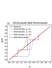
The mapping functions of the WENO-X schemes presented in Table 1 and those of the corresponding MOP-WENO-X schemes are shown in Fig. 1. We can find that, for the mapping functions of the MOP-WENO-X schemes: (1) the monotonicity over the whole domain $(0,1)$ is maintained; (2) the differentiability is reduced and limited to the neighborhood of the optimal weights $d_{s}$ ; (3) the OP property is obtained. We summarize these properties as follows.

Theorem 2

Let $\overline{\Omega}_{i}=\Big{\{}\omega\in\Omega_{i}\cap\omega\neq\partial\Omega_{i}\Big{\}},i=0,1,\cdots,r-1$ . The mapping function $\big{(}g^{\mathrm{MOP-X}}\big{)}_{s}(\omega)$ obtained from Althorithm 1 satisfies the following properties:

C1. for $\forall\omega\in\overline{\Omega}_{i},i=0,1,\cdots,r-1$ , $\big{(}g^{\mathrm{MOP-X}}\big{)}^{\prime}_{s}(\omega)\geq 0$ ;

C2. for $\forall\omega\in\Omega$ , $0\leq\big{(}g^{\mathrm{MOP-X}}\big{)}_{s}(\omega)\leq 1$ ;

C3. for $\forall s\in\Big{\{}0,1,\cdots,r-1\Big{\}}$ , $\widetilde{d}_{s}\in\Omega_{s}$ , and $\big{(}g^{\mathrm{MOP-X}}\big{)}_{s}(\widetilde{d}_{s})=\widetilde{d}_{s},\big{(}g^{\mathrm{MOP-X}}\big{)}^{\prime}_{s}(\widetilde{d}_{s})=\cdots=\big{(}g^{\mathrm{MOP-X}}\big{)}^{(n_{\mathrm{X}})}_{s}(\widetilde{d}_{s})=0$ where $n_{\mathrm{X}}$ is given in Table 1;

C4. $\big{(}g^{\mathrm{MOP-X}}\big{)}_{s}(0)=0,\big{(}g^{\mathrm{MOP-X}}\big{)}_{s}(1)=1,\big{(}g^{\mathrm{MOP-X}}\big{)}^{\prime}_{s}(0)=\big{(}g^{\mathrm{X}}\big{)}^{\prime}_{s}(0),\big{(}g^{\mathrm{MOP-X}}\big{)}^{\prime}_{s}(1)=\big{(}g^{\mathrm{X}}\big{)}^{\prime}_{s}(1)$ ;

C5. for $\forall m,n\in\Big{\{}0,\cdots,r-1\Big{\}}$ , if $\omega_{m}>\omega_{n}$ , then $\big{(}g^{\mathrm{MOP-X}}\big{)}_{m}(\omega_{m})\geq\big{(}g^{\mathrm{MOP-X}}\big{)}_{n}(\omega_{n})$ , and if $\omega_{m}=\omega_{n}$ , then $\big{(}g^{\mathrm{MOP-X}}\big{)}_{m}(\omega_{m})=\big{(}g^{\mathrm{MOP-X}}\big{)}_{n}(\omega_{n})$ .

Refer to caption — Fig. 1: Comparison for the mapping functions for WENO-X (shown in Table 1) and MOP-WENO-X.

3.4 Convergence properties

According to Theorem 2, we get the convergence properties for the $(2r-1)$ th-order MOP-WENO-X schemes as given in Theorem 3. The proof is almost identical to that of the corresponding WENO-X schemes in the references presented in Table 1.

Theorem 3

The requirements for the $(2r-1)$ th-order MOP-WENO-X schemes to achieve the optimal order of accuracy are identical to that of the corresponding $(2r-1)$ th-order WENO-X schemes.

For the integrity of this paper and the benefit of the reader, we concisely express the following Corollaries of Theorem 3.

Corollary 1

If $n$ mapping is used in the $(2r-1)$ th-order MOP-WENO-M scheme, then for different values of $n_{\mathrm{cp}}$ , the weights $\omega_{s}^{\mathrm{MOP-M}}$ in the $(2r-1)$ th-order MOP-WENO-M scheme satisfy

\omega_{s}^{\mathrm{MOP-M}}-d_{s}=O\Big{(}(\Delta x)^{3^{n}\times(r-1-n_{\mathrm{cp}})}\Big{)},\quad r=2,3,\cdots,9,\quad n_{\mathrm{cp}}=0,1,\cdots,r-1,

and the rate of convergence is

r_{\mathrm{c}}=\left\{\begin{array}[]{ll}2r-1,&\mathrm{if}\quad n_{\mathrm{cp}}=0,\cdots,\Bigg{\lfloor}\dfrac{3^{n}-1}{3^{n}}r-1\Bigg{\rfloor},\\ (3^{n}+1)(r-1)-3^{n}\times n_{\mathrm{cp}},&\mathrm{if}\quad n_{\mathrm{cp}}=\Bigg{\lfloor}\dfrac{3^{n}-1}{3^{n}}r-1\Bigg{\rfloor}+1,\cdots,r-1.\end{array}\right.

where $\lfloor x\rfloor$ is a floor function of $x$ .

Proof. The proof is almost identical to that of Lemma 6 in [16]. $\hfill\square$

Corollary 2

When $n_{\mathrm{cp}}=1$ , the $(2r-1)$ th-order MOP-WENO-IM( $k,A$ ) schemes can achieve the optimal order of accuracy if the mapping function $\big{(}g^{\mathrm{MOP-IM}}\big{)}_{s}(\omega)$ is applied to the original weights in the $(2r-1)$ th-order WENO-JS schemes with requirement of $k\geq 2$ (except for the case $r=2$ ).

Proof. The proof is almost identical to that of Theorem 2 in [4]. $\hfill\square$

Corollary 3

The $(2r-1)$ th-order MOP-WENO-PM $k$ schemes can achieve the optimal order of accuracy if the mapping function $\big{(}g^{\mathrm{MOP-PM}}\big{)}_{s}(\omega)$ is applied to the original weights in the $(2r-1)$ th-order WENO-JS schemes with specific requirements for $k$ in following different cases: (I) Require $k\geq 1$ for $n_{\mathrm{cp}}=0$ ; (II) Require $k\geq 1$ for $n_{\mathrm{cp}}=1$ ; (III) Require $k\geq 3$ for $n_{\mathrm{cp}}=2$ .

Proof. The proof is almost identical to that of Proposition 1 in [3]. $\hfill\square$

Corollary 4

The $(2r-1)$ th-order MOP-WENO-RM( $mn0$ ) schemes can recover the optimal order of accuracy if the mapping function $\big{(}g^{\mathrm{MOP-RM}}\big{)}_{s}(\omega)$ is applied to the original weights in the $(2r-1)$ th-order WENO-JS schemes with requirement of $n\geq\frac{1+n_{\mathrm{cp}}}{r-1-n_{\mathrm{cp}}}$ for different values of $n_{\mathrm{cp}}$ with $1\leq n_{\mathrm{cp}}<r-1$ .

Proof. The proof is almost identical to that of Theorem 3 in [29]. $\hfill\square$

Corollary 5

Let $\lceil x\rceil$ be a ceiling function of $x$ , for $n_{\mathrm{cp}}<r-1$ , the $(2r-1)$ th-order MOP-WENO-MAIM $1$ schemes can achieve the optimal order of accuracy if the mapping function $(g^{\mathrm{MOP-MAIM}1})_{s}(\omega)$ is applied to the original weights in the $(2r-1)$ th-order WENO-JS schemes with requirement of $k\geq k^{\mathrm{MAIM}}$ , where

k^{\mathrm{MAIM}}=\Bigg{\lceil}\dfrac{r}{r-1-n_{\mathrm{cp}}}-2\Bigg{\rceil}+\dfrac{1+\Big{(}-1\Big{)}^{\Bigg{\lceil}\dfrac{r}{r-1-n_{\mathrm{cp}}}-2\Bigg{\rceil}}}{2}.

Proof. The proof is almost identical to that of Theorem 2 in [16]. $\hfill\square$

Corollary 6

For $n_{\mathrm{cp}}<r-1$ , the $(2r-1)$ th-order MOP-WENO-ACM schemes can achieve the optimal order of accuracy if the mapping function $(g^{\mathrm{MOP-ACM}})_{s}(\omega)$ is applied to the original weights in the $(2r-1)$ th-order WENO-JS schemes.

Proof. The proof is almost identical to that of Theorem 2 in [17]. $\hfill\square$

Corollary 7

When $\mathrm{CFS}_{s}\ll\widetilde{d}_{0}$ , for $n_{\mathrm{cp}}<r-1$ , the $(2r-1)$ th-order MOP-WENO-ACM $k$ schemes can achieve the optimal order of accuracy if the mapping function $(g^{\mathrm{MOP-ACM}k})_{s}(\omega)$ is applied to the original weights in the $(2r-1)$ th-order WENO-JS schemes.

Proof. The proof is almost identical to that of Theorem 2 in [18]. $\hfill\square$

4 Numerical results

In this section, we compare the numerical performances of the MOP-WENO-X schemes with the corresponding existing mapped WENO-X schemes shown in Table 1, as well as the classic WENO-JS scheme. As the performances of the WENO-ACM scheme and the MOP-WENO-ACM scheme are almost identical to those of the MIP-WENO-ACM $k$ scheme and the MOP-WENO-ACM $k$ scheme respectively, we do not present the solutions of the WENO-ACM scheme and the MOP-WENO-ACM scheme below for simplicity. Typical one-dimensional linear advection equation and two-dimensional Euler equations, with different initial conditions, are used to test the considered schemes. The presentation of these numerical tests in this section starts with the accuracy test of one-dimensional linear advection equation with four different initial conditions, followed by the long output time simulations of it with two different initial conditions including discontinuities, and finishes with two-dimensional simulations on the shock-vortex interaction and the 2D Riemann problem. In all calculations below, $\epsilon$ is taken to be $10^{-40}$ for all schemes following the recommendations in [11, 4].

In the following numerical tests, the ODEs resulting from the semi-discretized PDEs are marched in time using the following explicit, third-order, strong stability preserving (SSP) Runge-Kutta method [26, 5, 6]

\begin{array}[]{l}\begin{aligned} &\overrightarrow{U}^{*}=\overrightarrow{U}^{n}+\Delta t\mathcal{L}(\overrightarrow{U}^{n}),\\ &\overrightarrow{U}^{**}=\dfrac{3}{4}\overrightarrow{U}^{n}+\dfrac{1}{4}\overrightarrow{U}^{*}+\dfrac{1}{4}\Delta t\mathcal{L}(\overrightarrow{U}^{*}),\\ &\overrightarrow{U}^{n+1}=\dfrac{1}{3}\overrightarrow{U}^{n}+\dfrac{2}{3}\overrightarrow{U}^{**}+\dfrac{2}{3}\Delta t\mathcal{L}(\overrightarrow{U}^{**}),\end{aligned}\end{array}

where $\overrightarrow{U}^{*}$ , $\overrightarrow{U}^{**}$ are the intermediate stages, $\overrightarrow{U}^{n}$ is the value of $\overrightarrow{U}$ at time level $t^{n}=n\Delta t$ , and $\Delta t$ is the time step satisfying some proper CFL condition. The spatial operator $\mathcal{L}$ is defined as in Eq.(3), and the WENO reconstructions will be applied to obtain it.

4.1 Accuracy test

In this subsection, we solve the following one-dimensional linear advection equation

\dfrac{\partial u}{\partial t}+\dfrac{\partial u}{\partial x}=0,\quad-1\leq x\leq 1,

(37)

with different initial conditions to test the accuracy of the considered WENO schemes. In all accuracy tests, the $L_{1},L_{2},L_{\infty}$ norms of the error are given as

\displaystyle\begin{array}[]{l}L_{1}=h\cdot\displaystyle\sum\limits_{j}\big{\lvert}u_{j}^{\mathrm{exact}}-(u_{h})_{j}\big{\rvert},\\ L_{2}=\sqrt{h\cdot\displaystyle\sum\limits_{j}(u_{j}^{\mathrm{exact}}-(u_{h})_{j})^{2}},\\ L_{\infty}=\displaystyle\max_{j}\big{\lvert}u_{j}^{\mathrm{exact}}-(u_{h})_{j}\big{\rvert},\end{array}

where $h=\Delta x$ is the uniform spatial step size, $(u_{h})_{j}$ is the numerical solution and $u_{j}^{\mathrm{exact}}$ is the exact solution.

Example 1

We calculate Eq.(37) with the periodic boundary condition using the following initial condition [4]

u(x,0)=\sin(\pi x).

(38)

It is trivial to verify that although the initial condition in Eq.(38) has two first-order critical points, their first and third derivatives vanish simultaneously. The CFL number is taken to be $(\Delta x)^{2/3}$ to prevent the convergence rates of error from being influenced by time advancement. The calculation is run until a time of $t=2.0$ .

In Table 2, we show the $L_{1},L_{2},L_{\infty}$ errors and corresponding convergence orders of various considered WENO schemes. The results of the three rows are $L_{1}$ -, $L_{2}$ - and $L_{\infty}$ - norm errors and convergence orders (in brackets) in turn (similarly hereinafter). Unsurprisingly, the MOP-WENO-X schemes and the corresponding WENO-X schemes provide more accurate results than the WENO-JS scheme do in general. Naturally and as expected, all the considered schemes have gained the fifth-order convergence rate of accuracy. It can be found that the results of the MOP-WENO-X schemes are identical to those of the corresponding WENO-X schemes for all grid numbers except $N=10$ . As discussed in [18], the cause of the accuracy loss for the computing cases of all MOP-WENO-X schemes with $N=10$ is that the mapping functions of the MOP-WENO-X schemes have narrower optimal weight intervals (standing for the intervals about $\omega=d_{s}$ over which the mapping process attempts to use the corresponding optimal weights, see [16, 17]) than the corresponding WENO-X schemes.

Table 2: Convergence properties of considered schemes solving

u_{t}+u_{x}=0

with initial condition

u(x,0)=\sin(\pi x)

$N$	10	20	40	80	160	320
WENO-JS	6.18628e-02(-)	2.96529e-03(4.3821)	9.27609e-05(4.9985)	2.89265e-06(5.0031)	9.03392e-08(5.0009)	2.82330e-09(4.9999)
	4.72306e-02(-)	2.42673e-03(4.2826)	7.64332e-05(4.9887)	2.33581e-06(5.0322)	7.19259e-08(5.0213)	2.23105e-09(5.0107)
	4.87580e-02(-)	2.57899e-03(4.2408)	9.05453e-05(4.8320)	2.90709e-06(4.9610)	8.85753e-08(5.0365)	2.72458e-09(5.0228)
WENO-M	2.01781e-02(-)	5.18291e-04(5.2829)	1.59422e-05(5.0228)	4.98914e-07(4.9979)	1.56021e-08(4.9990)	4.99356e-10(4.9977)
	1.55809e-02(-)	4.06148e-04(5.2616)	1.25236e-05(5.0193)	3.91875e-07(4.9981)	1.22541e-08(4.9991)	3.83568e-10(4.9976)
	1.47767e-02(-)	3.94913e-04(5.2256)	1.24993e-05(4.9816)	3.91808e-07(4.9956)	1.22538e-08(4.9988)	3.83541e-10(4.9977)
MOP-WENO-M	3.64427e-02(-)	5.18291e-04(6.1357)	1.59422e-05(5.0228)	4.98914e-07(4.9979)	1.56021e-08(4.9990)	4.88356e-10(4.9977)
	2.95270e-02(-)	4.06148e-04(6.1839)	1.25236e-05(5.0193)	3.91875e-07(4.9981)	1.22541e-08(4.9991)	3.83568e-10(4.9976)
	2.81876e-02(-)	3.94913e-04(6.1574)	1.24993e-05(4.9816)	3.91808e-07(4.9956)	1.22538e-08(4.9988)	3.83541e-10(4.9977)
WENO-IM(2,0.1)	1.58051e-02(-)	5.04401e-04(4.9697)	1.59160e-05(4.9860)	4.98863e-07(4.9957)	1.56020e-08(4.9988)	4.88355e-10(4.9977)
	1.23553e-02(-)	3.96236e-04(4.9626)	1.25033e-05(4.9860)	3.91836e-07(4.9959)	1.22541e-08(4.9989)	3.83568e-10(4.9976)
	1.19178e-02(-)	3.94458e-04(4.9171)	1.24963e-05(4.9803)	3.91797e-07(4.9953)	1.22538e-08(4.9988)	3.83547e-10(4.9977)
MOP-WENO-IM(2,0.1)	3.35513e-02(-)	5.04401e-04(6.0557)	1.59160e-05(4.9860)	4.98863e-07(4.9957)	1.56020e-08(4.9988)	4.88355e-10(4.9977)
	2.75968e-02(-)	3.96236e-04(6.1220)	1.25033e-05(4.9860)	3.91836e-07(4.9959)	1.22541e-08(4.9989)	3.83568e-10(4.9976)
	2.71898e-02(-)	3.94458e-04(6.1071)	1.24963e-05(4.9803)	3.91797e-07(4.9953)	1.22538e-08(4.9988)	3.83547e-10(4.9977)
WENO-PM6	1.74869e-02(-)	5.02923e-04(5.1198)	1.59130e-05(4.9821)	4.98858e-07(4.9954)	1.56020e-08(4.9988)	4.88355e-10(4.9977)
	1.35606e-02(-)	3.95215e-04(5.1006)	1.25010e-05(4.9825)	3.91831e-07(4.9957)	1.22541e-08(4.9989)	3.83568e-10(4.9976)
	1.27577e-02(-)	3.94515e-04(5.0151)	1.24960e-05(4.9805)	3.91795e-07(4.9952)	1.22538e-08(4.9988)	3.83543e-10(4.9977)
MOP-WENO-PM6	3.54584e-02(-)	5.02923e-04(6.1396)	1.59130e-05(4.9821)	4.98858e-07(4.9954)	1.56020e-08(4.9988)	4.88355e-10(4.9977)
	2.88246e-02(-)	3.95215e-04(6.1885)	1.25010e-05(4.9825)	3.91831e-07(4.9957)	1.22541e-08(4.9989)	3.83568e-10(4.9976)
	2.76902e-02(-)	3.94515e-04(6.1332)	1.24960e-05(4.9805)	3.91795e-07(4.9952)	1.22538e-08(4.9988)	3.83543e-10(4.9977)
WENO-PPM5	1.73978e-02(-)	5.03464e-04(5.1109)	1.59131e-05(4.9836)	4.98858e-07(4.9954)	1.56020e-08(4.9988)	4.88356e-10(4.9977)
	1.34998e-02(-)	3.95644e-04(5.0926)	1.25011e-05(4.9841)	3.91831e-07(4.9957)	1.22541e-08(4.9989)	3.83568e-10(4.9976)
	1.27018e-02(-)	3.94865e-04(5.0075)	1.24961e-05(4.9818)	3.91795e-07(4.9952)	1.22538e-08(4.9988)	3.83528e-10(4.9978)
MOP-WENO-PPM5	3.49872e-02(-)	5.03464e-04(6.1188)	1.59131e-05(4.9836)	4.98858e-07(4.9954)	1.56020e-08(4.9988)	4.88356e-10(4.9977)
	2.85173e-02(-)	3.95644e-04(6.1715)	1.25011e-05(4.9841)	3.91831e-07(4.9957)	1.22541e-08(4.9989)	3.83568e-10(4.9976)
	2.75955e-02(-)	3.94865e-04(6.1269)	1.24961e-05(4.9818)	3.91795e-07(4.9952)	1.22538e-08(4.9988)	3.83528e-10(4.9978)
WENO-RM(260)	1.52661e-02(-)	5.02845e-04(4.9241)	1.59130e-05(4.9818)	4.98858e-07(4.9954)	1.56020e-08(4.9988)	4.88355e-10(4.9977)
	1.19792e-02(-)	3.95138e-04(4.9220)	1.25010e-05(4.9822)	3.91831e-07(4.9957)	1.22541e-08(4.9989)	3.83568e-10(4.9976)
	1.17698e-02(-)	3.94406e-04(4.8993)	1.24960e-05(4.9801)	3.91795e-07(4.9952)	1.22538e-08(4.9988)	3.83543e-10(4.9977)
MOP-WENO-RM(260)	3.29243e-02(-)	5.02845e-04(6.0329)	1.59130e-05(4.9818)	4.98858e-07(4.9954)	1.56020e-08(4.9988)	4.88355e-10(4.9977)
	2.73131e-02(-)	3.95138e-04(6.1111)	1.25010e-05(4.9822)	3.91831e-07(4.9957)	1.22541e-08(4.9989)	3.83568e-10(4.9976)
	2.73015e-02(-)	3.94406e-04(6.1132)	1.24960e-05(4.9801)	3.91795e-07(4.9952)	1.22538e-08(4.9988)	3.83543e-10(4.9977)
WENO-MAIM1	6.13264e-02(-)	5.08205e-04(6.9150)	1.59130e-05(4.9971)	4.98858e-07(4.9954)	1.56020e-08(4.9988)	4.88355e-10(4.9977)
	4.81375e-02(-)	4.26155e-04(6.8196)	1.25010e-05(5.0913)	3.91831e-07(4.9957)	1.22541e-08(4.9989)	3.83568e-10(4.9976)
	4.86913e-02(-)	5.03701e-04(6.5950)	1.24960e-05(5.3330)	3.91795e-07(4.9952)	1.22538e-08(4.9988)	3.83543e-10(4.9977)
MOP-WENO-MAIM1	6.63923e-02(-)	5.08205e-04(7.0295)	1.59130e-05(4.9971)	4.98858e-07(4.9954)	1.56020e-08(4.9988)	4.88355e-10(4.9977)
	5.17462e-02(-)	4.26155e-04(6.9239)	1.25010e-05(5.0913)	3.91831e-07(4.9957)	1.22541e-08(4.9989)	3.83568e-10(4.9976)
	5.19799e-02(-)	5.03701e-04(6.6892)	1.24960e-05(5.3330)	3.91795e-07(4.9952)	1.22538e-08(4.9988)	3.83543e-10(4.9977)
MIP-WENO-ACM $k$	1.52184e-02(-)	5.02844e-04(4.9196)	1.59130e-05(4.9818)	4.98858e-07(4.9954)	1.56020e-08(4.9988)	4.88355e-10(4.9977)
	1.19442e-02(-)	3.95138e-04(4.9178)	1.25010e-05(4.9822)	3.91831e-07(4.9957)	1.22541e-08(4.9989)	3.83568e-10(4.9976)
	1.17569e-02(-)	3.94406e-04(4.8977)	1.24960e-05(4.9801)	3.91795e-07(4.9952)	1.22538e-08(4.9988)	3.83543e-10(4.9977)
MOP-WENO-ACM $k$	3.29609e-02(-)	5.02844e-04(6.0345)	1.59130e-05(4.9818)	4.98858e-07(4.9954)	1.56020e-08(4.9988)	4.88355e-10(4.9977)
	2.72363e-02(-)	3.95138e-04(6.1070)	1.25010e-05(4.9822)	3.91831e-07(4.9957)	1.22541e-08(4.9989)	3.83568e-10(4.9976)
	2.70295e-02(-)	3.94406e-04(6.0987)	1.24960e-05(4.9801)	3.91795e-07(4.9952)	1.22538e-08(4.9988)	3.83543e-10(4.9977)

Example 2

We calculate Eq.(37) with the periodic boundary condition using the following initial condition [11]

u(x,0)=\sin\bigg{(}\pi x-\dfrac{\sin(\pi x)}{\pi}\bigg{)},

(39)

This particular initial condition has two first-order critical points, which both have a non-vanishing third derivative. Again, the CFL number is set to be $(\Delta x)^{2/3}$ and the calculation is run until a time of $t=2.0$ .

Table 3 compares the $L_{1},L_{2},L_{\infty}$ errors and corresponding convergence orders obtained from the considered schemes. It is evident that the WENO-X schemes and the corresponding MOP-WENO-X schemes can achieve the optimal convergence orders. Unsurprisingly, the WENO-JS scheme gives less accurate results than the other schemes, and its $L_{\infty}$ convergence order decreases by almost 2 orders leading to the noticeable drops of the $L_{1}$ and $L_{2}$ convergence orders. It is noteworthy that when the grid number is too small, like $N\leq 40$ , in terms of accuracy, the MOP-WENO-X schemes provide less accurate results than those of the corresponding WENO-X schemes. As mentioned in Example 1, the cause of this kind of accuracy loss is that the mapping functions of the MOP-WENO-X schemes have narrower optimal weight intervals than the corresponding WENO-X schemes, and this issue can surely be addressed by increasing the grid number. Therefore, as expected, the MOP-WENO-X schemes show equally accurate numerical solutions like those of the corresponding WENO-X schemes when the grid number $N\geq 80$ .

Table 3: Convergence properties of considered schemes solving

u_{t}+u_{x}=0

with initial condition

u(x,0)=\sin(\pi x-\sin(\pi x)/\pi)

$N$	10	20	40	80	160	320
WENO-JS	1.24488e-01(-)	1.01260e-02(3.6199)	7.22169e-04(3.8096)	3.42286e-05(4.3991)	1.58510e-06(4.4326)	7.95517e-08(4.3165)
	1.09463e-01(-)	8.72198e-03(3.6496)	6.76133e-04(3.6893)	3.63761e-05(4.2162)	2.29598e-06(3.9858)	1.68304e-07(3.7700)
	1.24471e-01(-)	1.43499e-02(3.1167)	1.09663e-03(3.7099)	9.02485e-05(3.6030)	8.24022e-06(3.4531)	8.31702e-07(3.3085)
WENO-M	7.53259e-02(-)	3.70838e-03(4.3443)	1.45082e-04(4.6758)	4.80253e-06(4.9169)	1.52120e-07(4.9805)	4.77083e-09(4.9948)
	6.39017e-02(-)	3.36224e-03(4.2484)	1.39007e-04(4.5962)	4.52646e-06(4.9406)	1.42463e-07(4.9897)	4.45822e-09(4.9980)
	7.49250e-02(-)	5.43666e-03(3.7847)	2.18799e-04(4.6350)	6.81451e-06(5.0049)	2.14545e-07(4.9893)	6.71080e-09(4.9987)
MOP-WENO-M	9.41832e-02(-)	6.59540e-03(3.8359)	2.60456e-04(4.6623)	4.80253e-06(5.7611)	1.52120e-07(4.9805)	4.77083e-09(4.9948)
	8.03446e-02(-)	6.37937e-03(3.6547)	2.50868e-04(4.6684)	4.52646e-06(5.7924)	1.42463e-07(4.9897)	4.45822e-09(4.9980)
	9.78919e-02(-)	8.97094e-03(3.4479)	4.10480e-04(4.4499)	6.81451e-06(5.9126)	2.14545e-07(4.9893)	6.71080e-09(4.9987)
WENO-IM(2,0.1)	8.38131e-02(-)	4.30725e-03(4.2823)	1.51327e-04(4.8310)	4.85592e-06(4.9618)	1.52659e-07(4.9914)	4.77654e-09(4.9982)
	6.71285e-02(-)	3.93700e-03(4.0918)	1.41737e-04(4.7958)	4.53602e-06(4.9656)	1.42479e-07(4.9926)	4.45805e-09(4.9982)
	7.62798e-02(-)	5.84039e-03(3.7072)	2.10531e-04(4.7940)	6.82606e-06(4.9468)	2.14534e-07(4.9918)	6.71079e-09(4.9986)
MOP-WENO-IM(2,0.1)	8.49795e-02(-)	7.01287e-03(3.5990)	2.59767e-04(4.7547)	4.85592e-06(5.7413)	1.52659e-07(4.9914)	4.77654e-09(4.9982)
	7.29388e-02(-)	6.80019e-03(3.4230)	2.51121e-04(4.7591)	4.53602e-06(5.7908)	1.42479e-07(4.9926)	4.45805e-09(4.9982)
	9.47429e-02(-)	9.96943e-03(3.2484)	4.01785e-04(4.6330)	6.82606e-06(5.8792)	2.14534e-07(4.9918)	6.71079e-09(4.9986)
WENO-PM6	9.51313e-02(-)	4.82173e-03(4.3023)	1.55428e-04(4.9552)	4.87327e-06(4.9952)	1.52750e-07(4.9956)	4.77729e-09(4.9988)
	7.83600e-02(-)	4.29510e-03(4.1894)	1.43841e-04(4.9001)	4.54036e-06(4.9855)	1.42488e-07(4.9939)	4.45807e-09(4.9983)
	9.32356e-02(-)	5.91037e-03(3.9796)	2.09540e-04(4.8180)	6.83270e-06(4.9386)	2.14532e-07(4.9932)	6.71079e-09(4.9986)
MOP-WENO-PM6	1.00298e-01(-)	5.84504e-03(4.1009)	2.51725e-04(4.5373)	4.87327e-06(5.6908)	1.52750e-07(4.9956)	4.77729e-09(4.9988)
	8.49034e-02(-)	5.80703e-03(3.8699)	2.40678e-04(4.5926)	4.54036e-06(5.7282)	1.42488e-07(4.9939)	4.45807e-09(4.9983)
	9.88357e-02(-)	9.01779e-03(3.4542)	3.66822e-04(4.6196)	6.83270e-06(5.7465)	2.14532e-07(4.9932)	6.71079e-09(4.9986)
WENO-PPM5	9.22982e-02(-)	4.68376e-03(4.3006)	1.55745e-04(4.9104)	4.88795e-06(4.9938)	1.52852e-07(4.9990)	4.77759e-09(4.9997)
	7.46925e-02(-)	4.18882e-03(4.1563)	1.44018e-04(4.8622)	4.54528e-06(4.9857)	1.42506e-07(4.9953)	4.45812e-09(4.9984)
	8.46229e-02(-)	5.92748e-03(3.8356)	2.09420e-04(4.8229)	6.83617e-06(4.9371)	2.14527e-07(4.9940)	6.71080e-09(4.9985)
MOP-WENO-PPM5	9.50369e-02(-)	6.27179e-03(3.9215)	2.52600e-04(4.6340)	4.88795e-06(5.6915)	1.52852e-07(4.9990)	4.77759e-09(4.9997)
	8.08190e-02(-)	6.11267e-03(3.7248)	2.41656e-04(4.6608)	4.54528e-06(5.7324)	1.42506e-07(4.9953)	4.45812e-09(4.9984)
	9.65522e-02(-)	8.98120e-03(3.4263)	3.69338e-04(4.6039)	6.83617e-06(5.7556)	2.14527e-07(4.9940)	6.71080e-09(4.9985)
WENO-RM(260)	8.24328e-02(-)	4.37642e-03(4.2354)	1.52200e-04(4.8457)	4.86434e-06(4.9676)	1.52735e-07(4.9931)	4.77728e-09(4.9987)
	6.64590e-02(-)	4.00547e-03(4.0524)	1.42162e-04(4.8164)	4.53769e-06(4.9694)	1.42486e-07(4.9931)	4.45807e-09(4.9983)
	7.64206e-02(-)	5.88375e-03(3.6992)	2.09889e-04(4.8090)	6.83016e-06(4.9416)	2.14533e-07(4.9926)	6.71079e-09(4.9986)
MOP-WENO-RM(260)	8.96509e-02(-)	6.87612e-03(3.7047)	2.59418e-04(4.7282)	4.86434e-06(5.7369)	1.52735e-07(4.9931)	4.77728e-09(4.9987)
	7.51169e-02(-)	6.65488e-03(3.4967)	2.51194e-04(4.7275)	4.53769e-06(5.7907)	1.42486e-07(4.9931)	4.45807e-09(4.9983)
	9.20962e-02(-)	9.75043e-03(3.2396)	4.03065e-04(4.5964)	6.83016e-06(5.8829)	2.14533e-07(4.9926)	6.71079e-09(4.9986)
WENO-MAIM1	1.24659e-01(-)	8.07923e-03(3.9476)	3.32483e-04(4.6029)	1.01162e-05(5.0385)	1.52910e-07(6.0478)	4.77728e-09(5.0003)
	1.14152e-01(-)	7.08117e-03(4.0108)	3.36264e-04(4.3963)	1.49724e-05(4.4892)	1.42515e-07(6.7150)	4.45807e-09(4.9986)
	1.40438e-01(-)	1.03772e-02(3.7584)	6.62891e-04(3.9685)	4.48554e-05(3.8854)	2.14522e-07(7.7080)	6.71079e-09(4.9985)
MOP-WENO-MAIM1	1.27999e-01(-)	7.62753e-03(4.0688)	3.37132e-04(4.4998)	1.01162e-05(5.0586)	1.52910e-07(6.0478)	4.77728e-09(5.0003)
	1.12692e-01(-)	6.93240e-03(4.0229)	3.36497e-04(4.3647)	1.49724e-05(4.4902)	1.42515e-07(6.7150)	4.45807e-09(4.9986)
	1.31113e-01(-)	1.27480e-02(3.3625)	6.40953e-04(4.3139)	4.48554e-05(3.8369)	2.14522e-07(7.7080)	6.71079e-09(4.9985)
MIP-WENO-ACM $k$	8.75629e-02(-)	4.39527e-03(4.3163)	1.52219e-04(4.8517)	4.86436e-06(4.9678)	1.52735e-07(4.9931)	4.77728e-09(4.9987)
	6.98131e-02(-)	4.02909e-03(4.1150)	1.42172e-04(4.8247)	4.53770e-06(4.9695)	1.42486e-07(4.9931)	4.45807e-09(4.9983)
	7.91292e-02(-)	5.89045e-03(3.7478)	2.09893e-04(4.8107)	6.83017e-06(4.9416)	2.14533e-07(4.9926)	6.71079e-09(4.9986)
MOP-WENO-ACM $k$	9.08634e-02(-)	7.09246e-03(3.6793)	2.59429e-04(4.7729)	4.86436e-06(5.7369)	1.52735e-07(4.9931)	4.77728e-09(4.9987)
	7.58160e-02(-)	6.88532e-03(3.4609)	2.51208e-04(4.7766)	4.53770e-06(5.7908)	1.42486e-07(4.9931)	4.45807e-09(4.9983)
	9.29135e-02(-)	1.01479e-02(3.1947)	4.03069e-04(4.6540)	6.83017e-06(5.8830)	2.14533e-07(4.9926)	6.71079e-09(4.9986)

Example 3

We calculate Eq.(37) using the following initial condition [3]

u(x,0)=\sin^{9}(\pi x),

(40)

with the periodic boundary condition. It is trivial to verify that this initial condition has high-order critical points. We also set the CFL number to be $(\Delta x)^{2/3}$ .

Table 4 shows the $L_{1},L_{2},L_{\infty}$ errors of the considered WENO schemes at several output times with a uniform mesh size of $\Delta x=1/200$ . In order to measure the dissipations of the schemes, as the authors did in [18], we give the corresponding increased errors (in percentage) compared to the MIP-WENO-ACM $k$ scheme which gives solutions with very low dissipations. Taking the $L_{1}$ -norm error as an example, let $L_{1}^{*}(t)$ and $L_{1}^{\mathrm{Y}}(t)$ the $L_{1}$ -norm errors of the MIP-WENO-ACM $k$ scheme and the compared scheme, the increased errors at output time $t$ is computed by $\frac{L_{1}^{\mathrm{Y}}(t)-L_{1}^{*}(t)}{L_{1}^{*}(t)}\times 100\%$ . From Table 4, we can observe that: (1) the WENO-JS scheme shows the largest increased errors for no matter short or long output times; (2) at short output times, like $t\leq 100$ , the solutions computed by the WENO-M scheme are closer to those of the MIP-WENO-ACM $k$ scheme, leading to smaller increased errors, than the corresponding MOP-WENO-M scheme; (3) however, when the output time is larger, like $t\geq 200$ , the solutions computed by the MOP-WENO-M scheme, whose increased errors do not get larger but evidently decrease, are closer to those of the MIP-WENO-ACM $k$ scheme than the corresponding WENO-M scheme whose errors increase dramatically leading to significantly larger increased errors; (4) although the errors of the MOP-WENO-X schemes except the MOP-WENO-M scheme are not as small as those of the corresponding WENO-X schemes, these errors can maintain a considerable level leading to acceptable increased errors that are much lower than those of the WENO-JS and WENO-M schemes.

Actually, as mentioned in Example 1 and Example 2, the cause of the slight accuracy loss discussed above is that the mapping function of the MOP-WENO-X scheme has narrower optimal weight intervals than the corresponding WENO-X schemes, and one can easily overcome this drawback by increasing the grid number. To demonstrate this, we calculate this problem using the same schemes at the same output times with a larger grid number of $N=800$ . The results are shown in Table 5, and we can see that: (1) the errors of the MOP-WENO-X schemes get closer to those of the MIP-WENO-ACM $k$ scheme when the grid number increases from $N=200$ to $N=800$ , resulting in the significant decrease of the increased errors, and in different words, the errors of the MOP-WENO-X schemes and the MIP-WENO-ACM $k$ scheme are so close that one can ignore their differences; (2) although the errors of the WENO-JS and WENO-M schemes get smaller when the grid number increases from $N=200$ to $N=800$ , their increased errors become very very large; (3) naturally, the increased errors of the MOP-WENO-X schemes are extremely smaller than those of the WENO-JS and WENO-M schemes. Actually, it is an important advantage of the MOP-WENO-X schemes that can maintain comparably high resolution for long output times. In the next subsection we will make a further discussion for this.

In Fig. 2 and Fig. 3, we plot the solutions computed by various schemes at output time $t=1000$ with the grid number of $N=200$ and $N=800$ , respectively. For $N=200$ , Fig. 2 shows that: (1) the MOP-WENO-M scheme provides the result with far higher resolution than the corresponding WENO-M scheme which gives result with slightly better resolution than the lowest one computed by the WENO-JS scheme; (2) the result of the MOP-WENO-MAIM1 scheme is very close to that of its corresponding WENO-MAIM1 scheme; (3) the results of the other MOP-WENO-X schemes show far better resolutions than the WENO-M and WENO-JS schemes, although they give results with very slightly lower resolutions than their corresponding WENO-X schemes because of the narrower optimal weight intervals. Actually, we can amend this minor issue by using a larger grid number. Consequently, for $N=800$ , it can be seen from Fig. 3 that: (1) all the MOP-WENO-X schemes produce results very close to those of their corresponding mapped WENO-X schemes with extremely high resolutions except the case of X = M; (2) the MOP-WENO-M scheme also produces result with very high resolution, while the resolutions of the results from the WENO-M and WENO-JS schemes are much lower.

Table 4: Performance of various considered schemes solving

u_{t}+u_{x}=0

with

u(x,0)=\sin^{9}(\pi x),\Delta x=1/200

Scheme	$t=10$	$t=100$	$t=200$	$t=500$	$t=1000$
WENO-JS	3.86931e-04(359.06%)	5.42288e-03(548.87%)	2.35657e-02(1323.42%)	1.55650e-01(3832.05%)	2.91359e-01(3920.28%)
	3.52611e-04(330.48%)	5.17716e-03(539.41%)	2.68753e-02(1580.45%)	1.46859e-01(3716.48%)	2.66692e-01(3595.71%)
	5.36940e-04(288.51%)	1.20056e-02(780.15%)	6.47820e-02(2308.66%)	2.57663e-01(3891.29%)	4.44664e-01(3556.96%)
WENO-M	8.90890e-05(5.70%)	1.29154e-03(54.54%)	5.74021e-03(246.72%)	4.89290e-02(1136.05%)	1.34933e-01(1761.86%)
	8.32089e-05(1.58%)	1.28740e-03(59.00%)	7.66721e-03(379.41%)	6.23842e-02(1521.20%)	1.46524e-01(1930.47%)
	1.38348e-04(0.10%)	3.32665e-03(143.88%)	2.37125e-02(781.65%)	1.78294e-01(2661.83%)	3.17199e-01(2508.69%)
MOP-WENO-M	1.56466e-04(85.63%)	2.88442e-03(245.13%)	5.11795e-03(209.14%)	9.09352e-03(129.72%)	1.75990e-02(142.84%)
	1.63200e-04(99.24%)	3.40815e-03(320.93%)	4.87507e-03(204.83%)	8.61108e-03(123.78%)	1.70893e-02(136.82%)
	5.08956e-04(268.26%)	1.01393e-02(643.33%)	1.02172e-02(279.89%)	1.98022e-02(206.74%)	4.01776e-02(230.43%)
WENO-IM(2, 0.1)	8.46989e-05(0.49%)	8.39425e-04(0.44%)	1.67834e-03(1.38%)	4.17514e-03(5.47%)	8.13666e-03(12.27%)
	8.20061e-05(0.12%)	8.10915e-04(0.15%)	1.60667e-03(0.46%)	3.93647e-03(2.30%)	7.71028e-03(6.85%)
	1.38220e-04(0.01%)	1.36420e-03(0.01%)	2.68977e-03(0.01%)	6.45231e-03(-0.05%)	1.21388e-02(-0.17%)
MOP-WENO-IM(2, 0.1)	1.55777e-04(84.82%)	2.74109e-03(227.98%)	4.16210e-03(151.40%)	8.37898e-03(111.67%)	1.25166e-02(72.71%)
	1.62626e-04(98.54%)	3.25705e-03(302.26%)	3.76225e-03(135.25%)	8.02344e-03(108.51%)	1.14682e-02(58.92%)
	5.08361e-04(267.83%)	9.88287e-03(624.53%)	6.81406e-03(153.35%)	1.84998e-02(186.57%)	2.02754e-02(66.75%)
WENO-PM6	8.40259e-05(-0.31%)	8.30374e-04(-0.64%)	1.63963e-03(-0.96%)	3.88864e-03(-1.76%)	7.17606e-03(-0.98%)
	8.19676e-05(0.07%)	8.09152e-04(-0.07%)	1.59697e-03(-0.15%)	3.83159e-03(-0.43%)	7.19008e-03(-0.36%)
	1.38205e-04(0.00%)	1.36410e-03(0.00%)	2.68938e-03(-0.01%)	6.45650e-03(0.01%)	1.21637e-02(0.04%)
MOP-WENO-PM6	1.53937e-04(82.63%)	2.70283e-03(223.40%)	4.07454e-03(146.11%)	8.46326e-03(113.80%)	1.54196e-02(112.77%)
	1.59169e-04(94.32%)	3.19156e-03(294.18%)	3.66635e-03(129.25%)	8.02943e-03(108.66%)	1.49590e-02(107.30%)
	4.92116e-04(256.08%)	9.52154e-03(598.04%)	6.49923e-03(141.65%)	1.83171e-02(183.74%)	3.15065e-02(159.11%)
WENO-PPM5	8.40198e-05(-0.32%)	8.30119e-04(-0.67%)	1.63931e-03(-0.98%)	3.89396e-03(-1.63%)	7.20573e-03(-0.57%)
	8.19609e-05(0.06%)	8.09118e-04(-0.07%)	1.59692e-03(-0.15%)	3.83250e-03(-0.40%)	7.19622e-03(-0.28%)
	1.38206e-04(0.00%)	1.36411e-03(0.01%)	2.68939e-03(-0.01%)	6.45658e-03(0.01%)	1.21629e-02(0.03%)
MOP-WENO-PPM5	1.53322e-04(81.90%)	2.70476e-03(223.63%)	4.17894e-03(152.42%)	8.34997e-03(110.94%)	1.21149e-02(67.17%)
	1.59164e-04(94.31%)	3.20725e-03(296.11%)	3.78313e-03(136.55%)	7.98345e-03(107.47%)	1.09845e-02(52.22%)
	4.97691e-04(260.11%)	9.71919e-03(612.53%)	6.89990e-03(156.54%)	1.83470e-02(184.20%)	1.87607e-02(54.29%)
WENO-RM(260)	8.43348e-05(0.06%)	8.35534e-04(-0.03%)	1.65314e-03(-0.15%)	3.94006e-03(-0.47%)	7.25689e-03(0.13%)
	8.19287e-05(0.02%)	8.09704e-04(0.00%)	1.59924e-03(0.00%)	3.84494e-03(-0.08%)	7.22386e-03(0.11%)
	1.38206e-04(0.00%)	1.36404e-03(0.00%)	2.68956e-03(0.00%)	6.45544e-03(0.00%)	1.21576e-02(-0.01%)
MOP-WENO-RM(260)	1.55787e-04(84.83%)	2.72147e-03(225.63%)	4.13179e-03(149.57%)	8.32505e-03(110.31%)	1.57577e-02(117.43%)
	1.62604e-04(98.51%)	3.22596e-03(298.42%)	3.73345e-03(133.44%)	7.96768e-03(107.06%)	1.53795e-02(113.12%)
	5.05390e-04(265.68%)	9.74612e-03(614.50%)	6.71615e-03(149.71%)	1.83262e-02(183.88%)	3.30552e-02(171.85%)
WENO-MAIM1	8.24623e-05(-2.17%)	8.03920e-04(-3.81%)	1.58626e-03(-4.19%)	3.77900e-03(-4.53%)	7.04287e-03(-2.82%)
	8.18028e-05(-0.13%)	8.04763e-04(-0.61%)	1.58610e-03(-0.82%)	3.79788e-03(-1.30%)	7.14409e-03(-1.00%)
	1.38215e-04(0.01%)	1.36392e-03(-0.01%)	2.68849e-03(-0.04%)	6.46356e-03(0.12%)	1.21473e-02(-0.10%)
MOP-WENO-MAIM1	9.97376e-05(18.33%)	8.16839e-04(-2.26%)	1.60912e-03(-2.81%)	6.83393e-03(72.64%)	1.24817e-02(72.23%)
	8.85740e-05(8.13%)	8.07516e-04(-0.27%)	1.59351e-03(-0.36%)	6.96428e-03(80.98%)	1.20092e-02(66.42%)
	1.38172e-04(-0.02%)	1.36470e-03(0.05%)	2.68832e-03(-0.05%)	1.63188e-02(152.78%)	2.22178e-02(82.72%)
MIP-WENO-ACM $k$	8.42873e-05(-)	8.35747e-04(-)	1.65557e-03(-)	3.95849e-03(-)	7.24723e-03(-)
	8.19107e-05(-)	8.09679e-04(-)	1.59929e-03(-)	3.84802e-03(-)	7.21626e-03(-)
	1.38205e-04(-)	1.36404e-03(-)	2.68955e-03(-)	6.45564e-03(-)	1.21593e-02(-)
MOP-WENO-ACM $k$	1.55900e-04(84.96%)	2.72470e-03(226.02%)	4.11740e-03(148.70%)	8.34435e-03(110.80%)	1.54830e-02(113.64%)
	1.63558e-04(99.68%)	3.23726e-03(299.82%)	3.71649e-03(132.38%)	7.96980e-03(107.11%)	1.50017e-02(107.89%)
	5.22964e-04(278.40%)	9.83147e-03(620.76%)	6.66166e-03(147.69%)	1.83215e-02(183.81%)	3.16523e-02(160.31%)

Table 5: Performance of various considered schemes solving

u_{t}+u_{x}=0

with

u(x,0)=\sin^{9}(\pi x),\Delta x=1/800

Scheme	$t=10$	$t=100$	$t=200$	$t=500$	$t=1000$
WENO-JS	4.23531e-07(411.02%)	4.74028e-06(471.88%)	7.29285e-05(4299.06%)	3.11698e-02(751974.43%)	1.01278e-01(1221783.34%)
	3.76804e-07(367.05%)	4.32403e-06(435.83%)	1.60499e-04(9844.24%)	4.08456e-02(1012202.60%)	1.13316e-01(1404171.46%)
	6.95290e-07(410.60%)	1.09481e-05(703.79%)	9.51604e-04(34832.14%)	8.63989e-02(1268572.78%)	2.13485e-01(1567406.64%)
WENO-M	8.28912e-08(0.01%)	8.29015e-07(0.01%)	2.27991e-06(37.52%)	1.41413e-03(34020.56%)	1.83325e-02(221075.14%)
	8.06774e-08(0.00%)	8.06977e-07(0.00%)	2.59031e-06(60.49%)	3.28891e-03(81411.16%)	3.30753e-02(409786.51%)
	1.36173e-07(0.00%)	1.36207e-06(0.00%)	1.22731e-05(350.53%)	1.90785e-02(280046.78%)	1.38215e-01(1014739.13%)
MOP-WENO-M	8.48762e-08(2.41%)	9.93577e-07(19.87%)	1.81123e-06(9.25%)	4.68314e-06(13.00%)	8.53126e-06(2.93%)
	8.11503e-08(0.59%)	9.29166e-07(15.14%)	1.65928e-06(2.81%)	4.27588e-06(5.97%)	8.12198e-06(0.65%)
	1.36173e-07(0.00%)	2.03738e-06(49.58%)	2.72417e-06(0.00%)	6.81022e-06(0.00%)	1.36195e-05(0.00%)
WENO-IM(2, 0.1)	8.28803e-08(0.00%)	8.28891e-07(0.00%)	1.65781e-06(0.00%)	4.14443e-06(0.00%)	8.28840e-06(0.00%)
	8.06769e-08(0.00%)	8.06974e-07(0.00%)	1.61399e-06(0.00%)	4.03492e-06(0.00%)	8.06939e-06(0.00%)
	1.36172e-07(0.00%)	1.36206e-06(0.00%)	2.72415e-06(0.00%)	6.81019e-06(0.00%)	1.36194e-05(0.00%)
MOP-WENO-IM(2, 0.1)	8.48292e-08(2.35%)	9.80868e-07(18.33%)	1.79137e-06(8.06%)	4.88306e-06(17.82%)	8.63424e-06(4.17%)
	8.11341e-08(0.57%)	9.16723e-07(13.60%)	1.65133e-06(2.31%)	4.51320e-06(11.85%)	8.15362e-06(1.04%)
	1.36172e-07(0.00%)	1.87953e-06(37.99%)	2.72415e-06(0.00%)	9.14624e-06(34.30%)	1.36194e-05(0.00%)
WENO-PM6	8.28795e-08(0.00%)	8.28892e-07(0.00%)	1.65782e-06(0.00%)	4.14452e-06(0.00%)	8.84565e-06(6.72%)
	8.06769e-08(0.00%)	8.06973e-07(0.00%)	1.61399e-06(0.00%)	4.03492e-06(0.00%)	8.31248e-06(3.01%)
	1.36172e-07(0.00%)	1.36206e-06(0.00%)	2.72415e-06(0.00%)	6.81018e-06(0.00%)	1.38461e-05(1.66%)
MOP-WENO-PM6	8.47719e-08(2.28%)	9.71688e-07(17.23%)	1.78163e-06(7.47%)	4.93547e-06(19.08%)	8.65269e-06(4.39%)
	8.11105e-08(0.54%)	9.05382e-07(12.19%)	1.64687e-06(2.04%)	4.61707e-06(14.43%)	8.15964e-06(1.12%)
	1.36172e-07(0.00%)	1.78452e-06(31.02%)	2.72415e-06(0.00%)	1.08735e-05(59.67%)	1.36194e-05(0.00%)
WENO-PPM5	8.28794e-08(0.00%)	8.28890e-07(0.00%)	1.65781e-06(0.00%)	4.14448e-06(0.00%)	8.28862e-06(0.00%)
	8.06769e-08(0.00%)	8.06973e-07(0.00%)	1.61399e-06(0.00%)	4.03492e-06(0.00%)	8.06938e-06(0.00%)
	1.36172e-07(0.00%)	1.36206e-06(0.00%)	2.72415e-06(0.00%)	6.81018e-06(0.00%)	1.36194e-05(0.00%)
MOP-WENO-PPM5	8.47367e-08(2.24%)	1.04103e-06(25.59%)	1.83725e-06(10.82%)	4.30721e-06(3.93%)	8.27506e-06(-0.16%)
	8.10958e-08(0.52%)	1.00371e-06(24.38%)	1.67934e-06(4.05%)	4.06082e-06(0.64%)	8.07071e-06(0.02%)
	1.36172e-07(0.00%)	1.78285e-06(30.89%)	2.72415e-06(0.00%)	6.81018e-06(0.00%)	1.36194e-05(0.00%)
WENO-RM(260)	8.28794e-08(0.00%)	8.28889e-07(0.00%)	1.65781e-06(0.00%)	4.14448e-06(0.00%)	8.28860e-06(0.00%)
	8.06769e-08(0.00%)	8.06973e-07(0.00%)	1.61399e-06(0.00%)	4.03492e-06(0.00%)	8.06938e-06(0.00%)
	1.36172e-07(0.00%)	1.36206e-06(0.00%)	2.72415e-06(0.00%)	6.81018e-06(0.00%)	1.36194e-05(0.00%)
MOP-WENO-RM(260)	8.48225e-08(2.34%)	9.56819e-07(15.43%)	1.77008e-06(6.77%)	4.72311e-06(13.96%)	8.55573e-06(3.22%)
	8.11306e-08(0.56%)	8.87179e-07(9.94%)	1.64102e-06(1.67%)	4.33993e-06(7.56%)	8.12608e-06(0.70%)
	1.36172e-07(0.00%)	1.58577e-06(16.42%)	2.72415e-06(0.00%)	6.81018e-06(0.00%)	1.36194e-05(0.00%)
WENO-MAIM1	8.28796e-08(0.00%)	8.28893e-07(0.00%)	1.65782e-06(0.00%)	4.14450e-06(0.00%)	8.28865e-06(0.00%)
	8.06776e-08(0.00%)	8.06974e-07(0.00%)	1.61399e-06(0.00%)	4.03492e-06(0.00%)	8.06938e-06(0.00%)
	1.36172e-07(0.00%)	1.36206e-06(0.00%)	2.72415e-06(0.00%)	6.81018e-06(0.00%)	1.36194e-05(0.00%)
MOP-WENO-MAIM1	8.28791e-08(0.00%)	8.28894e-07(0.00%)	1.65783e-06(0.00%)	4.14454e-06(0.00%)	8.28830e-06(0.00%)
	8.06770e-08(0.00%)	8.06973e-07(0.00%)	1.61399e-06(0.00%)	4.03491e-06(0.00%)	8.06937e-06(0.00%)
	1.36172e-07(0.00%)	1.36206e-06(0.00%)	2.72415e-06(0.00%)	6.81018e-06(0.00%)	1.36194e-05(0.00%)
MIP-WENO-ACM $k$	8.28794e-08(-)	8.28891e-07(-)	1.65782e-06(-)	4.14451e-06(-)	8.28868e-06(-)
	8.06769e-08(-)	8.06973e-07(-)	1.61399e-06(-)	4.03492e-06(-)	8.06938e-06(-)
	1.36172e-07(-)	1.36206e-06(-)	2.72415e-06(-)	6.81018e-06(-)	1.36194e-05(-)
MOP-WENO-ACM $k$	8.47930e-08(2.31%)	9.73202e-07(17.41%)	1.78369e-06(7.59%)	4.84739e-06(16.96%)	8.61232e-06(3.90%)
	8.11193e-08(0.55%)	9.07161e-07(12.42%)	1.64768e-06(2.09%)	4.47345e-06(10.87%)	8.14436e-06(0.93%)
	1.36172e-07(0.00%)	1.79160e-06(31.54%)	2.72415e-06(0.00%)	8.79296e-06(29.11%)	1.36194e-05(0.00%)

Example 4

We calculate Eq.(37) using the following initial condition [13]

\begin{array}[]{l}u(x,0)=\left\{\begin{array}[]{ll}\dfrac{1}{6}\big{[}G(x,\beta,z-\hat{\delta})+4G(x,\beta,z)+G(x,\beta,z+\hat{\delta})\big{]},&x\in[-0.8,-0.6],\\ 1,&x\in[-0.4,-0.2],\\ 1-\big{\lvert}10(x-0.1)\big{\rvert},&x\in[0.0,0.2],\\ \dfrac{1}{6}\big{[}F(x,\alpha,a-\hat{\delta})+4F(x,\alpha,a)+F(x,\alpha,a+\hat{\delta})\big{]},&x\in[0.4,0.6],\\ 0,&\mathrm{otherwise},\end{array}\right.\end{array}

(41)

where $G(x,\beta,z)=\mathrm{e}^{-\beta(x-z)^{2}},F(x,\alpha,a)=\sqrt{\max\big{(}1-\alpha^{2}(x-a)^{2},0\big{)}}$ , and the constants are $z=-0.7,\hat{\delta}=0.005,\beta=\dfrac{\log 2}{36\hat{\delta}^{2}},a=0.5$ and $\alpha=10$ . The periodic boundary condition is used and the CFL number is taken to be $0.1$ . For brevity in the presentation, we call this Linear Problem SLP as it is presented by Shu et al. in [13]. It is known that this problem consists of a Gaussian, a square wave, a sharp triangle and a semi-ellipse.

In Table 6, we present the $L_{1},L_{2},L_{\infty}$ errors and the corresponding convergence rates of accuracy with $t=2,2000$ . For the case of $t=2$ , it can be seen that: (1) the $L_{1}$ and $L_{2}$ orders of all considered schemes are approximately $1.0$ and about $0.35$ to $0.5$ , respectively; (2) negative values of the $L_{\infty}$ orders of all considered schemes are generated; (3) in terms of accuracy, the MOP-WENO-X schemes produce less accurate results than the corresponding WENO-X schemes. For the case of $t=2000$ , it can be seen that: (1) the $L_{1}$ , $L_{2}$ orders of the WENO-JS and WENO-M schemes decrease to very small values and even become negative; (2) however, the $L_{1}$ and $L_{2}$ orders of all the MOP-WENO-X schemes, as well as the associated mapped WENO-X schemes without WENO-M, are clearly larger than $1.0$ and around $0.5$ to $0.9$ respectively; (3) the $L_{\infty}$ orders of all WENO-X schemes are very small and some of then even become negative (e.g., the WENO-JS, WENO-PPM5 and MIP-WENO-ACM $k$ schemes), while those of the MOP-WENO-X schemes are all positive although they are also very small; (4) in terms of accuracy, on the whole, the MOP-WENO-X schemes produce accurate and comparable results as the corresponding WENO-X schemes except the WENO-M scheme. However, if we take a closer look, we can find that the resolution of the result computed by the WENO-M scheme is significantly lower than that of the MOP-WENO-M scheme, and the other mapped WENO-X schemes generate spurious oscillations but the corresponding MOP-WENO-X schemes do not. Detailed tests will be conducted and the solutions will be presented carefully to demonstrate this in the following subsection.

Table 6: Convergence properties of various considered schemes solving

u_{t}+u_{x}=0

with initial condition Eq.(41).

	t = 2			t = 2000
$N$	200	400	800	200	400	800
WENO-JS	6.30497e-02(-)	2.81654e-02(1.2103)	1.41364e-02(0.9945)	6.12899e-01(-)	5.99215e-01(0.0326)	5.50158e-01(0.1232)
	1.08621e-01(-)	7.71111e-02(0.4943)	5.69922e-02(0.4362)	5.08726e-01(-)	5.01160e-01(0.0216)	4.67585e-01(0.1000)
	4.09733e-01(-)	4.19594e-01(-0.0343)	4.28463e-01(-0.0302)	7.99265e-01(-)	8.20493e-01(-0.0378)	8.14650e-01(0.0103)
WENO-M	4.77201e-02(-)	2.23407e-02(1.0949)	1.11758e-02(0.9993)	3.81597e-01(-)	3.25323e-01(0.2302)	3.48528e-01(-0.0994)
	9.53073e-02(-)	6.91333e-02(0.4632)	5.09232e-02(0.4411)	3.59205e-01(-)	3.12970e-01(0.1988)	3.24373e-01(-0.0516)
	3.94243e-01(-)	4.05856e-01(-0.0419)	4.16937e-01(-0.0389)	6.89414e-01(-)	6.75473e-01(0.0295)	6.25645e-01(0.1106)
MOP-WENO-M	5.72690e-02(-)	2.72999e-02(1.0689)	1.42908e-02(0.9338)	3.85134e-01(-)	1.74987e-01(1.1381)	6.40251e-02(1.4505)
	1.00827e-01(-)	7.33765e-02(0.4585)	5.57886e-02(0.3953)	3.48164e-01(-)	1.86418e-01(0.9012)	1.07629e-01(0.7925)
	4.14785e-01(-)	4.45144e-01(-0.1019)	4.64024e-01(-0.0599)	7.41230e-01(-)	5.04987e-01(0.5537)	4.81305e-01(0.0693)
WENO-IM(2,0.1)	4.40293e-02(-)	2.02331e-02(1.1217)	1.01805e-02(0.9909)	2.17411e-01(-)	1.12590e-01(0.9493)	5.18367e-02(1.1190)
	9.19118e-02(-)	6.68479e-02(0.4594)	4.95333e-02(0.4325)	2.30000e-01(-)	1.64458e-01(0.4839)	9.98968e-02(0.7192)
	3.86789e-01(-)	3.98769e-01(-0.0441)	4.09515e-01(-0.0383)	5.69864e-01(-)	4.82180e-01(0.2410)	4.73102e-01(0.02784)
MOP-WENO-IM(2,0.1)	6.09985e-02(-)	2.86731e-02(1.0891)	1.45601e-02(0.9777)	3.83289e-01(-)	1.67452e-01(1.1947)	6.44253e-02(1.3780)
	1.03438e-01(-)	7.56598e-02(0.4512)	5.61842e-02(0.4294)	3.47817e-01(-)	1.76550e-01(0.9783)	1.05858e-01(0.7379)
	4.35238e-01(-)	4.62098e-01(-0.0864)	4.64674e-01(-0.0080)	7.25185e-01(-)	5.24538e-01(0.4673)	5.19333e-01(0.0144)
WENO-PM6	4.66681e-02(-)	2.13883e-02(1.1256)	1.06477e-02(1.0063)	2.17323e-01(-)	1.05197e-01(1.0467)	4.47030e-02(1.2347)
	9.45566e-02(-)	6.82948e-02(0.4694)	5.03724e-02(0.4391)	2.28655e-01(-)	1.47518e-01(0.6323)	9.34250e-02(0.6590)
	3.96866e-01(-)	4.06118e-01(-0.0332)	4.15277e-01(-0.0322)	5.63042e-01(-)	5.04977e-01(0.1570)	4.71368e-01(0.0994)
MOP-WENO-PM6	5.45129e-02(-)	2.61755e-02(1.0584)	1.38981e-02(0.9133)	4.51487e-01(-)	1.75875e-01(1.3601)	6.32990e-02(1.4743)
	9.95654e-02(-)	7.16656e-02(0.4744)	5.44733e-02(0.3957)	4.01683e-01(-)	1.83478e-01(1.1305)	1.04688e-01(0.8095)
	4.02785e-01(-)	4.26334e-01(-0.0820)	4.63134e-01(-0.1194)	7.71539e-01(-)	5.06314e-01(0.6077)	4.76091e-01(0.0888)
WENO-PPM5	4.54081e-02(-)	2.07948e-02(1.1267)	1.04018e-02(0.9994)	2.17174e-01(-)	1.03201e-01(1.0734)	4.81637e-02(1.0994)
	9.33165e-02(-)	6.76172e-02(0.4647)	4.99580e-02(0.4367)	2.29008e-01(-)	1.46610e-01(0.6434)	9.47748e-02(0.6294)
	3.91076e-01(-)	4.02214e-01(-0.0405)	4.12113e-01(-0.0351)	5.65575e-01(-)	5.06463e-01(0.1593)	5.14402e-01(-0.0224)
MOP-WENO-PPM5	5.51553e-02(-)	2.65464e-02(1.0550)	1.41381e-02(0.9089)	3.86292e-01(-)	1.75232e-01(1.1404)	6.36336e-02(1.4614)
	9.94592e-02(-)	7.19973e-02(0.4662)	5.52704e-02(0.3814)	3.49072e-01(-)	1.88491e-01(0.8890)	1.06801e-01(0.8196)
	4.04763e-01(-)	4.32887e-01(-0.0969)	4.68577e-01(-0.1143)	7.36405e-01(-)	5.14732e-01(0.5167)	4.98424e-01(0.0464)
WENO-RM(260)	4.63072e-02(-)	2.13545e-02(1.1167)	1.06392e-02(1.0052)	2.17363e-01(-)	1.04347e-01(1.0587)	4.45176e-02(1.2289)
	9.40674e-02(-)	6.81954e-02(0.4640)	5.03289e-02(0.4383)	2.28662e-01(-)	1.47093e-01(0.6365)	9.33066e-02(0.6567)
	3.96762e-01(-)	4.08044e-01(-0.0405)	4.16722e-01(-0.0304)	5.62933e-01(-)	4.98644e-01(0.1750)	4.71450e-01(0.0809)
MOP-WENO-RM(260)	5.54343e-02(-)	2.71415e-02(1.0303)	1.45563e-02(0.8989)	4.56942e-01(-)	2.25420e-01(1.0194)	8.02414e-02(1.4902)
	9.93009e-02(-)	7.22823e-02(0.4582)	5.66845e-02(0.3507)	4.06524e-01(-)	2.25814e-01(0.8482)	1.18512e-01(0.9301)
	4.04041e-01(-)	4.38358e-01(-0.1176)	4.70380e-01(-0.1017)	7.71747e-01(-)	5.12018e-01(0.5919)	4.90610e-01(0.0616)
WENO-MAIM1	5.71142e-02(-)	2.48065e-02(1.2031)	1.21078e-02(1.0348)	2.18238e-01(-)	1.09902e-01(0.9897)	4.41601e-02(1.3154)
	1.03257e-01(-)	7.29236e-02(0.5018)	5.32803e-02(0.4528)	2.29151e-01(-)	1.51024e-01(0.6015)	9.35506e-02(0.6910)
	4.15051e-01(-)	4.23185e-01(-0.0280)	4.28710e-01(-0.0187)	5.63682e-01(-)	4.94657e-01(0.1885)	4.72393e-01(0.0664)
MOP-WENO-MAIM1	5.98640e-02(-)	2.64819e-02(1.1767)	1.33647e-02(0.9866)	2.39900e-01(-)	1.41890e-01(0.7577)	5.43475e-02(1.3845)
	1.05066e-01(-)	7.38102e-02(0.5094)	5.44089e-02(0.4400)	2.47191e-01(-)	1.71855e-01(0.5244)	1.02170e-01(0.7502)
	4.12365e-01(-)	4.26841e-01(-0.0498)	4.38310e-01(-0.0383)	6.06985e-01(-)	5.61908e-01(0.1113)	5.10242e-01(0.1392)
MIP-WENO-ACM $k$	4.45059e-02(-)	2.03667e-02(1.1278)	1.02183e-02(0.9951)	2.21312e-01(-)	1.10365e-01(1.0038)	4.76589e-02(1.2115)
	9.24356e-02(-)	6.70230e-02(0.4638)	4.96081e-02(0.4341)	2.28433e-01(-)	1.48498e-01(0.6213)	9.40843e-02(0.6584)
	3.92505e-01(-)	4.04024e-01(-0.0417)	4.13511e-01(-0.0335)	5.36242e-01(-)	5.13503e-01(0.0625)	5.15898e-01(-0.0067)
MOP-WENO-ACM $k$	5.56533e-02(-)	2.79028e-02(0.9961)	1.43891e-02(0.9554)	3.83033e-01(-)	1.77114e-01(1.1128)	6.70535e-02(1.4013)
	9.94223e-02(-)	7.33101e-02(0.4396)	5.51602e-02(0.4104)	3.46814e-01(-)	1.87369e-01(0.8883)	1.09368e-01(0.7767)
	4.03765e-01(-)	4.48412e-01(-0.1513)	4.67036e-01(-0.0587)	7.18464e-01(-)	5.05980e-01(0.5058)	4.80890e-01(0.0734)

4.2 1D linear advection problems with long output times

The objective of this subsection is to demonstrate the advantage of the MOP-WENO-X schemes on long output time simulations that can obtain high resolution and meanwhile do not generate spurious oscillations.

The one-dimensional linear advection problem Eq.(37) is solved with the periodic boundary condition by taking the following two initial conditions.

Case 1. (SLP) The initial condition is given by Eq.(41).

Case 2. (BiCWP) The initial condition is given by

\begin{array}[]{l}u(x,0)=\left\{\begin{array}[]{ll}0,&x\in[-1.0,-0.8]\bigcup(-0.2,0.2]\bigcup(0.8,1.0],\\ 0.5,&x\in(-0.6,-0.4]\bigcup(0.2,0.4]\bigcup(0.6,0.8],\\ 1,&x\in(-0.8,-0.6]\bigcup(-0.4,-0.2]\bigcup(0.4,0.6].\end{array}\right.\end{array}

(42)

Case 1 and Case 2 were carefully simulated in [18]. Case 1 is called SLP as mentioned earlier in this paper. Case 2 consists of several constant states separated by sharp discontinuities at $x=\pm 0.8,\pm 0.6,\pm 0.4,\pm 0.2$ and it was called BiCWP for brevity in the presentation as the profile of the exact solution for this Problem looks like the Breach in City Wall.

In Figs. 4, 6 and Figs. 8, 10, we show the comparison of considered schemes for SLP and BiCWP respectively, by taking $t=2000$ and $N=800$ . It can be seen that: (1) all the MOP-WENO-X schemes produce results with considerable resolutions which are significantly higher than those of the WENO-JS and WENO-M schemes, and what’s more, they all do not generate spurious oscillations, while most of their corresponding WENO-X schemes do, when solving both SLP and BiCWP; (2) it should be reminded that the WENO-IM(2, 0.1) scheme appears not to generate spurious oscillations and it gives better resolution than the MOP-WENO-IM(2, 0.1) scheme in most of the region when solving SLP on present computing condition, however, from Fig. 4(b), one can observe that the MOP-WENO-IM(2, 0.1) scheme gives a better resolution of the Gaussian than the WENO-IM(2, 0.1) scheme, and if taking a closer look, one can see that the WENO-IM(2, 0.1) scheme generates a very slight spurious oscillation near $x=-0.435$ as shown in Fig. 4(c); (3) it is very evident as shown in Fig. 8 that, when solving BiCWP, the WENO-IM(2, 0.1) scheme generates the spurious oscillations.

In Figs. 5, 7 and Figs. 9, 11, we show the comparison of considered schemes for SLP and BiCWP respectively, by taking $t=200$ and $N=3200$ . From these solutions computed with larger grid numbers and a reduced but still long output time, it can be seen that: (1) firstly, the WENO-IM(2, 0.1) scheme generates spurious oscillations but the MOP-WENO-IM(2, 0.1) scheme does not while provides an improved resolution when solving SLP; (2) although the resolutions of the results computed by the WENO-JS and WENO-M schemes are significantly improved for both SLP and BiCWP, the MOP-WENO-X schemes still evidently provide much better resolutions; (3) the spurious oscillations generated by the WENO-X schemes appear to be more evident and more intense as the grid number increases, while the corresponding MOP-WENO-X schemes can still avoid spurious oscillations but obtain higher resolutions, when solving both SLP and BiCWP.

For the further interpretation, without loss of generality, in Fig. 12, we present the non-OP points of the numerical solutions of SLP computed by the WENO-M and MOP-WENO-M schemes with $N=800,t=2000$ , and the non-OP points of the numerical solutions of BiCWP computed by the WENO-PM6 and MOP-WENO-PM6 schemes with $N=3200,t=200$ . We can find that there are a great many non-OP points in the solutions of the WENO-M and WENO-PM6 schemes while the numbers of the non-OP points in the solutions of the MOP-WENO-M and MOP-WENO-PM6 schemes are zero. Actually, there are many non-OP points for all considered mapped WENO-X schemes. And as expected, there are no non-OP points for the corresponding MOP-WENO-X schemes and the WENO-JS scheme for all computing cases here. We do not show the results of the non-OP points for all computing cases here just for the simplicity of illustration.

In summary, it could be indicated that the general method to introduce the OP mapping can help to gain the advantage of achieving high resolutions and in the meantime preventing spurious oscillations when solving problems with discontinuities for long output times. And this is the most important point we want to report in this paper.

4.3 Euler system in two dimension

In this subsection, we focus on the numerical simulations of the shock-vortex interaction problem [2, 20, 22] and the 2D Riemann problem [24, 23, 14]. They are governed by the two-dimensional Euler system of gas dynamics, taking the following strong conservation form of mass, momentum and energy

\begin{array}[]{ll}\begin{aligned} &\dfrac{\partial\rho}{\partial t}+\dfrac{\partial(\rho u)}{\partial x}+\dfrac{\partial(\rho v)}{\partial y}=0,\\ &\dfrac{\partial(\rho u)}{\partial t}+\dfrac{\partial(\rho u^{2}+p)}{\partial x}+\dfrac{\partial(\rho uv)}{\partial y}=0,\\ &\dfrac{\partial(\rho v)}{\partial t}+\dfrac{\partial(\rho vu)}{\partial x}+\dfrac{\partial(\rho v^{2}+p)}{\partial y}=0,\\ &\dfrac{\partial E}{\partial t}+\dfrac{\partial(uE+up)}{\partial x}+\dfrac{\partial(vE+vp)}{\partial y}=0,\\ \end{aligned}\end{array}

(43)

where $\rho,u,v,p$ and $E$ are the density, components of velocity in the $x$ and $y$ coordinate directions, pressure and total energy, respectively. The following equation of state for an ideal polytropic gas is used to close the two-dimensional Euler system Eq.(43)

p=(\gamma-1)\Big{(}E-\dfrac{1}{2}\rho(u^{2}+v^{2})\Big{)},

where $\gamma$ is the ratio of specific heat, and we set $\gamma=1.4$ in this paper. In the computations below, the CFL number is taken to be $0.5$ . All the considered WENO schemes are applied dimension-by-dimension to solve the two-dimensional Euler system and the local characteristic decomposition [13] is used. In [30], Zhang et al. investigated two commonly used classes of finite volume WENO schemes in two-dimensional Cartesian meshes, and we employ the one denoted as class A in this subsection.

Example 5

(Shock-vortex interaction) We consider the shock-vortex interaction problem used in [2, 20, 22]. It consists of the interaction of a left moving shock wave with a right moving vortex. The computational domain is initialized by

\big{(}\rho,u,v,p\big{)}(x,y,0)=\left\{\begin{aligned} \begin{array}[]{ll}\textbf{U}_{\mathrm{L}},&x<0.5,\\ \textbf{U}_{\mathrm{R}},&x\geq 0.5,\\ \end{array}\end{aligned}\right.

where $\textbf{U}_{\mathrm{L}}=(\rho_{\mathrm{L}},u_{\mathrm{L}},v_{\mathrm{L}},p_{\mathrm{L}})=(1,\sqrt{\gamma},0,1)$ , and $\textbf{U}_{\mathrm{R}}=(\rho_{\mathrm{R}},u_{\mathrm{R}},v_{\mathrm{R}},p_{\mathrm{R}})$ taking the form

\begin{array}[]{l}p_{\mathrm{R}}=1.3,\rho_{\mathrm{R}}=\rho_{\mathrm{L}}\bigg{(}\dfrac{\gamma-1+(\gamma+1)p_{\mathrm{R}}}{\gamma+1+(\gamma-1)p_{\mathrm{R}}}\bigg{)}\\ u_{\mathrm{R}}=u_{\mathrm{L}}\bigg{(}\dfrac{1-p_{\mathrm{R}}}{\sqrt{\gamma-1+p_{\mathrm{R}}(\gamma+1)}}\bigg{)},v_{\mathrm{R}}=0.\end{array}

The vortex $\delta\textbf{U}=(\delta\rho,\delta u,\delta v,\delta p)$ , defined by the following perturbations, is superimposed onto the left state $\textbf{U}_{\mathrm{L}}$ ,

\delta\rho=\dfrac{\rho_{\mathrm{L}}^{2}}{(\gamma-1)p_{\mathrm{L}}}\delta T,\delta u=\epsilon\dfrac{y-y_{\mathrm{c}}}{r_{\mathrm{c}}}\mathrm{e}^{\alpha(1-r^{2})},\delta v=-\epsilon\dfrac{x-x_{\mathrm{c}}}{r_{\mathrm{c}}}\mathrm{e}^{\alpha(1-r^{2})},\delta p=\dfrac{\gamma\rho_{\mathrm{L}}^{2}}{(\gamma-1)\rho_{\mathrm{L}}}\delta T,

where $\epsilon=0.3,r_{\mathrm{c}}=0.05,\alpha=0.204,x_{\mathrm{c}}=0.25,y_{\mathrm{c}}=0.5,r=\sqrt{((x-x_{\mathrm{c}})^{2}+(y-y_{\mathrm{c}})^{2})/r_{\mathrm{c}}^{2}},\delta T=-(\gamma-1)\epsilon^{2}\mathrm{e}^{2\alpha(1-r^{2})}/(4\alpha\gamma)$ . The transmissive boundary condition is used on all boundaries. A uniform mesh size of $800\times 800$ is used and the output time is set to be $t=0.35$ .

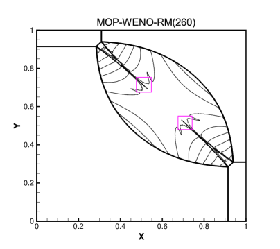
We calculate this problem using all the considered mapped WENO-X schemes in Table 1 and their corresponding MOP-WENO-X schemes. For the sake of brevity though, we only present the solutions of the WENO-M, WENO-IM(2, 0.1), WENO-PPM5, WENO-MAIM1 schemes and their corresponding MOP-WENO-X schemes in Figs. 13 and 14, where the first rows give the final structures of the shock and vortex in density profile of the existing mapped WENO-X schemes, the second rows give those of the corresponding MOP-WENO-X schemes, and the third rows give the cross-sectional slices of density plot along the plane $y=0.65$ where $x\in[0.70,0.76]$ . We find that all the considered schemes perform well in capturing the main structure of the shock and vortex after the interaction. It can be seen that there are clear post-shock oscillations in the solutions of the WENO-M, WENO-IM(2, 0.1) and WENO-PPM5 schemes. However, in the solutions of the MOP-WENO-M, MOP-WENO-IM(2, 0.1) and MOP-WENO-PPM5 schemes, the post-shock oscillations are either removed or significantly reduced. The post-shock oscillations of the WENO-MAIM1 scheme are very slight and even hard to be noticed. Actually, it seems difficult to distinguish the solutions of the WENO-MAIM1 scheme from that of the MOP-WENO-MAIM1 scheme only according to the structure of the shock and vortex in the density profile. Nevertheless, when taking a closer look from the cross-sectional slices of the density profile along the plane $y=0.65$ at the bottom right picture of Fig. 14 where the reference solution is obtained using the WENO-JS scheme with a uniform mesh size of $1600\times 1600$ , we can see that the post-shock oscillation of the WENO-MAIM1 scheme is very remarkable while it is imperceptible for the MOP-WENO-MAIM1 scheme. Also, from the third rows of Figs. 13 and 14, we find that the WENO-IM(2, 0.1) and WENO-PPM5 schemes generate the post-shock oscillations with much bigger amplitudes than that of the WENO-MAIM1 scheme. The WENO-M scheme also generates clear post-shock oscillations with the amplitudes slightly smaller than that of the WENO-IM(2, 0.1) and WENO-PPM5 schemes. Evidently, the solutions of the MOP-WENO-M, MOP-WENO-IM(2, 0.1) and MOP-WENO-PPM5 schemes almost generate no post-shock oscillations or only generate some imperceptible numerical oscillations and their solutions are very close to the reference solution, and this should be an advantage of the mapped WENO schemes whose mapping functions are OP.

Example 6

(2D Riemann problem) It is very favorable to test the high-resolution numerical methods [14, 15, 21] using the series of 2D Riemann problems [24, 23]. In [14], Lax et al. classified a total of 19 genuinely different Configurations for 2D Riemann problem and calculated all the numerical solutions. Configuration 4 is chosen here for the test, and the computational domain is initialized by

\big{(}\rho,u,v,p\big{)}(x,y,0)=\left\{\begin{aligned} \begin{array}[]{ll}(1.1,0.0,0.0,1.1),&0.5\leq x\leq 1.0,0.5\leq y\leq 1.0,\\ (0.5065,0.8939,0.0,0.35),&0.0\leq x\leq 0.5,0.5\leq y\leq 1.0,\\ (1.1,0.8939,0.8939,1.1),&0.0\leq x\leq 0.5,0.0\leq y\leq 0.5,\\ (0.5065,0.0,0.8939,0.35),&0.5\leq x\leq 1.0,0.0\leq y\leq 0.5.\\ \end{array}\end{aligned}\right.

The transmission boundary condition is used on all boundaries, and the numerical solutions are calculated on a uniform mesh size of $800\times 800$ . The computations proceed to $t=0.25$ .

Similarly, although we calculate this problem using all the considered mapped WENO-X schemes in Table 1 and their corresponding MOP-WENO-X schemes, we only present the solutions of the WENO-M, WENO-PM6, WENO-RM260 and MIP-WENO-ACM $k$ schemes and their corresponding MOP-WENO-X schemes here for the sake of brevity. We have shown the numerical results of density obtained by using these schemes in Figs. 15 and 16, where the first rows give the structures of the 2D Riemann problem in density profile of the existing mapped WENO-X schemes, the second rows give those of the corresponding MOP-WENO-X schemes, and the third rows give the cross-sectional slices of density plot along the plane $y=0.5$ where $x\in[0.65,0.692]$ . We can see that all schemes can capture the main structure of the solution. However, we can also observe that there are obvious post-shock oscillations (as marked by the pink boxes), which are unfavorable for the fidelity of the results, in the solutions of the WENO-M, WENO-PM6, WENO-RM(260) and MIP-WENO-ACM $k$ schemes. These post-shock oscillations can be seen more clearly from the cross-sectional slices of density profile as presented in the third rows of Figs. 15 and 16, where the reference solution is obtained by using the WENO-JS scheme with a uniform mesh size of $3000\times 3000$ . Noticeably, there are either almost no or imperceptible post-shock oscillations in the solutions of the MOP-WENO-M, MOP-WENO-PM6, MOP-WENO-RM(RM260) and MOP-WENO-ACM $k$ schemes. Again, we believe that this should be an advantage of the mapped WENO schemes whose mapping functions are OP.

5 Conclusions

The concept of OP-Mapped WENO schemes standing for the family of the mapped WENO schemes with order-preserving (OP) mappings, as well as a general way to build one group of this kind of schemes, has been proposed in this paper. Specifically, we extend the OP mapping introduced in [18] to various existing mapped WENO schemes in references by providing a general formula of their mapping functions. A systematic analysis has been made to prove that the improved mapped WENO scheme based on the existing mapped WENO-X scheme, denoted as MOP-WENO-X, generates numerical solutions with the same convergence rates of accuracy in smooth regions as the corresponding WENO-X scheme. Furthermore, numerical experiments are run to show that the MOP-WENO-X schemes have the same advantage as the mapped WENO scheme proposed in [18] in calculating the one-dimensional linear advection problems including discontinuities with long output times. The mapping functions of the MOP-WENO-X schemes are OP and hence able to attain high resolutions and avoid spurious oscillations meanwhile. Moreover, numerical results with the 2D Euler system problems were presented to show that the MOP-WENO-X schemes perform well in simulating the two-dimensional steady problems with strong shock waves to capture the main flow structures and remove or significantly reduce the post-shock oscillations.

References

Borges et al. [2008] R. Borges, M. Carmona, B. Costa, W.S. Don, An improved weighted essentially non-oscillatory scheme for hyperbolic conservation laws, J. Comput. Phys. 227 (2008) 3101–3211.
Chatterjee [1999] A. Chatterjee, Shock wave deformation in shock-vortex interactions, Shock Waves 9 (1999) 95–105.
Feng et al. [2012] H. Feng, F. Hu, R. Wang, A new mapped weighted essentially non-oscillatory scheme, J. Sci. Comput. 51 (2012) 449–473.
Feng et al. [2014] H. Feng, C. Huang, R. Wang, An improved mapped weighted essentially non-oscillatory scheme, Appl. Math. Comput. 232 (2014) 453–468.
Gottlieb and Shu [1998] S. Gottlieb, C.W. Shu, Total variation diminishing Runge-Kutta schemes, Math. Comput. 67 (1998) 73–85.
Gottlieb et al. [2001] S. Gottlieb, C.W. Shu, E. Tadmor, Strong stability-preserving high-order time discretization methods, SIAM Rev. 43 (2001) 89–112.
Harten [1989] A. Harten, ENO schemes with subcell resolution, J. Comput. Phys. 83 (1989) 148–184.
Harten et al. [1987] A. Harten, B. Engquist, S. Osher, S.R. Chakravarthy, Uniformly high order accurate essentially non-oscillatory schemes III, J. Comput. Phys. 71 (1987) 231–303.
Harten and Osher [1987] A. Harten, S. Osher, Uniformly high order accurate essentially non-oscillatory schemes I, SIAM J. Numer. Anal. 24 (1987) 279–309.
Harten et al. [1986] A. Harten, S. Osher, B. Engquist, S.R. Chakravarthy, Some results on uniformly high order accurate essentially non-oscillatory schemes, Appl. Numer. Math. 2 (1986) 347–377.
Henrick et al. [2005] A.K. Henrick, T.D. Aslam, J.M. Powers, Mapped weighted essentially non-oscillatory schemes: Achieving optimal order near critical points, J. Comput. Phys. 207 (2005) 542–567.
Hu et al. [2011] G. Hu, R. Li, T. Tang, A robust WENO type finite volumn solver for steady Euler equations on unstructured grids, Commun. Comput. Phys. 9 (2011) 627–648.
Jiang and Shu [1996] G.S. Jiang, C.W. Shu, Efficient implementation of weighted ENO schemes, J. Comput. Phys. 126 (1996) 202–228.
Lax and Liu [1998] P.D. Lax, X.D. Liu, Solution of two-dimensional Riemann problems of gas dynamics by positive schemes, SIAM J. Sci. Comput. 19 (1998) 319–340.
Li et al. [2015] Q. Li, P. Liu, H. Zhang, Piecewise Polynomial Mapping Method and Corresponding WENO Scheme with Improved Resolution, Commun. Comput. Phys. 18 (2015) 1417–1444.
Li and Zhong [2020] R. Li, W. Zhong, A modified adaptive improved mapped WENO method, arXiv preprint (2020) arXiv:2011.03916.
Li and Zhong [2021a] R. Li, W. Zhong, An efficient mapped WENO scheme using approximate constant mapping, arXiv preprint (2021a) arXiv:2102.00231.
Li and Zhong [2021b] R. Li, W. Zhong, A new mapped WENO scheme using order-preserving mapping, arXiv preprint (2021b) arXiv:2104.04467.
Liu et al. [1994] X.D. Liu, S. Osher, T. Chan, Weighted essentially non-oscillatory schemes, J. Comput. Phys. 115 (1994) 200–212.
Pao and Salas [1981] S.P. Pao, M.D. Salas, A numerical study of two-dimensional shock-vortex interaction, in: AIAA 14th Fluid and Plasma Dynamics Conference, California, Palo Alto, 1981.
Pirozzoli [2011] S. Pirozzoli, Numerical methods for high-speed flows, Annu. Rev. Fluid Mech. 43 (2011) 163–194.
Ren et al. [2003] Y.X. Ren, M. Liu, H. Zhang, A characteristic-wise hybrid compact-WENO scheme for solving hyperbolic conservation laws, J. Comput. Phys. 192 (2003) 365–386.
Schulz-Rinne [1993] C.W. Schulz-Rinne, Classification of the Riemann problem for two-dimensional gas dynamics, SIAM J. Math. Anal. 24 (1993) 76–88.
Schulz-Rinne et al. [1993] C.W. Schulz-Rinne, J.P. Collins, H.M. Glaz, Numerical solution of the Riemann problem for two-dimensional gas dynamics, SIAM J. Sci. Comput. 14 (1993) 1394–1414.
Shu [1998] C.W. Shu, Essentially non-oscillatory and weighted essentially non-oscillatory schemes for hyperbolic conservation laws, in: Advanced Numerical Approximation of Nonlinear Hyperbolic Equations. Lecture Notes in Mathematics, volume 1697, Springer, Berlin, 1998, pp. 325–432.
Shu and Osher [1988] C.W. Shu, S. Osher, Efficient implementation of essentially non-oscillatory shock-capturing schemes, J. Comput. Phys. 77 (1988) 439–471.
Shu and Osher [1989] C.W. Shu, S. Osher, Efficient implementation of essentially non-oscillatory shock-capturing schemes II, J. Comput. Phys. 83 (1989) 32–78.
Wang and Feng [2008] R. Wang, H. Feng, Observations on the fifth-order WENO method with non-uniform meshes, Appl. Math. Comput. 196 (2008) 433–447.
Wang et al. [2016] R. Wang, H. Feng, C. Huang, A New Mapped Weighted Essentially Non-oscillatory Method Using Rational Function, J. Sci. Comput. 67 (2016) 540–580.
Zhang et al. [2011] R. Zhang, M. Zhang, C.W. Shu, On the order of accuracy and numerical performance of two classes of finite volume WENO schemes, Commun. Comput. Phys. 9 (2011) 807–827.
Zhang and Shu [2007] S. Zhang, C.W. Shu, A new smoothness indicator for the weno schemes and its effect on the convergence to steady state solutions, J. Sci. Comput. 31 (2007) 273–305.