Towards an Improved Metric for Evaluating Disentangled Representations

In subsequent sections, we refer to latent dimensions as ‘codes’, and to the data generative factors as ‘factors’. Generative factors are those attributes that describe the perceptual differences between any two samples from dataset $\mathbf{X}$.

Consider a dataset $\mathbf{X}={\mathbf{x}^{(i)}}_{i=1}^{N}$ comprising $N$ i.i.d. samples. We assume these samples $\mathbf{x}$ are generated by a random process $g\mathrel{\mathop{\mathchar 58\relax}}\mathbb{R}^{k}\rightarrow\mathcal{X}$, which takes the ground truth generative factors $\mathbf{z}\in\mathbb{R}^{k}$ as input and returns the generated data $\mathbf{x}\in\mathcal{X}$. We now consider a latent variable model capable of inferring the corresponding latent representation $\mathbf{c}\in\mathbb{R}^{d}$ of the data $\mathbf{x}$. This latent representation $\mathbf{c}$, analogous to $\mathbf{z}$, can be used to generate the corresponding data $\mathbf{x}$. The model simulates the random process of generating data $\mathbf{x}$ as follows: latent variables $\mathbf{c}$ are sampled from some prior distribution $p_{\theta}(\mathbf{c})$, and then the data $\mathbf{x}$ is sampled from a conditional distribution $p_{\theta}(\mathbf{x}|\mathbf{c})$. The model aims to approximate the desired data distribution $p_{\theta}(\mathbf{x})=\int p_{\theta}(\mathbf{x}|\mathbf{c})p_{\theta}(\mathbf{c})d\mathbf{c}$.

Given the latent representations $\mathbf{c}$ learned by the trained latent variable model and the known ground truth generating factors $\mathbf{z}$, we aim to obtain a method to quantitatively evaluate the disentanglement of the latent space $\mathbb{R}^{d}$ by giving a certain score $s\in\mathbb{R}$ according to the identified definitions of disentanglement.

We measure the influence each of the factors $z_{i}$ have on the latent codes $c_{i}$ using a relationship matrix we call Impact Intensity. We introduce two improvements in the computation of relationship matrix, namely, a) an improved estimator and b) no reliance on ad-hoc decision model.

As pointed out earlier, existing implementations of MI in metrics are unsuited to high-dimensional continuous variables and fraught with computational challenges [15]. Naturally, a non-parametric estimator with no dependence on discretisation is more suitable. A recently proposed method called MINE [16] operates by training a small neural network to maximise a lower bound on the mutual information between two variables. As it involves no density estimation using maximum likelihood it is flexible and has been shown to converge to the true mutual information between high-dimensional variables [16]. Linearly scalable in both dimensionality and sample size, it offers a significant advantage (cf. Sections IV-B and IV-E).

Thus, we propose computing the relationship matrix as follows: First, we calculate the following required variables: a) $I(\bm{c}_{i};\bm{z}_{j})$, signifying the mutual information computed between each factor $\bm{c}_{i}$ and each code $\bm{z}_{j}$; b) $I(\bm{c}_{1},\bm{c}_{2},\dots,\bm{c}_{d};\bm{z}_{j})$, signifying the mutual information between all codes $\bm{c}_{1},\bm{c}_{2},\dots,\bm{c}_{d}$ and each factor $\bm{z}_{j}$; and c) $H(\bm{z}_{j})$, representing the entropy of each factor. We establish the relationship as $R(\bm{c}_{i};\bm{z}_{j})=\frac{I(\bm{c}_{i};\bm{z}_{j})}{I(\bm{c}_{1},\bm{c}_{2},\dots,\bm{c}_{d};\bm{z}_{j})}$, denoting the impact intensity of factor $\bm{z}_{j}$ on the code $\bm{c}_{i}$ among all codes. This, we argue, offers a more accurate representation of the relationship, as latent codes are learned from generative factors.

The concept of exclusivity is crucial in both modularity and compactness. In modularity, we desire a code to capture a singular factor and exclude others. In compactness, it is expected that a factor is represented by a code without overlapping with others. This principle is fundamentally the inverse of impurity.

We propose an intuitive method to quantify the extent of exclusivity, which is defined as the difference between correctness (the maximum value) and incorrectness (the root mean square error of all other values). The objective is to maximise the difference between correctness and incorrectness.

Given a set of attributes $\{a_{1},a_{2},\ldots,a_{n}\}$, the exclusivity is mathematically represented as:

	$\displaystyle\text{Exclusivity}(a_{1},a_{2},\ldots,a_{n})$	$\displaystyle=a_{i^{*}}-\sqrt{\frac{1}{n-1}\sum_{\begin{subarray}{c}i=1\\ i\neq i^{*}\end{subarray}}^{n}a_{i}^{2}},$
		$\displaystyle\quad\text{where}\quad i^{*}=\text{argmax}_{i}\,a_{i}.$

The aim is for the maximum value to be as high as possible, with the remainder as minimal as possible.

By applying the aforementioned concepts of exclusivity to better depict the “extent”, and impact intensity to capture factor-code relationships, we formulate the following metrics to measure modularity, compactness, and explicitness.

Modularity. We formalize the metric for modularity, or disentanglement, of a latent code $\bm{c}_{i}$ as:

$$D(\bm{c}_{i})=\text{Exclusivity}\left(\bm{R}(\bm{c}_{i};\bm{z}_{1}),\bm{R}(\bm{c}_{i};\bm{z}_{2}),\ldots,\bm{R}(\bm{c}_{i};\bm{z}_{k})\right).$$

The aggregate modularity score is then calculated as $D=\frac{1}{k}\sum_{i=1}^{d}D(\bm{c}_{i})$, where $d$ denotes the code dimensionality, and $k$, representing the number of factors, signifies the maximum potential influence a single factor can exert. Notably, this framework may encounter complications due to correlated effects, wherein multiple codes capture a single factor. To address this challenge, we allocate to each code $\bm{c}_{i}$ and its predominantly associated factor $\bm{z}_{j^{*}}$ a score $S_{ij^{*}}=D(\bm{c}_{i})$, while assigning $S_{ij}=0$ for $j\neq j^{*}$. Accumulating these scores across all factors yields $S_{j}=\sum_{i}S_{ij}$ for each factor $j$. Ensuring that the score for each factor does not exceed $1$ (the maximum conceivable impact intensity for each factor is $1$), the final score is thus recalculated as $D=\frac{\sum_{j}\max(S_{j},1)}{k}$, facilitating an accurate assessment of modularity.

We then assign a score $S_{ij^{*}}=D(\bm{c}_{i})$ to each code $\bm{c}_{i}$ and its most effective factor $\bm{z}_{j^{*}}$, and mark the others as $S_{ij}=0$ for $j\neq j^{*}$. The overall disentanglement is finally calculated as:

$$D=\frac{\sum_{j}{\min(S_{j},1)}}{k},\textrm{ where }S_{j}=\sum_{i}S_{ij}.$$

Compactness. The compactness of a generative factor $\bm{z}_{j}$ is calculated as:

$$C(\bm{z}_{j})=\text{Exclusivity}\left(\bm{R}(\bm{c}_{1};\bm{z}_{j}),\bm{R}(\bm{c}_{2};\bm{z}_{j}),\ldots,\bm{R}(\bm{c}_{d};\bm{z}_{j})\right).$$

Accordingly, the overall compactness score, $C$, is determined by the average compactness across all factors:

$$C=\frac{1}{k}\sum_{j=1}^{k}C(\bm{z}_{j}).$$

Explicitness. For a generative factor $\bm{z}_{j}$, explicitness or informativeness is calculated as the ratio of the combined information content of the codes relative to $\bm{z}_{j}$ to the entropy of $\bm{z}_{j}$ itself:

$$I(\bm{z}_{j})=\frac{I(\bm{c}_{1},\bm{c}_{2},\ldots,\bm{c}_{d};\bm{z}_{j})}{H(\bm{z}_{j})}.$$

Hence, the aggregate measure of informativeness is the mean informativeness across all generative factors:

$$I=\frac{1}{k}\sum_{j=1}^{k}I(\bm{z}_{j}).$$

Motivated by discrepancies in our exploratory analysis, we first systematically assess metric behaviour via discrete boundary test cases for each of the aspects i.e. modularity, compactness, and explicitness. Codes are arranged in that order with $1$ denoting a perfect aspect and $0$ completely imperfect. For example, $\#101$ indicates perfect disentanglement and explicitness, but imperfect compactness.

To form the factor space, we sample $N=50,000$ points from a discrete uniform distribution with a one-to-one encoding. Each category is assigned a distinct code $(k=d=2)$ unless: a) when modularity is low, we encode two factors into one code; b) when compactness is low, we encode a factor into two codes; or c) when informativeness is low, we randomly drop categories within the factors. We simulate a total of $2^{3}=8$ representative cases³³3detailed description in supplementary material. Results, reported in Table II using $s=50$ random seeds, confirm some intuitions, and previously reported observations while revealing interesting insights.

As discussed in Section II-4, not all metrics designed for specific aspects are well-calibrated. Z-min Variance, for instance, which is modularity-centric, fails to penalise modularity violations, with scores larger than 0.5 in low modularity scenarios ($\#000,\#001,\#010,\#011$). This stems from its assigning of the minimum score as $\frac{1}{d}$. The Modularity metric, while performing perfectly in high modularity cases, unexpectedly assigns high scores of 0.75 in low modularity scenarios too ($\#010$ and $\#011$). This is likely due to an error introduced by dividing the maximum term in the formula. DCI Mod correctly assigns low scores in low modularity cases of $\#000$ and $\#001$, however, it assigns relatively large scores of $>50\%$ in $\#010$ and $\#011$, indicating some influence of high compactness, which is not ideal. In contrast, EDI Mod assigns 0.43, reflecting low modularity relatively better.

The discrepancies appear in compactness-centric metrics as well. SAP, for instance, assigns a relatively low score of 0.33 in both high compactness scenarios ($\#010$ and $\#110$) but a higher score of 0.45 in the low compactness case of $\#101$, suggesting greater influence from other aspects. MIG also assigns relatively low scores of 0.41 and 0.45 in high compactness scenarios ($\#010$ and $\#110$), but a higher score of 0.49 in the less compact scenario of $\#101$. Its successor, MIG-sup, assigns a large score of 0.99 in both low ($\#100$, $\#101$) and high compactness scenarios ($\#110$, $\#111$) while tends to assign intermediate scores of about 0.5 in high compactness, low modularity scenarios ($\#010$). This shows a high influence from modularity but yields no clear interpretation of the captured aspects. Furthermore, the DCIMIG metric assigns a higher score to the low compactness case of $\#101$ confirming weak penalisation, as a consequence of two codes capturing different information extent about the factor. DCI Comp assigns very high scores to scenarios $\#100$ and $\#101$, which are highly modular despite low compactness. EDI Comp, in contrast, assigns lower scores. In terms of explicitness, EDI and DCI perform comparably. Overall the results indicate EDI to be better calibrated in comparison to the existing metrics.

The ability to attribute accurate scores when factor-code relationships are non-linear as in realistic data is a crucial property. A robust metric should exhibit negligible effect with increasing non-linearity. In this experiment, we simulate representations which are perfectly compact and modular, but the encoding function becomes increasingly non-linear. We use $f(z)$ = $1000-\alpha+0.25\tan\left(\omega(z-0.5)\right)+0.5$ where $\omega=2\arctan\left(1000\alpha-\frac{0.25}{2}\right)$. As $\alpha$ increases, the curve becomes more steep but remains monotonic for $z\in[0,1]$. Using $k=d=6$, we simulate $M=50$ representations with $N=20,000$ points sampled from $\mathcal{U}\in[0,1]$. For $s=50$ seeds, we report the aggregated scores in Figure 1.

This experiment perfectly challenges the complexity of the predictors employed by the metrics, and highlights the potential issues inherent to mutual information computation using density estimation, yielding interesting insights. Metrics that calculate MI using binning methods generally perform inadequately. To illustrate this, we contrasted MIG to its alternative variant implemented with a non-parametric estimator, KSG [15]. MIG-ksg demonstrates greater stability until reaching $\alpha=0.6$, after which it gradually declines. Metrics using linear models like SAP, exhibit instability as non-linearity increases. This is also observed in DCI, which in its original implementation uses a LASSO classifier. Both DCI Mod and Comp decline and become more variable as non-linearity increases. In contrast, Z-diff and Modularity scores exhibit stability throughout the experiment. EDI Mod and Comp consistently assign a perfect score of $1$ throughout too, indicating robustness in this setting. For explicitness, a slight reduction in mutual information is expected.

Next, we evaluate the performance of the metrics as a perfectly disentangled representation gradually transitions to an entangled state. We conduct an experiment where we linearly reduce the modularity and compactness of the representation while maintaining explicitness. To describe the factor-code relationship, we employ $f(\bm{z})=\bm{zR}$, with

$$\small\bm{R}=\begin{pmatrix}1-\alpha&\alpha&0&\cdots&0\\ 0&1-\alpha&\alpha&\cdots&0\\ \vdots&\ddots&\ddots&\ddots&\vdots\\ 0&\cdots&0&1-\alpha&\alpha\\ \alpha&0&\cdots&0&1-\alpha\end{pmatrix}.$$

Like in the previous experiment, we use $k=d=6$, and simulate $M=50$ representations with $N=20,000$ points. For $s=50$ seeds, we report the aggregated scores in  Figure 2. As the parameter $\alpha$ increases, we expect a linear decrease in all metrics dealing with modularity or compactness, though not reaching $0$ entirely⁴⁴4since increasing $\alpha$ does not lead to perfect entanglement, i.e. a factor equally represented by all codes. Instead, only two codes capture a factor.. Z-diff and Z-min Variance metrics fail completely in this regard. Conversely, both modularity and compactness components of EDI and DCI respectively demonstrate robust performance. DCI Expl, which does not represent true mutual information remains largely unaffected. It is also prone to overfitting and hence may overestimate explicitness [7]. In comparison, EDI Expl exhibits a drop when one factor becomes equally represented by two codes. Most information-based metrics also perform well, however, assign zero value already when only one factor or code becomes fully entangled.

In this segment, we investigate how the metrics behave when we keep modularity and compactness intact, but gradually reduce explicitness. Choosing $f(z)=(1-\alpha)z+\alpha n$, and keeping the setting consistent as before, we report the results in Figure 3. In this simulation, we expect the metrics representing explicitness to decrease gradually. In this regard, both EDI Expl and DCI Expl perform adequately, however unlike DCI, EDI Expl does not assign a perfect score of 1 here due to the true mutual information being less than 1. Metrics representing modularity and compactness should exhibit unchanged behaviour under noise. Here we see a larger contrast between the metrics. While MIG, SAP, and Modularity metric decrease gradually and reach 0, Z-min Variance collapses rapidly after the middle mark. DCI Mod and Comp also decrease, first slowly, then quite rapidly as $\alpha$ approaches $0.8$. Here we can see strikingly more stability in EDI Mod and Comp. In fact, even Z-diff appears to be robust here.

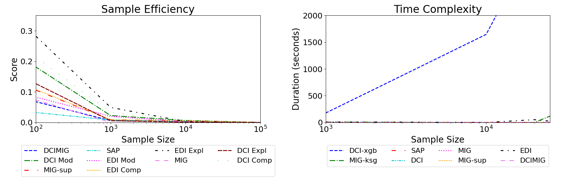
Here, we evaluate and compare the metrics in terms of sample efficiency and time complexity. To test sample efficiency, we compute the difference in estimated scores when using subsets of data $N\in\{100,1000,10000,10000\}$ against the full sample size of $N=100,000$. We keep the experimental setup as in section IV-A, with a difference that we use only 10 random seeds, and report the mean differences in Figure 4 (left). We observe the minimum samples required to reliably estimate scores vary across metrics, as a result of design choices. While most metrics converge around the 10,000 sample mark, it becomes evident that classifiers-based metrics such as DCI necessitate larger sample sizes for optimal performance, whereas metrics reliant on MI require fewer samples. In this regard, EDI generally is more sample-efficient than DCI, with the exception of its explicitness component, which needs more samples to reliably compute mutual information.

In terms of time complexity, most metrics are constant or (sub)linear. We observed EDI to be linear, and for DCI, it depends on the complexity of the ad-hoc model. If one were to choose complex models like random forest or XGBoost (DCI-xgb) to model non-linearity better as recommended [7], this would come with a serious disadvantage of the curse of dimensionality (cf. Figure 4 (right)).

It was observed in previous works that metrics do not correlate on complex datasets, and the correlations may not be consistent across datasets [13]. While we do not test consistency in this regard, we test general agreement of the metrics on a popular dataset used in the domain, namely Shapes3D⁵⁵5https://github.com/google-deepmind/3d-shapes, in order to test if EDI can be applied in real settings. We heuristically opted to utilise FactorVAE [11] and BetaVAE [10] for learning representations. For FactorVAE, we chose $\gamma\in\{2,4,6,8,10\}$, and for BetaVAE, $\beta\in\{2,3,4,5\}$. For $5$ random seeds, this resulted in $45$ representations in total. Next, we produce a ranking of the learned representations on the scores and calculate the agreement between the rankings for each pair of metrics using Spearman’s coefficient (cf. Figure 5).

We observe EDI to display strong correlations with SAP, DCIMIG, MIG-sup, Z-min Variance and perfect correlation with Modularity, indicating general agreement on both modularity and compactness aspects. The exception in this case is DCI which does not appear to correlate with most metrics. It might be that DCI required more hyperparameter tuning. MIG demonstrates a negative correlation with all metrics except EDI compactness. indicating that both measure similar properties to an extent.

References

- [1] Yoshua Bengio, Aaron Courville and Pascal Vincent “Representation Learning: A Review and New Perspectives” arXiv:1206.5538 [cs] arXiv, 2014 DOI: 10.48550/arXiv.1206.5538
- [2] Hagai Attias “Independent factor analysis” In Neural computation 11.4 MIT Press, USA, 1999, pp. 803–851
- [3] Cian Eastwood and Christopher K. I. Williams “A Framework for the Quantitative Evaluation of Disentangled Representations”, 2022 URL: https://openreview.net/forum?id=By-7dz-AZ
- [4] Karl Ridgeway and Michael C. Mozer “Learning Deep Disentangled Embeddings with the F-Statistic Loss” arXiv:1802.05312 [cs, stat] arXiv, 2018 URL: http://arxiv.org/abs/1802.05312
- [5] Abhishek Kumar, Prasanna Sattigeri and Avinash Balakrishnan “Variational Inference of Disentangled Latent Concepts from Unlabeled Observations” arXiv:1711.00848 [cs, stat] arXiv, 2018 DOI: 10.48550/arXiv.1711.00848
- [6] Ricky T. Q. Chen, Xuechen Li, Roger Grosse and David Duvenaud “Isolating Sources of Disentanglement in Variational Autoencoders” arXiv:1802.04942 [cs, stat] arXiv, 2019 URL: http://arxiv.org/abs/1802.04942
- [7] Marc-André Carbonneau, Julian Zaidi, Jonathan Boilard and Ghyslain Gagnon “Measuring Disentanglement: A Review of Metrics” arXiv:2012.09276 [cs] arXiv, 2022 URL: http://arxiv.org/abs/2012.09276
- [8] Anna Sepliarskaia, Julia Kiseleva and Maarten Rijke “How to Not Measure Disentanglement” arXiv:1910.05587 [cs, stat] arXiv, 2021 URL: http://arxiv.org/abs/1910.05587
- [9] Irina Higgins et al. “Towards a Definition of Disentangled Representations” arXiv:1812.02230 [cs, stat] arXiv, 2018 URL: http://arxiv.org/abs/1812.02230
- [10] Irina Higgins et al. “beta-VAE: Learning Basic Visual Concepts with a Constrained Variational Framework”, 2017 URL: https://openreview.net/forum?id=Sy2fzU9gl
- [11] Hyunjik Kim and Andriy Mnih “Disentangling by Factorising” arXiv:1802.05983 [cs, stat] arXiv, 2019 URL: http://arxiv.org/abs/1802.05983
- [12] Amir H. Abdi, Purang Abolmaesumi and Sidney Fels “A Preliminary Study of Disentanglement With Insights on the Inadequacy of Metrics”, 2019 arXiv:1911.11791 [cs.LG]
- [13] Francesco Locatello et al. “Challenging Common Assumptions in the Unsupervised Learning of Disentangled Representations” arXiv:1811.12359 [cs, stat] arXiv, 2019 URL: http://arxiv.org/abs/1811.12359
- [14] Zhiyuan Li, Jaideep Vitthal Murkute, Prashnna Kumar Gyawali and Linwei Wang “Progressive Learning and Disentanglement of Hierarchical Representations” arXiv:2002.10549 [cs, stat] arXiv, 2020 URL: http://arxiv.org/abs/2002.10549
- [15] Alexander Kraskov, Harald Stögbauer and Peter Grassberger “Estimating mutual information” In Phys. Rev. E 69 American Physical Society, 2004, pp. 066138 DOI: 10.1103/PhysRevE.69.066138
- [16] Mohamed Ishmael Belghazi et al. “MINE: Mutual Information Neural Estimation”, 2021 arXiv:1801.04062 [cs.LG]
-A Existing Metric Formulations
-A1 Z-diff (BetaVAE) Metric
Higgins et al. [10] introduced the BetaVAE based on the notion that dimensions capturing the constant generative factor should match, while others vary. This metric aims to capture modularity by computing the following steps:
-
(a)
Selecting a generative factor .
(b)
Choosing a pair of samples, and , with constant while other factors vary.
(c)
Generating latent codes and .
(d)
Calculating pairwise distortion:
(1) -
(e)
Repeating the above steps to train a linear classifier predicting the fixed generative factor, with Z-diff indicating classifier precision.
-A2 Z-min Variance (FactorVAE) Metric
Kim et al. [11] proposed a metric similar to Z-diff, based on the assumption that latent codes capturing a constant generative factor should remain consistent. The method normalises each latent code by its dataset-wide standard deviation. The latent dimension with the least variance and the index of the constant factor form a sample for a linear classifier, assessing the classifier’s precision.
-A3 Separated Attribute Predictability (SAP)
Kumar et al. [5] developed the SAP metric, based on a matrix of informativeness , with each entry representing a linear regression from latent code to generative factor . The SAP score is: