Towards accurate nuclear mass tables in covariant density functional theory
Abstract
The current investigation focuses on detailed analysis of the anchor based optimization approach (ABOA), its comparison with alternative global fitting protocols and on the global analysis of the truncation of basis effects in the calculation of binding energies. It is shown that ABOA provides a solution which is close to that obtained in alternative approaches but at small portion of their computational time. The application of softer correction function after few initial iterations of ABOA stabilizes and speeds up its convergence. For the first time, the numerical errors in the calculation of binding energies related to the truncation of bosonic and fermionic bases have been globally investigated with respect of asymptotic values corresponding to the infinite basis in the framework of covariant density functional theory (CDFT). These errors typically grow up with the increase of the mass and deformation of the nuclei. To reduce such errors in bosonic sector below 10 keV for almost all nuclei with proton number one should truncate the bosonic basis at instead of presently used . The reduction of the errors in binding energies due to the truncation of the fermionic basis in CDFT is significantly more numerically costly. For the first time it is shown that the pattern and the speed of the convergence of binding energies as a function of the size of fermionic basis given by depend on the type of covariant energy density functional. The use of explicit density dependence of the meson-nucleon coupling constants or point couplings slows down substantially the speed of convergence of binding energies as a function of . The present paper clearly indicates the need for accounting of infinite basis corrections for accurate calculation of binding energies and for fitting more precise next generation covariant energy density functionals: note that such corrections are neglected in the present generation of the functionals. A new procedure for finding the asymptotic values of binding energies is suggested in the present paper: it allows better control of numerical errors.
I Introduction
Nuclear binding energies (or masses) is one of the most fundamental properties of atomic nuclei. In experiment they are studied with extreme relative mass precision of and in some nuclei even with precision of Mittig et al. (2003); Dilling et al. (2018). In absolute terms this corresponds to the accuracy of the measurements of the binding energies better than 1 keV. Accurate knowledge of binding energies is important for nuclear structure, neutrino physics and nuclear astrophysics. The measurements of nuclear masses far from stability provide a fundamental test for our understanding of nuclear structure Mittig et al. (2003) and the constraints on model predictions for the boundaries of nuclear landscape (see Ref. Erler et al. (2012); Afanasjev et al. (2013); Agbemava et al. (2014)). The measurements of mass differences ( values) of specific isotopes play a key role in neutrino physics: in order to determine the neutrino mass on a sub-eV level one should measure the values of certain transitions better than 1 eV Dilling et al. (2018). Different nuclear astrophysical processes [such as r-process (see Refs. Arnould et al. (2007); Cowan et al. (2021)) or the processes in the crust of neutron stars (see Refs. Chamel and Haensel (2008); Lau et al. (2018))] also sensitively depend on nuclear masses since they affect nuclear reaction rates.
There was a substantial and continuous effort in non-relativistic models to improve the functionals and global reproduction of experimental masses (see, for example, Refs. Tondeur et al. (2000); Samyn et al. (2002); Goriely et al. (2013); Baldo et al. (2013); Möller et al. (2016); Kortelainen et al. (2010, 2012, 2014) and references quoted therein). Existing global fits of the model parameters to the ground state masses reach an accuracy of MeV in the global reproduction of experimental masses in the microscopic+macroscopic (mic+mac) approach Möller et al. (2016) and in Skyrme density functional theory (DFT) Goriely et al. (2013) and around 0.8 MeV in the Gogny DFT Goriely et al. (2009). These fits take into account the correlations beyond mean field by either adding rotational and vibrational corrections in a phenomenological way or by employing five-dimensional collective Hamiltonian (5DCH). Note that the global fits at the mean field level in the Skyrme DFT lead to MeV accuracy in the global description of experimental binding energies (see Refs. Kortelainen et al. (2010, 2012, 2014)).
In contrast, the attempts to create covariant energy density functionals (CEDF) based on the global set of data on binding energies are very limited in covariant density functional theory (CDFT). It is only in Refs. Peña-Arteaga et al. (2016); Taninah and Afanasjev (2023) that they were undertaken (see Sec. II for more detail). This is due to the fact that the calculations within the CDFT are significantly more numerically challenging and more time-consuming as compared with those carried out in nonrelativistic DFT due to relativistic nature of the CDFT. First, the wavefunctions of the single-particle states in the CDFT are represented by Dirac spinors the large and small components of which have opposite parities. As a consequence, the basis for a given maximum value of principal quantum number in the basis set expansion has approximately double size in the CDFT as compared with non-relativistic models. As a result, the numerical calculations of matrix elements and the diagonalization of the matrices requires substantially more time than in the case of nonrelativistic DFTs. A rough estimate provided in Ref. Reinhard et al. (1986) for spherical symmetry indicates that the calculations in the Skyrme DFT and CDFT for a given maximum value of principal quantum number in the basis set expansion differ by approximately an order of magnitude. Second, the most widely used classes of CEDFs contain the mesons in addition to fermions Vretenar et al. (2005); Agbemava et al. (2014). This requires the solution of Klein-Gordon equations which adds numerical cost to the calculations. Third, in the CDFT the nucleonic potential ( MeV/nucleon) emerges as the sum of very large attractive scalar ( MeV/nucleon) and repulsive vector ( MeV/nucleon) potentials (see Ref. Vretenar et al. (2005)). In the nucleus with mass , these values are multiplied by and this leads to a cancellation of very large quantities. This may lead to a slower convergence of binding energies as a function of the size of the basis in the CDFT as compared with non-relativistic DFTs.
Many of the fits of the relativistic and non-relativistic functionals (including global ones) have been carried out using computer codes employing basis set expansion approach in which the wave functions are expanded into the basis of harmonic oscillator wave functions. This expansion is precise for the infinite size of the basis. However, due to numerical reasons the basis is truncated in the calculations. Unfortunately, a rigorous analysis of numerical errors in calculated binding energies emerging from the truncation of basis is missing in global calculations. However, there are some indications that they are not negligible. For example, the relativistic Hartree-Bogoliubov (RHB) calculations of the ground state in 208Pb with DD-ME2 functional indicate that binding energies calculated with fermionic shells deviate from asymptotic value of binding energy by approximately 250 keV (see discussion of Fig. 2 in Supplemental Material to Ref. Taninah and Afanasjev (2023)). Note that this difference represents only 0.015% error in the description of total binding energy. In a similar way, total binding energies of the 120Sn and 102,110Zr nuclei obtained in the Skyrme DFT calculations with the SLy4 force in the basis of and harmonic oscillator (HO) shells differ by 110-150 keV Dobaczewski et al. (2004); Pei et al. (2008). Ref. Pei et al. (2008) also indicates that the HO basis with is needed in order to describe the binding energies of the nuclei in this mass region with an accuracy of the couple of tens keV.
Thus, the present paper aims at the investigation of several issues related to the calculations of binding energies with high precision in the CDFT framework. One of the goals is to understand the numerical errors in the calculations of binding energies. In particular, their global dependence on the truncation of the basis both in the fermionic and bosonic sectors of the CDFT will be investigated for the first time. We will also study how these numerical errors depend on the type of the symmetry (spherical versus axially deformed) of the nuclear shape and how the convergence of binding energies as a function of the size of the basis depends on the type of functional. The second goal is to understand to which extent the procedures for the definition of asymptotic binding energies employed earlier in non-relativistic functionals are applicable in the CDFT. The third goal is to further understand the role and the features of the anchor based optimization method suggested in Ref. Taninah and Afanasjev (2023) as an alternative to other methods of global fitting of the functionals.
The paper is organized as follows. A short review of the approaches to global fitting of the energy density functionals (EDF) is presented in Sec. II. Sec. III provides a brief outline of theoretical formalism and the discussion of major classes of CEDFs under study. A discussion of the anchor based approach to the optimization of energy density functionals and its comparison with alternative methods for global fitting of the functionals is given in Sec. IV. The impact of the truncation of basis in bosonic and fermionic sectors of the CDFT on binding energies as well as asymptotic behavior of the calculated binding energies are analysed in Sec. V. A new method of defining asymptotic values of calculated binding energies is presented in Sec. VI. Finally, Sec. VII summarizes the results of our paper.
II A review of approaches to global fitting of functionals
The analysis of literature reveals that at present there are three different approaches to global fitting of energy density functionals. These are
-
•
Fully Global Approach (further FGA). In the FGA the optimization of the functional is performed using computer codes which include either axial or triaxial deformation. It allows to use in fitting protocol the quantities which depend on deformation such as fission barriers which are not accessible in alternative fitting protocols.
-
•
Reduced Global Approach (further RGA) has been outlined in Sec. II of Ref. Tondeur et al. (2000). The specific feature of this approach is the fact that the deformation effects are taken into account in deformed and transitional nuclei by calculating the deformation energy
(1) where is the energy at the equilibrium deformation and is the energy of spherical configuration. The values are calculated using axially deformed code and then all experimental binding energies are renormalized to their ”equivalent spherical configuration” values. Then, the rms errors of the current iteration of the functional are calculated using a spherical code by comparing the binding energies it gives with these renormalized experimental binding energies. Thus, each iteration of optimization consists of defining the in deformed code and fitting the functional in spherical code. However, to reach an optimal fit one should repeat iterations until full convergence of is reached.
-
•
Anchor Based Optimization Approach (further ABOA). In the ABOA (see Ref. Taninah and Afanasjev (2023)), the optimization of the parameters of EDFs is carried out for a selected set of spherical anchor nuclei, the physical observables of which are modified by the correction function
(2) which takes into account the global performance of EDFs. Here is the counter of the iteration in the anchor-based optimization. The parameters and correct the deficiencies of EDF in isospin and in mass number while is responsible for a global shift in binding energies111Note that similar in spirit approach is used in Ref. Gonzalez-Boquera et al. (2018) in which the quadrupole zero-point energy is replaced by a constant binding energy shift [similar to the term in Eq. (2)] which is fixed by minimizing the global rms deviation..
Each of these approaches has its own advantages and disadvantages which are discussed below.
The FGA potentially allows to avoid all uncertainties related to the selection of nuclei used in the fitting protocol and allows to use the physical quantities which depend on deformation (such as the height of fission barriers) in fitting protocol. However, the calculations in deformed codes are extremely numerically expensive and computational time does not depend drastically on the selection of the functional (see Table 1). For example, within the CDFT framework the numerical calculations in deformed RHB code are by more than two orders of magnitude more time consuming than those in spherical RHB one for the fermionic basis characterized by full fermionic shell (see columns 4 and 5 in Table 2). Further increase of fermionic basis leads to a drastic increase of the ratio of the calculational time in deformed and spherical RHB calculations: this ratio is approaching three orders of magnitude at (see Table 2).The simplification of the code by the transition to the relativistic mean field (RMF)+BCS framework does not change much this ratio. Similar situation holds also in non-relativistic Skyrme and Gogny DFT.
| Computational time per nucleus [CPU-hours] | ||||
| DD-MEX | DD-PC1 | NL5(E) | PCPK1 | |
| 16 | 0.26 | 0.15 | 0.19 | 0.19 |
| 18 | 0.51 | 0.35 | 0.40 | 0.39 |
| 20 | 1.05 | 0.68 | 0.68 | 0.68 |
| 22 | 2.02 | 0.98 | 1.43 | 1.22 |
| 24 | 3.36 | 2.02 | 2.57 | 2.66 |
| 26 | 5.17 | 4.08 | 4.48 | 4.20 |
| 28 | 8.21 | 6.39 | 7.77 | 7.49 |
| 30 | 15.94 | 11.11 | 13.34 | 11.66 |
| Computational time | Ratio | |||
|---|---|---|---|---|
| per nucleus [CPU-hours] | ||||
| 2 | 3 | 4 | 5 | |
| DD-MEX | DD-PC1 | DD-MEX | DD-PC1 | |
| 16 | 0.000440 | 0.000238 | 590.91 | 630.25 |
| 18 | 0.000596 | 0.000365 | 855.70 | 958.90 |
| 20 | 0.000646 | 0.000590 | 1625.39 | 1152.54 |
| 22 | 0.001233 | 0.000700 | 1638.28 | 1400.00 |
| 24 | 0.001654 | 0.000953 | 2031.44 | 2119.62 |
| 26 | 0.002163 | 0.001264 | 2390.20 | 3227.85 |
| 28 | 0.002401 | 0.001634 | 3419.41 | 3910.65 |
| 30 | 0.002758 | 0.001983 | 5779.55 | 5602.62 |
The FGA has been used in the number of studies but there are two possible ways of its application. In the first method, a large basis is used to reduce numerical errors in the calculations of binding energies but this restricts the number of the nuclei which can be included in the fitting protocol. However, the lack of strict mathematical procedure in the selection of nuclei leads to some subjectivity and possibly to some biased errors. This problem can be reduced by the inclusion of a larger set of nuclei into the fitting protocol. However, the computational cost raises drastically so that the increase of the number of nuclei leads to a substantial reduction of the basis size used in the calculations because of the limitations imposed on availability of computational resources. This, in turn requires the use of approximate relations to find the asymptotic value of the binding energy corresponding to infinite size of basis (see Sec. V for details). Thus, a very large number of the nuclei is used in the fitting protocol of the second method but this requires the use of moderate basis in numerical calculations and approximate relations to find the asymptotic value of the binding energy corresponding to infinite size of basis.
For example, the first method was used in Refs. Kortelainen et al. (2010, 2012, 2014) in Skyrme DFT for the development of the UNEDF class of the functionals. Note that fitting protocol of the UNEDF1 and UNEDF2 functionals has been supplemented by information on fission barriers and single-particle energies, respectively. In all optimizations, the large spherical basis with 20 harmonic oscillator shells () was used which led to quite substantial computational time in the calculations with deformed HFBTHO code. As a consequence, a limited number of nuclei (approximately 28 spherical and 46 deformed) were used in these optimizations.
The second method has been used in the fitting protocol of the BCPM (Barcelona-Catania-Paris-Madrid) functional (see Ref. Baldo et al. (2013)). It included 579 measured masses of even-even nuclei and the calculations have been carried out in a reduced basis which takes into account eleven harmonic oscillator shells for the nuclei, 13 shells for the nuclei, and 15 shells for nuclei. Another example is the D1M and D1M* functionals which were fitted to 2149 and 620 nuclei, respectively, in axially deformed calculations corrected by quadrupole corrections to total binding energy and infinite-basis corrections [see Eq. (27) below] in Refs. Goriely et al. (2009); Gonzalez-Boquera et al. (2018). Note that only even-even nuclei were considered in the fit of the D1M* functional. The axially deformed calculations for these two functionals were performed in the basis with major oscillator shells.
There is also a hybrid method which was used in the fitting of the DD-MEB1 and DD-MEB2 CEDFs in Refs. Peña-Arteaga et al. (2016): this fitting protocol contains 2353 experimental masses. The minimization of these functionals was performed in axially deformed RHB code with fermionic shells but with calculated binding energies corrected before and after minimization by the difference between the results obtained with and (see Ref. Goriely (2023a)).
The RGA has been used in the fitting protocol of the BSk1-32 series of the Skyrme functionals using very large bases (see, for example, Refs. Samyn et al. (2002); Goriely et al. (2013, 2016); Goriely (2023b)). For instance, it consisted of the HO shells in spherical calculations and HO shells in deformed calculations in Ref. Samyn et al. (2002). This allows to keep numerical error in calculated masses relatively low without involving the correction for infinite basis size. Note that fitting protocols of these functionals typically include all nuclei for which experimental data on binding energies is available.
The ABOA has been introduced in Ref. Taninah and Afanasjev (2023). It was shown that the use of this approach leads to a substantial improvement in the global description of binding energies for several classes of CEDFs (see also Sec. IV.1 below). This approach leads to the results which are comparable to those obtained in RGA (see Ref. Taninah and Afanasjev (2023) and the discussion in Sec. IV.3). The computational cost of defining a new functional within this approach is drastically lower as compared with FGA and RGA and this aspect is discussed in detail in Sec. IV.2 below. It turns out that the use of twelve anchor spherical nuclei distributed over the nuclear chart in the optimization is sufficient for this approach (see Ref. Taninah and Afanasjev (2023)). Note that existing optimizations of CEDFs within the ABOA have been obtained in the RHB calculations with fermionic and bosonic shells (see Ref. Taninah and Afanasjev (2023)). Such a truncation of the basis is used also in other recent CEDF optimizations222Unfortunately, the majority of the papers dedicated to the optimization of CEDFs do not explicitly provide information on the size of the basis used in the fitting protocols. (see, for example, Refs. Zhao et al. (2010); Taninah et al. (2020)). However, there are also the cases when smaller basis was used: for example, the DD-PC1 functional has been defined in deformed calculations with fermionic shells Nikšić et al. (2008).
It is necessary to mention that in these investigations the numerical errors in the binding energies associated with the truncation of basis or the definition of their asymptotic values have been either discussed only for a few selected nuclei or not mentioned at all. Thus, at present there is no published information on how these errors evolve across the nuclear landscape and how they depend on the type of the functional or theory employed. Thus, one of the goals of the present study is to close this gap in our knowledge in the CDFT framework.
III Theoretical framework
The calculations were performed in the framework of relativistic Hartree-Bogoliubov (RHB) approach the technical details on the solution of which can be found in Refs. Vretenar et al. (2005); Agbemava et al. (2014); Nikšić et al. (2014). The calculations were carried out with two versions of the RHB code suitable for spherical and axially deformed nuclei, respectively. Both codes allow the calculations with a wide range of covariant energy density functionals. We employ a parallel version of the axial RHB computer code developed in Ref. Agbemava et al. (2014): it allows simultaneous calculations for a significant number of nuclei and deformation points in each nucleus. The unconstrained calculations are performed in axial RHB code using four initial deformations of the basis and 0.4. As follows from the comparison with the calculations constrained on this procedure guarantees finding the lowest in energy minimum but it is substantially less numerically costly as compared with constrained calculations.
Both spherical and axial RHB computer codes are based on the expansion of the Dirac spinors and the meson fields in terms of harmonic oscillator wave functions with respective symmetry [so-called basis set expansion method] (see Ref. Gambhir et al. (1990); Nikšić et al. (2014)). We illustrate here this expansion for the case of axially deformed nuclei (see Refs. Gambhir et al. (1990); Nikšić et al. (2014) for more details and for the case of spherical symmetry).
The single-particle wave function of the nucleon in the state , which follows from the solution of the Dirac equation, is given by
| (3) |
where the large () and small () components of a Dirac spinor are expanded independently in terms of the HO eigenfunctions
| (4) | |||
| (5) |
The HO eigenfunctions have the form (see Ref. Nikšić et al. (2014))
| (6) |
where and are the number of nodes in the - and - directions, respectively, and and are projections of the orbital angular momentum and spin on the intrinsic -axis, respectively. and are oscillator lengths in respective directions.
The quantum numbers and in the sums of Eqs. (4) and (5) run over all permitted combinations of and , and (and their tilted counterparts) defined by the truncation of the basis. In absolute majority of the CDFT calculations, full fermionic HO shells are used in the basis set expansion and we follow this prescription in the present paper. Thus, is selected in such a way that all basis states corresponding to full fermionic shells are included into the basis of large components. The basis of small components includes full fermionic shells to avoid spurios contributions to the RHB equation (see Ref. Gambhir et al. (1990) for details). Note that large and small components of the Dirac spinor have opposite parities: this leads to an approximate doubling of the basis in the CDFT as compared with non-relativistic theories.
The solution of the Klein-Gordon equation is obtained by expanding mesonic fields in a complete set of basis states [HO eigenfunctions] along [] and perpendicular [ the axis of symmetry of the nucleus
| (7) |
This expansion is truncated at full bosonic shells.
The spherical RHB code is not parallelized but it allows the calculations to a very large value of (see Sec. V.2 below). Thus, the convergence of the results of the calculations in spherical nuclei as a function of has been tested using this code. In contrast, the axial RHB code works only up to due to memory allocation problems at larger values of . Note that similar to Fig. 2 of Supplemental Material to Ref. Taninah and Afanasjev (2023) we verified for selected set of spherical and deformed nuclei that the codes developed in our group and those existing in the DIRHB package of the RHB codes (see Ref. Nikšić et al. (2014)) provide almost the same (within a few keVs) results for binding energies as a function of and . Note that only DD-ME* and DD-PC* types of the functionals are included into the DIRHB codes of Ref. Nikšić et al. (2014).
In order to understand the dependence of the convergence properties on the functional we consider three major classes of CEDFs used at present. These are (i) those based on meson exchange with non-linear meson couplings (NLME) (see Ref. Boguta and Bodmer (1977)), (ii) those based on meson exchange with density dependent meson-nucleon couplings (DDME) (see Ref. Typel and Wolter (1999)), and finally (iii) those based on point coupling (PC) models containing various zero-range interactions in the Lagrangian (see Ref. Bürvenich et al. (2002)).
The Lagrangians of these three major classes of CEDFs can be written as: where the consist of the Lagrangian of the free nucleons and the electromagnetic interaction. It is identical for all three classes of functionals and is written as
| (8) |
with
| (9) |
and
| (10) |
For each model there is a specific term in the Lagrangian: for the DDME models we have
| (11) | |||||
with the density dependence of the coupling constants given by
| (12) | |||||
| (13) |
where denotes the saturation density of symmetric nuclear matter and . The functions are given by the Typel-Wolter ansatz Typel and Wolter (1999)
| (14) |
Because of the five conditions , , and , only three of the eight parameters , , , and are independent and we finally have the four parameters , , , and characterizing the density dependence. In addition we have the four parameters of the Lagrangian , , , and . As usual the masses of the - and the -meson are kept fixed at the values MeV and MeV Lalazissis et al. (2005); Roca-Maza et al. (2011). We therefore have parameters in the DDME class of the models. The DD-MEX Taninah et al. (2020), DD-ME2 Lalazissis et al. (2005) and DD-MEY Taninah and Afanasjev (2023) functionals have been used in the present study.
The NLME class of the functionals has the same model specific Lagrangian as the DDME class except that the coupling constants , , and are constants and there are extra terms for a non-linear meson coupling. These couplings are important for the description of surface properties of finite nuclei, especially the incompressibility Boguta and Bodmer (1977) and for nuclear deformations Gambhir et al. (1990).
| (15) |
For the NLME class we have parameters , , , , , and . In the present study, we use the NL5(E) CEDF from Ref. Agbemava et al. (2019a).
In general, the Lagrangian of the PC models contains three parts:
(i) the four-fermion point coupling terms:
| (16) |
(ii) the gradient terms which are important to simulate the effects of finite range:
| (17) |
(iii) The higher order terms which are responsible for the effects of medium dependence
| (18) |
However, the structure of two PC functionals, namely, PC-PK1 and DD-PC1, employed in the present paper depends on particular realization of this scheme. The PC-PK1 CEDF closely follows this scheme but it neglects the scalar-isovector channel, i.e. . This is because the information on masses and charge radii of finite nuclei does not allow one to distinguish the effects of the two isovector mesons and (see Ref. Roca-Maza et al. (2011)). Thus, for this PC CEDF we have parameters , , , , , , , , . The DD-PC1 functional Nikšić et al. (2008) introduces the density dependence of the , and constants via
and eliminates the terms proportional to , [this is similar to the PC-PK1 functional] and , , , and in Eqs. (16-18). The introduced density dependence of the , and constants partially takes care of the impact of omitted terms. Note that in the isovector channel a pure exponential dependence is used, i.e. . Thus, the DD-PC1 functionals contains the parameters, i.e. , , , , , , , , and .
Note that in the deformed RHB calculations we use and integration points in the Gauss-Hermite and Gauss-Laguerre quadratures in the and directions, respectively, in order to properly take into account the details of the single-particle wave functions. The same is used in the Gauss-Hermite quadratures for in spherical RHB calculations.
The experimental binding energies of twelve anchor spherical nuclei (16O, 40,48Ca, 72Ni, 90Zr, 116,124,132Sn, 204,208,214Pb and 210Po) and charge radii of nine of them (namely, 16O, 40,48Ca, 90Zr, 116,124Sn and 204,208,214Pb) are used in the anchor based optimization approach (see Ref. Taninah and Afanasjev (2023) for more details). The correction function of Eq. (2) is defined in ABOA using 855 even-even nuclei for which experimental binding energies are available in Ref. Wang et al. (2017).
IV Further discussion of anchor-based optimization approach
The anchor-based optimization of energy density functionals is defined in Ref. Taninah and Afanasjev (2023) and the basic results for this approach have been discussed in this reference and in Supplemental Material to it. It is based on the introduction of the correction function given in Eq. (2) by which the binding energies of spherical anchor nuclei are redefined for global performance of the EDFs (see Ref. Taninah and Afanasjev (2023)) for full details). The behavior of these parameters during the iterative procedure has been illustrated for the DD-MEX1, DD-MEY and NL5(Y) functionals in Tables I, II and III of the Supplemental Material to Ref. Taninah and Afanasjev (2023). In addition, the evolution of the rms deviations between calculated and experimental binding energies for these functionals during the iterative procedure was also illustrated in Fig. 1 of Supplemental Material to Ref. Taninah and Afanasjev (2023).
In this section we extend the discussion of the ABOA to other functionals, introduce new improved strategy for the fitting of the functionals within ABOA, provide an estimate of the computation time for the ABOA and RGA approaches and compare the results obtained for the DD-MEY type of the functionals in the RGA and ABOA.
IV.1 Further improvement of the convergence of the ABOA
Figure 1 of Supplemental Material to Ref. Taninah and Afanasjev (2023) [see also black curve in Fig. 1(c)] shows a significant increase in global at the 4th iteration of the convergence process. This indicates that the push provided by the correction function of Eq. (2) is too strong. It turns out that this problem can be eliminated by switching to a softer correction function
| (20) |
after few initial iterations in the convergence process. Note that the convergence of the iterative procedure is reached in the limit , , and .
The advantage of this modified procedure is illustrated in Fig. 1(c) on the example of the DD-MEX1 functional. The use of correction function leads to the convergence curve for shown in black color which is characterized by a large peak at the iteration and which requires 14 iterations for a convergence. However, the switch to at the 3d iteration eliminates this peak and reduces the number of required iterations to seven (see red curve in Fig. 1(c) and Table 3). Thus, the combination of these two correction functions leads to a rapid and smooth convergence process: the function provides a significant push so that only one to three iterations are needed to drive the functional towards its minimum in the parameter hyperspace in the beginning of iterative process and guaranties the smoothness of convergence process at further iterations.
This combined procedure has also been used in the fit of the PC-Y and PC-Y1 functionals defined in Ref. Taninah and Afanasjev (2023). Figs. 1(a) and (b) and Tables 4 and 5 illustrate that drastic improvement of the global performance of these functionals was reached after first iteration and then additional few iterations provide only minor improvement of the functionals.
| iteration | ||||
|---|---|---|---|---|
| [MeV] | ||||
| 0 | 2.849 | -0.075 | 0.0235 | -3.29 |
| 1 | 2.144 | 0.044 | -0.028 | 2.55 |
| 2 | 2.139 | -0.044 | 0.026 | -2.12 |
| 3 | 1.799 | 0.045 | -0.020 | 1.70 |
| 4 | 1.653 | 0.005 | 0.000 | 0.05 |
| 5 | 1.654 | 0.005 | 0.000 | 0.05 |
| 6 | 1.675 | -0.010 | 0.000 | 0.00 |
| 7 | 1.651 | 0.000 | 0.000 | 0.00 |
| iteration | ||||
|---|---|---|---|---|
| [MeV] | ||||
| 0 | 3.097 | +0.086 | -0.036 | 1.00 |
| 1 | 1.974 | -0.003 | +0.002 | -0.25 |
| 2 | 1.951 | -0.002 | +0.001 | -0.15 |
| 3 | 1.959 | 0.000 | 0.000 | -0.19 |
| 4 | 2.002 | -0.007 | 0.001 | -0.13 |
| 5 | 1.950 | 0.009 | 0.004 | -0.14 |
| 6 | 1.951 | -0.0099 | 0.004 | 0.02 |
| iteration | ||||
|---|---|---|---|---|
| [MeV] | ||||
| 0 | 2.698 | +0.065 | -0.030 | 1.10 |
| 1 | 1.943 | -0.010 | 0.000 | 0.20 |
| 2 | 1.953 | -0.010 | -0.001 | 0.15 |
| 3 | 1.923 | +0.024 | -0.001 | -0.03 |
| 4 | 1.858 | +0.017 | -0.002 | 0.01 |
| 5 | 1.849 | +0.001 | -0.0001 | -0.001 |


IV.2 The dependence of computational time on approach
It is interesting to compare the computer resources required for definition of the functional in different approaches. The numbers quoted below are based on the RHB calculations with and . Numerical calculations are performed at Orion of High Performance Computing Collaboratory (HPC2) of Mississippi State University (see https://www.hpc.msstate.edu/computing/hpc.php) and they reflect the computation time allocation of this facility. The largest standard allocation per user is 400 CPU with 48 hours execution time limit; it is utilized in most of our calculations.
Let us start with anchor based optimization approach. The first step in each iteration of ABOA is the optimization of the parameters for 12 anchor spherical nuclei. This is carried out within the simplex method333The simplex method of the minimization is one of the simplest and fastest ones (see Ref. Press et al. (2007)). The minimizations by the simplex method are prone to end in local minima and that is a reason why, in general, it is not recommended for the search of the global minimum. However, it is our experience that by starting from a reasonable number of randomly generated initial points in parameter hyperspace we always find a global minimum as defined by alternative approaches such as simulated annealing method (see also Refs. Taninah et al. (2020); Taninah and Afanasjev (2023)). Note that this number depends on the size of parameter hyperspace. In contrast, the simulated annealing method is extremely costly and numerically unstable for large parameter hyperspaces: in our experience it works reasonably well only in a narrow parameter hyperspace around the global minimum and even then it is by an order of magnitude more time consuming than the simplex method. Note that the simplex method also provides the access to parametric correlations in the functionals (see Ref. Taninah et al. (2020)). starting from 200 randomly generated initial points in the large parameter hyperspace at the 0th iteration of ABOA. At subsequent iterations of ABOA the number of randomly generated initial points is decreased to 20 since the parameter hyperspace, which is centered around minimum found at previous iteration and in which the solution is sought, is made smaller.
On average, each minimization of the parameters for 12 spherical anchor nuclei requires approximately 3200 iterations in the optimization process and 8 hours of CPU time are allocated for it444The optimization is performed in parallel computer code. Thus, the computation time for each optimization iteration is defined by the nucleus the calculation of which takes the longest time. This is because the penalty function is defined at the end of each iteration the calculation of which requires the information on each nucleus included in the fitting protocol.. Thus, the total allocated computation time for this step is 12 nuclei times 20 runs times 8 CPU hours per run which results into 1920 CPU hours for iterations 1, 2, … of ABOA. Note that computation time allocation is ten times larger for the iteration of ABOA.
The calculations of each of 855 deformed nuclei requires the allocation of 4 CPU hours per run and they are carried out for 4 deformations of basis. This results in the allocation of CPU hours.
Thus, the 0th iteration and each subsequent iteration of ABOA require the allocation of 19200+13680=32880 and 1920+13680=15600 CPU hours, respectively. The experience with several types of the functionals tells us that approximately six iterations of ABOA are required to define the functional (see Sec. IV.1 and Supplemental Material to Ref. Taninah and Afanasjev (2023)). Thus, in total approximately 126400 CPU hours are required for the definition of the functional in the anchor-based optimization. This is only approximately six times more time-consuming than in the typical fitting protocol restricted to 12 spherical nuclei used in Ref. Taninah et al. (2020) and which corresponds to the optimization of anchor spherical nuclei in the 0th iteration of ABOA.
The next approach is the RGA one. Because of the process of job allocation at HPC2, it is possible to calculate maximum 400 nuclei in parallel. The optimization of 400 ”spherical” nuclei in the RGA approach is significantly more time consuming than twelve ones in ABOA because of three reasons discussed below. First, the number of ”spherical” nuclei is approximately 33 times larger. Second, the CPU time per nucleus in optimization process is significantly larger in the RGA approach than in the ABOA one. This time is defined in parallel calculations by the nucleus the calculation of which takes the longest time since the penalty function is defined at the end of iteration when the information on all nuclei are collected. In that respect, the 12 spherical nuclei used in ABOA are extremely well behaved with fast convergence in numerical calculations in part because the pairing collapses either in one or in both subsystems. In contrast, the pairing is present in most of the nuclei used in the RGA approach and numerical calculations converge slowly in some of these nuclei. Third, because of larger set of nuclei in the RGA approach as compared with ABOA, the optimization of ”spherical” nuclei requires larger number of iterations in the minimization process (around 8000) and the allocation of 24 hours per run. Note that similar to ABOA, we use simplex method for minimization with 20 randomly generated initial points in the parameter hyperspace. As a result, one round of optimization of spherical nuclei in the RGA requires CPU hours.
The calculations of deformed nuclei in the RGA are less numerically costly but they have to be done twice: the deformed RHB calculations without constraint on deformation for each nucleus with four initial deformations of basis for the definition of the energy of global minimum and deformed RHB calculations with constraint on spherical shape and with only spherical deformation of basis for the definition of the energy of spherical solutions. Thus the calculational time for deformed nuclei is 400 nuclei times 4 CPU hours per run times 4 runs for different deformations of basis for finding global minima plus 400 nuclei times 4 CPU hours per run for finding spherical solutions; altogether that is 8000 CPU hours.
Thus, one iteration of optimization in the RGA for 400 nuclei requires the allocation of approximately 200000 CPU hours. This is somewhat larger than the time required for defining the functional in the ABOA. If to scale this number to 855 nuclei (as in the ABOA), this would lead to approximately 427500 CPU hours.

However, to achieve an optimal solution one should perform a number of iterations of RGA to ensure that the deformation energies converge. In order to find how many iterations of RGA are needed for that we carried out the calculations for the CEDFs the fitting protocols of which are the same as for the DD-MEX1 and DD-MEY functionals defined in Ref. Taninah and Afanasjev (2023). The convergences of the error in deformation energies for these functionals are shown in Fig. 2. It was very slow for the DD-MEX1 type of the functional. The best MeV value has been achieved at the iteration of the RGA (see Fig. 2). However, this value is large and that is a reason why the process has been interrupted after four iterations for this functional. The convergence of the errors is better in the DD-MEY type of the functional (see Fig. 2) but even for this functional no full convergence of is reached after eight iterations of RGA. Note that the absence of full convergence of deformation energies affects mostly the nuclei in which the deformation is well pronounced (see Fig. 3). Fig. 2 clearly illustrates that substantial number of additional iterations of RGA would be required for a full convergence of deformation energies. Note that iterative processes shown in this figure were interrupted because of extreme numerical cost: one iteration of RGA is as expensive as a full fit of the functional in ABOA.
It was shown in Refs. Agbemava et al. (2019a); Taninah et al. (2020) that there are correlations between the parameters of state-of-the-art CEDFs: one can speak of parametric correlations between the parameters and when the parameter , with a reasonable degree of accuracy, can be expressed as a function of the parameter . The simplest type of such correlations which exists in CEDFs is a linear one given by
| (21) |
where
| (22) |
Here is the value of the parameter in the functional variation and is the value of the parameter in the optimal functional (see Ref. Taninah et al. (2020) for detail).
The removing of such correlations allows to reduce the number of free parameters in CEDFs (see Refs. Agbemava et al. (2019a); Taninah et al. (2020)). Here by using the DD-MEY type of the functionals as an example we will evaluate the impact of the removing of parametric correlations on computational time and convergence of deformation energies in RGA. Using the procedure of Ref. Taninah et al. (2020) one can establish the following correlations between the , and parameters
| (23) | |||
| (24) |
Thus, the removing of parametric correlations leads to a reduction of the number of free parameters in the DD-MEY type of functionals from 8 to 6. The functional with built-in correlations of Eqs. (23) and (24) is called as DD-MEY(par).
As a consequence of this reduction of the number of adjustable parameters, the time required for one round of optimization of spherical nuclei is reduced by approximately 30%. However, the results labelled as ”DD-MEY(par)” in Fig. 2 show that the removing of parametric correlations does not improve substantially the convergence of deformation energies.

Taking all these facts into account one can conclude that RGA is by more than one order of magnitude numerically more time consuming than ABOA and its performance strongly depend on how many iterations of RGA are required for the convergence of deformation energies. However, the latter is strongly dependent on the functional.
FGA approach requires the use of deformed code for the calculations of all nuclei included in the fitting protocol. At present, we did not make any calculations in the FGA but a crude estimate can be obtained by comparing the calculational time for the same set of nuclei carried out in spherical and deformed RHB codes. As discussed earlier, the most of numerical cost in the ABOA and RGA calculations are related to the calculations of spherical nuclei. In contrast, the numerical cost in FGA is defined by the cost of the calculations of deformed nuclei. Let us assume that (i) the same set of the nuclei is used in the RGA and FGA and (ii) the number of iterations in the optimization is comparable for the calculations with spherical and deformed RHB codes. Then, the results presented in the columns 4 and 5 of Table 2 will clearly indicate that the numerical cost of FGA will be larger than that in a single iteration of RGA555Here we compare full FGA with a single iteration of RGA since FGA does not require the calculation of deformation energies. by more than three orders of magnitude at fermionic basis with and this cost difference will rapidly increase with increasing .
Note that utilized calculational time is substantially lower than allocated time since many processes finish before the end of allocated time. Utilization rate defined as a ratio of actual calculational time versus allocated one can be improved by a further optimization of the structure of computer codes to the structure of run/time allocation at the HPC2. However, in no way it will significantly change the ratio of the computational times of the ABOA, RGA and FGA.
There is an additional issue related to the stability of numerical calculations for the nuclei included into fitting protocol which have not been discussed in the literature on CDFT. The importance of this factor can be illustrated by comparing the parameters of the PC-PK1 and PC-X functionals in Table 3 of Supplemental Material in Ref. Taninah et al. (2020). These two functionals have the same fitting protocols. However, both and parameters have opposite signs in these functionals and the penalty function obtained in PC-X is almost by a factor of two better than the one obtained in PC-PK1. A careful analysis reveals that numerical solutions for the pair of very light nuclei included into fitting protocol are unstable at some steps of minimization which in the end leads to non-convergence of the minimization process in a specific volume of parameter hyperspace. Note that this problem has been taken care in the minimization of the PC-X functional by using simplex method starting from large set of randomly generated initial points in the parameter hyperspace. This example clearly indicates that it is beneficial to use in fitting protocols the nuclei in which the numerical solutions behave well. This not only ensures the stability of the minimization process but also enlarges the parameter hyperspace in which the optimum solution can be sought and reduces computational time of minimization. In this respect, a very small set of twelve nuclei included in the fitting protocol of ABOA are extremely well behaved in numerical calculations.
IV.3 DD-MEY functional: ABOA versus RGA
It is important to understand to which extent the ABOA could be a reasonable substitute to a significantly more numerically time-consuming RGA. To do that we carried out RGA calculations using the same experimental information (restricted to binding energies and charge radii) and the isospin-dependent pairing as in the fitting protocol of the DD-MEY CEDF in ABOA (see Ref. Taninah and Afanasjev (2023) for details). The computational procedure discussed in Sec. IV.2 was used in these calculations.
| DD-MEY | DD-MEY(3) | DD-MEY(6) | |
|---|---|---|---|
| ABOA | RGA | RGA | |
| 1 | 2 | 3 | 4 |
| [MeV] | 1.734 | 1.672(0.068) | 1.725(0.074) |
| [fm] | 0.0264 | 0.0294 | 0.0303 |
| [MeV] | -16.09 | -16.044 | -16.017 |
| [fm-3] | 0.1529 | 0.1522 | 0.1545 |
| [MeV] | 265.8 | 261.6 | 248.5 |
| [MeV] | 32.8 | 31.6 | 30.1 |
| [MeV] | 51.8 | 42.6 | 29.5 |
| [MeV] | 551.321796 | 552.291521 | 551.989284 |
| 10.411867 | 10.398001 | 10.315743 | |
| 12.803298 | 12.758552 | 12.648663 | |
| 3.692170 | 3.548208 | 3.325439 | |
| 2.059712 | 2.249514 | 2.148238 | |
| 3.210289 | 3.551463 | 3.464883 | |
| 3.025356 | 3.437551 | 3.284163 | |
| 0.532267 | 0.652200 | 0.859341 |
When comparing the results of the RGA and ABOA calculations one should keep in mind that due to limited computational power the results of the RGA are always a subject of an error in deformation energies. However, these errors are acceptable (below 150 keV for in considered cases) so that the comparison of these two approaches is feasible. Table 6 presents such a comparison between ABOA and RGA results for two iterations of RGA [with respective functionals labelled as DD-MEY(2) and DD-MEY(5)] characterized by values of 0.068 and 0.074 MeV, respectively.
One can see that the parameters , and presented in Table 6 are very similar for the series of the DD-MEY* functionals obtained in different calculational schemes. Such a localization of these parameters in parameter hyperspace is typical for all functionals which include meson exchange and it is a consequence of the fact that nucleonic potential is defined as a sum of very large attractive scalar and repulsive vector potentials (see Refs. Agbemava et al. (2019a); Taninah et al. (2020)). In contrast, other parameters such as , , , and in Table 6 show somewhat larger relative spreads as compared with , and since for acceptable functionals they are less localized in the parameter hyperspace (see Refs. Agbemava et al. (2019a); Taninah et al. (2020)).
However, considering different sets of the nuclei included in the fitting protocols of RGA (400 nuclei) and ABOA (12 nuclei) and the remaining errors in the deformation energies in the RGA calculations, one can conclude that both ABOA and RGA lead to comparable functionals which provide similar global accuracy of description of binding energies ( MeV) and charge radii ( fm) (see Table 6). Note also that the predicted nuclear matter properties (NMP) of these functionals are within the ranges fm-3, MeV, , MeV ( MeV) and () for the SET2a (SET2b) sets of the constraints on the experimental/empirical ranges for the quantities of interest recommended for relativistic functionals in Ref. Dutra et al. (2014). This is the first time that a good reproduction of strict SET2b constraints has been achieved in CDFT by fitting only binding energies and charge radii of finite nuclei: the fitting protocol of DD-MEY* does not contain any information on NMP (see Supplemental Material to Ref. Taninah and Afanasjev (2023)).
IV.4 Charge radii in ABOA
A general expression for a charge radius in the CDFT is given by Horowitz and Piekarewicz (2012); Kurasawa and Suzuki (2019)666The analysis of the contributions of the last two terms of this expression in non-relativistic DFTs is presented in Refs. Friar and Negele (1975); Reinhard and Nazarewicz (2021); Naito et al. (2021). There are some differences between relativistic and non-relativistic treatments of these terms (see detailed discussion in Ref. Kurasawa and Suzuki (2019)), however, in general a comparable modification of charge radii is generated by such terms in relativistic and non-relativistic DFTs.
| (25) |
where stands for point-proton mean square radius as emerging from the CDFT calculations, and are mean-square charge radii of single proton and neutron, respectively, and and are proton and neutron spin-orbit contributions to the charge radius.
The situation with neutron mean-square charge radius is currently settled: the weighed average of few experiments provides fm2 Zyla et al. (2020) and the value fm2 is used in recent studies of charge radii within Skyrme DFT and CDFT frameworks (see Refs. Horowitz and Piekarewicz (2012); Kurasawa and Suzuki (2019); Reinhard and Nazarewicz (2021)). In contrast, there are some uncertainties in the definition of the proton mean-square charge radius which are generally discussed in the literature as proton radius puzzle (see Refs. Sick (2018); Gao and Vanderhaeghen (2022)). This puzzle is known as a discrepancy between proton radius obtained from muonic hydrogen spectroscopy which provides fm (see Ref. Zyla et al. (2020); Gao and Vanderhaeghen (2022)) and that derived from elastic electron-proton scattering which give a larger value of fm Sick (2018). It is still not fully resolved and future experiments are required to remove this discrepancy in (see Ref. Gao and Vanderhaeghen (2022)).
| DDMEY | NL5(Y) | |||
| Calculational | Anchor | Global | Anchor | Global |
| scheme | ||||
| fm | ||||
| Scheme-A | 0.0143 | 0.0218 | 0.0179 | 0.0294 |
| Scheme-B | 0.0162 | 0.0253 | 0.0190 | 0.0308 |
| Scheme-C | 0.0186 | 0.0253 | 0.0217 | 0.0308 |
| fm | ||||
| Scheme-A | 0.0201 | 0.0241 | 0.0228 | 0.0295 |
| Scheme-B | 0.0129 | 0.0223 | 0.0163 | 0.0297 |
| Scheme-C | 0.0144 | 0.0223 | 0.0203 | 0.0297 |
| fm | ||||
| Scheme-A | 0.0284 | 0.0291 | 0.0304 | 0.0334 |
| Scheme-B | 0.0151 | 0.0217 | 0.0181 | 0.0272 |
| Scheme-C | 0.0147 | 0.0217 | 0.0185 | 0.0272 |
To our knowledge all existing CEDFs were fitted with fm and only with first two terms in Eq. (25) (see discussion in Ref. Perera et al. (2021)): this corresponds to Scheme-A discussed below. Thus, it is important to evaluate the significance of these limitations as well as those connected with proton radius puzzle on the results for the nuclei included in the fitting protocol and on global results. This is done in Table 7 which compares the results obtained with three calculational schemes, namely,
-
•
Scheme-A: only first two terms of Eq. (25) are included,
-
•
Scheme-B: only first three terms of Eq. (25) are included,
-
•
Scheme-C: all terms of Eq. (25) are taken into account in the calculations of charge radii of twelve spherical anchor nuclei included in anchor-based optimization. Such results are shown in the columns labelled as ”ABOA” in Table 7. In contrast, only three first terms of Eq. (25) are taken into account in the global calculations which also include transitional and deformed nuclei. This is based on the assessment of Ref. Reinhard and Nazarewicz (2021) that such approximate relation is sufficient in the applications which aim at global description of charge radii777The spin-orbit contribution to charge radii decreases with increasing the mass of nuclei and it almost does not depend on the CEDF. These features are illustrated in Table II of Ref. Horowitz and Piekarewicz (2012). Since the calculations of this reference are restricted to spherical shape and neglect the pairing correlations, the values quoted for spin-orbit contribution to charge radii in this table for non-doubly magic nuclei have to be considered as an upper limit. This is because the deformation and pairing give rise to the mixing of different spherical subshells in the structure of the single-particle states which results in a smoothing of the spin-orbit correction to charge radii as a function of particle number Reinhard and Nazarewicz (2021). As a consequence, the charge radii in only restricted number of light nuclei are moderately affected by spin-orbit contributions (see Refs. Horowitz and Piekarewicz (2012); Kurasawa and Suzuki (2019)). Thus, Ref. Reinhard and Nazarewicz (2021) suggested to ignore last two terms of Eq. (25) in global analysis of charge radii.. As a result, the global results obtained in Scheme-B and Scheme-C calculations are identical.
and with three values of , 0.8409 and 0.887 fm. In addition, the calculations are performed with two CEDFs, namely, DD-MEY and NL5(Y) in order to see the dependence of the results on the functional.
The column ”Anchor” of Table 7 shows the results for the nuclei included in typical fitting protocol of anchor-based optimization approach (see Ref. Taninah and Afanasjev (2023)) which contains 12 nuclei and only 10 of them, namely, 16O, 40,48Ca, 90Zr, 116,124,132Sn and 204,208,214Pb provide the information on charge radii. In the column ”Global” we compare the results of the calculations for the set of 261 even-even nuclei in which experimental data on charge radii exist. Note that our set is reduced as compared with the 351 even-even nuclei listed in the compilation of Ref. Angeli and Marinova (2013) because of the reasons discussed below. For example, we exclude the nuclei with proton number since with the exception of uranium nuclei there are no direct experimental measurements of the absolute charge radii of such nuclei: the data for these nuclei provided in the compilation of Ref. Angeli and Marinova (2013) is based on extrapolations. Moreover, we exclude from consideration the nuclei in which beyond mean field and shape coexistence effects have substantial impact on charge radii. These are, for example, the nuclei, the Pb and Hg isotopes with , the Sr, Kr, and Mo isotopes with (see Ref. Perera et al. (2021)). Thus, we focus on the nuclei for which the absolute values of charge radii are experimentally measured888It is sufficient to measure the absolute value of charge radius of a single nucleus in isotopic chain and then to establish the charge radii of other nuclei in the chain by means of laser spectroscopy (see Ref. Campbell et al. (2016)). and for which mean field approximation is expected to be a reasonable well justified.
The analysis of the results presented in Table 7 leads to the following conclusions. First, the comparisons of the results obtained with fm and 0.887 fm in different calculational schemes clearly indicate that the uncertainties in the value of lead to the uncertainties in rms charge radii. The latter are the largest for calculational Scheme-A in which they are located between 0.0039 fm and 0.0083 fm dependent on the functional and on whether Anchor or Global results are compared. This provides a potential limit on the accuracy with which the charge radii can be meaningfully calculated at present. Further improvement of the description of charge radii below this limit requires the resolution of proton radius puzzle.
Second, Table 7 reveals clear correlations between rms deviations obtained in the Anchor and Global calculations: for a given functional and the calculational scheme with the lowest value in Anchor calculations provides either the lowest or comparable with the lowest value in Global calculations. This clearly indicates that the use of twelve anchor spherical nuclei in ABOA ten of which contain experimental information on charge radii is sufficient for constraining the properties of charge radii globally.
Note that the extension of the dataset of the nuclei with charge radii used in the fitting protocol beyond these ten nuclei will not necessary improve the agreement with experiment on a global scale because of increased theoretical uncertainties in the description of charge radii of the ground states. Indeed, charge radii sensitively depend on the underlying single-particle structure (see Refs. Perera et al. (2021); Naito et al. (2022); Perera and Afanasjev (2023)) the accuracy of the description of which typically reduces on going on from spherical to deformed nuclei (see, for example, Refs. Bonneau et al. (2007); Litvinova and Afanasjev (2011); Dobaczewski et al. (2015)). In addition, in the case of the nuclei with shape coexistence or soft potential energy surfaces the beyond mean effects have to be taken into account and their inclusion in model description is extremely numerically costly. Thus, the restriction of the dataset of the nuclei with charge radii used in the fitting protocol to spherical predominantly single and doubly magic ones reduces theoretical uncertainties related to the shape of the nucleus and underlying single-particle structure. However, for these nuclei the inclusion of the last three terms of Eq. (25) is important for further improvement of the functionals.
V Asymptotic behavior of the binding energies: basis truncation effects

The values of and employed in the RMF+BCS or RHB calculations depend on available computational power [which increases with time] and on the approach of theory group to handling the numerical errors in physical observables. In absolute majority of such calculations, is fixed at 20 since the calculations in bosonic sector of the models are relatively cheap. In contrast, the size of the fermionic basis shows substantial variations and dependence on time of publication, the sophistication of theoretical approach and theory group since the cost of numerical calculations in the RMF+BCS and RHB approaches is mostly defined by this sector.
Let us briefly review truncation schemes of fermionic basis of existing global mass calculations in the CDFT framework. Note that we specify below only if it differs from 20. The value has been used in global RMF+BCS mass calculations with NL3 CEDF in Ref. Lalazissis et al. (1999) with a larger number of fermionic shells used in very heavy nuclei. The RMF+BCS calculations of Ref. Geng et al. (2005) have been carried with and TMA CEDF. Global RMF+BCS calculations with CEDFs NL3, TM1, FSUGold and BSR4 were performed in Ref. Reinhard and Agrawal (2011) with . was used in global RHB calculations with the DD-ME2, DD-PC1, NL3* and DD-ME functionals in Ref. Agbemava et al. (2014). Ref. Zhang et al. (2014) presents the results of the global RMF+BCS calculations with phenomenological treatment of the dynamical correlation energy and CEDF PC-PK1: it uses for nuclei and for heavier ones. The transition to microscopic beyond mean field approaches leads to a significant increase of computational time. As a consequence, the fermionic basis is reduced in such studies. For example, the first global investigation within five-dimensional collective Hamiltonian (5DCH) based on triaxial RMF+BCS calculations with PC-PK1 CEDF employs , 14 and 16 for the nuclei with , , and , respectively (see Ref. Lu et al. (2015)). The same fermionic basis is used in the 5DCH studies based on triaxial RHB calculations with PC-PK1 CEDF presented in Ref. Yang et al. (2021).
While the majority of these schemes of the truncation of the fermionic basis provide a sufficient accuracy for absolute majority of physical observables (such as radii, deformations, etc) it is still an open question on how accurate they are for the calculations of the binding energies. This is because the assessment of the accuracy of the truncation of the basis in these publications has been either not carried or performed by comparing the solutions obtained with and (or as in Ref. Agbemava et al. (2014)) for very restricted set of nuclei. As a consequence, a number of the issues has not even been considered in earlier publications. For example, how the truncation errors in binding energies depend on the type of the functional? Or what is the evolution of truncation errors with proton and neutron numbers? Are those errors gradually increase with particle numbers or there are some local fluctuations caused by the shell effects?
To address these questions one should consider an asymptotic limit for the binding energies 999 is the (negative) binding energy of the nucleus with protons and neutrons. which corresponds to and . The asymptotic (negative) binding energy corresponding to these limits is defined as and it serves as a benchmark with respect of which the truncation errors in binding energies in the basis with () have to be defined. The consideration of this limit and related truncation errors are presented below for bosonic and fermionic sectors separately.
V.1 Bosonic sector
Since the bosonic basis size grows modestly with the absolute majority of the RMF+BCS and RHB calculations have been performed with starting from 90ites of the last century. For most of physical observables, this basis provides a required accuracy. However, we are not aware of any publication in which the convergence of binding energies as a function of has been presented. Fig. 4 and Table 8 fills this gap in our knowledge and shows the dependence of the difference between the calculated binding energies and on the number of bosonic shells for selected set of spherical nuclei ranging from light to superheavy ones. The binding energies obtained in the calculations with and do not differ by more than 1 keV both in spherical and deformed calculations. Thus, their average is treated as . Note that fermionic basis is fixed at in these calculations. To illustrate the dependence of the convergence of binding energies with increasing on the functional, the calculations are carried out with for CEDFs DD-ME2 Lalazissis et al. (2005) and DDMEX Taninah et al. (2020), which are similar in structure but somewhat different in numerical values of the parameters.
The convergence pattern of binding energies as a function of depends on the nucleus. For example, the 40Ca and 100Sn nuclei are more bound at low ( as compared with asymptotic limit which they gradually reach with increasing [see Fig. 4(a) and (e)]. In contrast, the 132Sn nucleus is less bound ( at than asymptotic limit, then it becomes slightly more bound for , and finally approaches asymptotic limit [see Fig. 4(f)]. Similar but inverted behavior is seen in 78Ni [see Fig. 4(d)]. If to exclude the results at , the 208Pb nucleus is less bound than in asymptotic limit for but calculated binding energies are close to asymptotic limit at higher [see Fig. 4(g) and (h)].
The convergence of the results to asymptotic limit only weakly depends on the functional [see Table 8]. Few keV accuracy is achieved globally with , in sub-lead () region with and in tin and sub-tin () region with . With increasing mass number, the accuracy of a given truncation of bosonic basis decreases. For example, the truncation scheme with is accurate up to 1 keV in 40Ca in both functionals. However, its accuracy drops to keV in superheavy 304120 nucleus. Note that the sign of fluctuates across the nuclear chart for a given : this means that in some nuclei a given truncation scheme provides more bound and in others less bound solutions as compared with asymptotic ones (see also Fig. 4).
The numerical errors in the description of binding energies increase on transition from spherical to deformed nuclei. This is illustrated in Table 9 on the example of selected deformed rare-earth, actinide and superheavy nuclei. For example, the use of , 24 and 28 in rare-earth 162Sm, 164Dy and 170Yb nuclei leads to keV, keV and a few keV errors in the description of binding energies, respectively. These errors somewhat increase on transition to actinides (240,250Pu) and superheavy (272Ds, 278Cn) nuclei so that it is required to use basis to achieve keV errors in these nuclei. Note that the errors in the light and medium mass () nuclei which are not shown in Table 9 are substantially lower than those in rare-earth region.
Considering the patterns of the behavior of with increasing shown in Fig. 4 (such as those in 132Sn), the extrapolation relations (similar to those discussed in Sec. V.2) based on small size of bosonic basis can suffer from numerical errors. Thus, taking into account the modest increase of basis size with , it is better to use large basises (such as ) for precise mass calculations. This will lead only to modest increase of computational time and memory requirements as compared with case and can be easily handled on modern high-performance computers.
| Nuclei | DD-ME2 | DD-MEX | ||||
|---|---|---|---|---|---|---|
| B(20) | B(24) | B(28) | B(20) | B(24) | B(28) | |
| 40Ca | 0.72 | -0.24 | 0.02 | 0.10 | -0.63 | -0.14 |
| 48Ca | 0.90 | -0.87 | -0.15 | -1.23 | -1.90 | -0.30 |
| 56Ni | 1.10 | -1.99 | -0.34 | -3.83 | -3.90 | -0.56 |
| 78Ni | 3.23 | 0.72 | 0.09 | -2.79 | -0.07 | -0.37 |
| 100Sn | 3.42 | -0.95 | -1.60 | -1.69 | -5.65 | -3.22 |
| 132Sn | -12.74 | 1.98 | 0.61 | -28.73 | -3.42 | 0.21 |
| 208Pb | -4.25 | -9.00 | 2.03 | 19.58 | -17.34 | -0.86 |
| 130.96 | 6.59 | -2.09 | 135.33 | 21.95 | -4.98 | |
| Nuclei | DD-ME2 | DD-MEX | ||||
|---|---|---|---|---|---|---|
| B(20) | B(24) | B(28) | B(20) | B(24) | B(28) | |
| 162Sm | -36.38 | 2.93 | 0.85 | -48.83 | -4.76 | 0.24 |
| 164Dy | -40.53 | 0.49 | 0.98 | -56.03 | -9.89 | -0.12 |
| 170Yb | -50.78 | -1.59 | 1.59 | -53.59 | -13.79 | 0.73 |
| 240Pu | -33.94 | -25.39 | 0.00 | -0.49 | -34.30 | -4.40 |
| 250Pu | 11.48 | -10.50 | -5.01 | 35.89 | -10.74 | -8.79 |
| 272Ds | -33.33 | -24.17 | -11.84 | -10.13 | -17.70 | -16.60 |
| 278Cn | -57.37 | -11.48 | -13.06 | -38.33 | -6.47 | -15.63 |
V.2 Fermionic sector
V.2.1 Binding energies

The asymptotic values of binding energy are extremely numerically expensive to calculate and we are not aware about any attempts in the CDFT framework apart of those presented in Refs. Agbemava et al. (2019b); Taninah and Afanasjev (2023) for a few nuclei to obtain or to approach these values by a drastic increase of the basis size beyond the one (typically ) used in global calculations of binding energies. To address this issue we carried out the calculations for selected sets of spherical and deformed nuclei, the representative cases of which are discussed below.
The evolution of both the calculated binding energy and the quantity [defined below] as a function of number of fermionic shells is considered here. The quantity
| (26) |
provides a more accurate measure of the convergence process since it compares the binding energies in the calculations with and . The convergence is reached when with increasing .
The results of the calculations for the evolution of these quantities with the increase of for a few selected spherical and deformed nuclei are presented in Figs. 5 and 6, respectively. A few general conclusions emerge from the analysis of the results of these calculations.
First, the binding energy can either decrease or increase on approaching its asymptotic value and this process depends on CEDFs. For , the absolute value of binding energy increases for the functionals which contain point coupling (PC-PK1 and DD-PC1) while it decreases for CEDFs which contain meson exchange (NL5(E), DD-ME2 and DD-MEX). This trend can be disturbed and reversed at lower in medium and heavy mass nuclei [see, for example, Fig. 5(e)] leading to the fluctuations of binding energies at .
Second, the convergence speed depends on the functional (see right panels of Figs. 5 and 6). In a given nucleus, the fastest convergence (at lower ) is reached by the NL5(E) functional. This follows by the DD-ME2 and DD-MEX functionals which typically require a few extra fermionic shells as compared with NL5(E) for a full convergence. The point coupling functionals are characterized by the slowest convergence since they require additional fermionic shells for a full convergence as compared with the DD-ME* ones. Note that in superheavy 304120 nucleus no full convergence is reached with PC functionals even with in spherical RHB calculations [see Figs. 5(e)].

Third, the convergence speed depends on the mass of the nucleus (see right panels of Figs. 5 and 6). For example, spherical solution converges at , and in the calculations with NLME, DDME and PC functionals in 40Ca [see Figs. 5(b)]. However, to reach a comparable level of convergence one should have , and in 132Sn [see Fig. 5(d)]. The required number of shells increases further for superheavy 304120 nucleus: the convergent solution is approached at in the calculations with NL5(E) functional and at in the calculations with the DDME functionals [see Fig. 5(f)]. Note that the PC functionals do not fully converge even at .
Fourth, some additional increase of the size of fermionic basis is required for a full convergence of the RHB solutions as a function of in deformed nuclei. This is illustrated in Fig. 6. Note that because of the memory allocation limits one can carry out axially deformed RHB calculations only for . The results presented in Fig. 6 suggest that the calculations with NL5(E) functional fully converge at for masses ; at for masses but will require the basis for a full convergence in superheavy nuclei. The DDME functionals require , and bases for a full convergence in deformed nuclei with masses , and , respectively. Higher is required for a full convergence of binding energies in heavier nuclei (see also Sec. VI). The analysis of deformed calculations with the PC functionals confirms that similar to spherical nuclei they require larger fermionic basis for a full convergence as compared with the NLME and DDME ones. Because of the limit of in deformed RHB calculations full convergence of the PC functionals is reached only in light nuclei [see Fig. 6(b)] and its approach is seen in the nuclei [see Fig. 6(d)]. However, this size of the basis is not sufficient to judge at which value of the asymptotic value of binding energy will be reached in heavier nuclei [see Fig. 6(f)]. Note that these general conclusions following from the results presented in Figs. 5 and 6 are in line with the ones obtained in the global studies presented in Sec. VI.
It is interesting to compare the convergence of the binding energies as a function of for different nuclei obtained in CDFT with that in non-relativistic DFTs. Unfortunately, to our knowledge such information in latter type of models has been published for only three nuclei, namely, for 120Sn and 102,110Zr in Refs. Dobaczewski et al. (2004); Pei et al. (2008). The total binding energies of the 120Sn and 102,110Zr nuclei obtained in the Skyrme DFT calculations with the SLy4 force in the basis of and HO shells differ by 110-150 keV Dobaczewski et al. (2004); Pei et al. (2008). Ref. Pei et al. (2008) also indicates that the HO basis with is needed in order to describe the binding energies of the nuclei in this mass region with an accuracy of the couple of tens keV. Tables 10 and 11 show the differences between binding energies of these three nuclei calculated at and for a few selected values of . One can see that as compared with Skyrme DFT results the convergence of binding energies as a function of is significantly better for the NL5(E) functional, slightly better for the DD-MEX CEDF, and worse for the DD-PC1 one.
Thus, the convergence of binding energies as a function of the basis size is in general comparable for these nuclei in the covariant and Skyrme DFTs. Note that in CDFT the nucleonic potential ( MeV/nucleon) emerges as the sum of very large attractive scalar ( MeV/nucleon) and repulsive vector ( MeV/nucleon) potentials Vretenar et al. (2005). In the nucleus with mass , these values are multiplied by and this leads to a cancellation of very large quantities. This is quite different from the structure of the Skyrme DFT Reinhard (1989). However, this difference in the structure on the models does not have a significant impact on the convergence of binding energies.
| [MeV] | |||
|---|---|---|---|
| DD-MEX | DD-PC1 | NL5(E) | |
| 24 | 0.065 | -0.137 | 0.006 |
| 26 | 0.076 | -0.201 | 0.006 |
| 30 | 0.091 | -0.284 | 0.005 |
| 38 | 0.097 | -0.318 | 0.005 |
| : [MeV] | : [MeV] | |||||
|---|---|---|---|---|---|---|
| DD-MEX | DD-PC1 | NL5(E) | DD-MEX | DD-PC1 | NL5(E) | |
| 24 | 0.077 | -0.129 | -0.015 | 0.035 | -0.118 | -0.033 |
| 26 | 0.092 | -0.176 | -0.017 | 0.031 | -0.165 | -0.037 |
| 30 | 0.101 | -0.229 | -0.022 | 0.028 | -0.215 | -0.040 |

| Nuclei | [MeV] | [MeV] | [MeV] | [MeV] |
|---|---|---|---|---|
| 1 | 2 | 3 | 4 | 5 |
| 40Ca | -342.1970 (-0.0111) | -342.1856 ( 0.0030) | -342.1860 (-0.0001) | -342.1859 |
| 48Ca | -415.2169 (-0.0246) | -415.1901 ( 0.0022) | -415.1924 (-0.0001) | -415.1923 |
| 56Ni | -483.6935 (-0.0343) | -483.6593 (-0.0001) | -483.6598 (-0.0004) | -483.6592 |
| 78Ni | -641.2669 (-0.0325) | -641.2364 (-0.0020) | -641.2346 (-0.0002) | -641.2344 |
| 100Sn | -828.6610 (-0.1600) | -828.5256 (-0.0246) | -828.5001 ( 0.0009) | -828.5010 |
| 132Sn | -1103.6085 (-0.0224) | -1103.6138 (-0.0277) | -1103.5859 ( 0.0002) | -1103.5861 |
| 208Pb | -1638.1732 (-0.4591) | -1637.7423 (-0.0282) | -1637.7112 ( 0.0290) | -1637.7141 |
| -2134.7740 (-0.4803) | -2134.6843 (-0.3906) | -2134.2822 ( 0.0115) | -2134.2937 |
| Nuclei | [MeV] | [MeV] | [MeV] | [MeV] |
|---|---|---|---|---|
| 1 | 2 | 3 | 4 | 5 |
| 40Ca | -345.1465 (0.0111) | -345.1697 ( 0.0121) | -345.1581 ( 0.0050) | -345.1576 |
| 48Ca | -418.0405 (0.0049) | -418.0542 (-0.0089) | -418.0431 ( 0.0022) | -418.0453 |
| 56Ni | -481.5399 (0.0322) | -481.5659 ( 0.0062) | -481.5732 (-0.0011) | -481.5721 |
| 78Ni | -645.8577 (0.1720) | -646.0103 ( 0.0194) | -646.0309 (-0.0012) | -646.0297 |
| 100Sn | -827.4990 (0.5906) | -827.9659 ( 0.1237) | -828.0948 (-0.0052) | -828.0896 |
| 132Sn | -1108.0432 (0.4649) | -1108.2864 ( 0.2217) | -1108.5157 (-0.0076) | -1108.5081 |
| 208Pb | -1640.4863 (0.0940) | -1640.1875 ( 0.3920) | -1640.6014 ( 0.0211) | -1640.5803 |
| -2131.8989 (1.4768) | -2133.2219 ( 0.1538) | -2133.4097 (-0.0340) | -2133.3757 |
V.2.2 Asymptotic values of binding energies: the analysis of the procedure from non-relativistic DFTs.
To circumvent the numerical problem of finding in very large basis it was suggested in non-relativistic DFT calculations to use the following approximation Hilaire and Girod (2007)
| (27) |
to estimate the asymptotic value of the binding energy101010Note that in non-relativistic calculations only the number of harmonic oscillator shells is defined because of the absence of bosonic sector. It is equivalent to in relativistic DFT calculations. Thus the discussion of non-relativistic results is presented here in terms of . . It follows from the following relation
| (28) |
which was tested in numerical HFB calculations of various nuclei with Gogny D1S force Hilaire and Girod (2007). For example, the prescription of Eq. (27) was used in the fitting protocols of the D1M Goriely et al. (2009) and D1M* Gonzalez-Boquera et al. (2018) Gogny EDFs and the BCPM functional Baldo et al. (2013). However, the numerical accuracy of this approximation has not been defined in either publication.
Note that such an approach has not been used in the CDFT calculations of binding energies so far. In addition, no detailed and systematic numerical analysis of this approach to the calculations of and its numerical errors has been published so far in non-relativistic DFTs. Thus, it is important to understand whether this approach works in CDFT and what are related numerical errors.
It turns out that Eqs. (28) and (27) can be easily reduced to
| (29) |
and
| (30) |
respectively, and the discussion of numerical accuracy of the approximations under consideration can be reduced to the analysis of the evolution of with increasing .


Figs. 5 and 6 show the evolution of with in selected set of spherical and deformed nuclei, respectively. One can see in the left panels of these figures that in general does not follow the rules defined by Eq. (29). Moreover, there are some local fluctuations in at some low to medium values of for some functionals [see Figs. 5(b),(d) and (f) and Figs. 6(b),(d) and (f)] and some drastic changes in the slope of in superheavy nuclei at [see Figs. 5(f) and Figs. 6(f)].
These results suggest that in reality as defined by Eq. (27) [or alternatively, by Eq. (30)] depends on : thus, further we will denote it as . In order to illustrate its dependence on the quantity is shown as a function of for selected set of spherical nuclei in Fig. 7. Since is very close to asymptotic value of binding energy, the quantity is a measure of numerical error in due to the use of finite . In addition, Tables 12 and 13 show the numerical values of this quantity at , 20 and 36 for the DD-MEX and DD-PC1 CEDFs and compare them with the binding energies calculated at .
Based on the results presented in these figures and tables one can make the following conclusions. First, the quantity as defined by Eqs. (27) and (30) indeed depends on and this dependence is especially pronounced at low values. For example, the use of the introduces into the numerical error of the order of 500 keV for the 208Pb and 304120 nuclei in the calculations with the DDME functionals [see Figs. 7(g) and (h) and Table 12]. The errors are smaller for lighter nuclei. In reality, the evolution of these numerical errors in with is similar to those in binding energies. The numerical errors in in general decrease with increasing but there are some local fluctuations in some nuclei which disturb this general trend. For example, in the calculations with DD-PC1 for the 304120 nucleus the quantity is equal to approximately 200 keV at but it increases to keV at and then more or less gradually decreases with increasing [see Fig. 7(h)].
Second, the convergence of with strongly depends on the functional. It turns out that as a function of , the quantity fully converges at lower for the DDME functionals than for the DD-PC1 one. For example, in 132Sn a full convergence (within a few keVs of the results) of the DD-MEX and DD-ME2 functionals is reached at , while to achieve that in the DD-PC1 functional one should have [see Fig. 7(f)].
V.2.3 Global comparison of binding energies at different truncation of fermionic basis.
Fig. 8 provides a global comparison of the differences of binding energies obtained in the calculations with , and . The first two truncations of the fermionic basis were frequently used in the RHB and RMF+BCS calculations during the last decade, and the last one is the maximum achievable in the deformed RHB calculations at high-performance computing facility used by our group.
One can see in Fig. 8 that local fluctuations in the values are quite substantial in some parts of the nuclear chart. Moreover, these fluctuations can have different signs in different parts of the nuclear landscape. For example, for the NL5(E) CEDF the rare-earth and superheavy nuclei are less bound and the nuclei in lead region and actinides are more bound in the calculations with than those in the calculations with [see Fig. 8(a)]. However, the absolute values of very rarely exceed 0.3 MeV. In contrast, the nuclei are less bound in the calculations with DD-MEX functional and the difference increases with increasing mass number reaching the vicinity of 1.0 MeV in actinides and superheavy nuclei [see Fig. 8(c)]. However, the difference is not a smooth function of mass or particle numbers since substantial local deviations from a general trend are present [see Fig. 8(c)]. For the DD-PC1 and PC-PK1 functionals, the nuclei located between neutron numbers and are more bound in the calculations with [see Fig. 8(e) and (g)]. In contrast heavier nuclei are typically less bound and this trend is more pronounced in the PC-PK1 functional. In addition, local fluctuations in the values are seen for the nuclei and they are somewhat more pronounced in the calculations with DD-PC1.
The values behave significantly smother as a function of particle number than the ones (compare right with left panels in Fig. 8). This clearly suggest that the local fluctuations seen in the values are due to the impact on underlying shell effects on the convergence of binding energies as a function of which is significantly more pronounced at low value of .
In all studied functionals the in light nuclei (see Fig. 8). However, with increasing mass number the nuclei gradually become less and less bound in the NL5(E) and DD-MEX functionals and the values gradually approach and MeV in superheavy nuclei, respectively [see Fig. 8(b) and (d)]. The situation in the calculations with PC functionals is different: the nuclei located between proton numbers and are more bound (by up to 0.5 MeV) in the calculations with than those in the calculations with but that difference decreases on moving away from this region [see Figs. 8(f) and (h)].
VI Asymptotic values of binding energies: alternative procedure.

The detailed analysis of the prescription for finding asymptotic value of binding energy in the modest size basis which is used in non-relativistic DFTs presented in Sec. V.2.2 clearly indicates that this method does not provide high numerical accuracy and predictive power in the case of CDFT. Thus, an alternative procedure is required.
We suggest to base this procedure on the analysis of the evolution of as a function of the number of fermionic shells . The typical patterns of such evolution are shown in Fig. 9. The full convergence of the calculated binding energies as a function of is reached when . Blue dot dashed lines labeled as C in Figs. 9(a) and (c) show linear interpolations for obtained based on the points at and . One can see that linear extrapolations based on these interpolations will lead to divergent results. The use of the data points at and 22 in the case of the 42S and 132Sn nuclei and in the case of 164Dy leads to the red dashed interpolation lines labelled as B in Fig. 9. One can see that linear extrapolations based on these interpolations will lead to convergent results for binding energies in the cases of the 42S and 132Sn nuclei but to divergent results in the case of the 164Dy nucleus. Finally, the linear interpolations obtained based on the data points in the cases of the 42S and 132Sn nuclei and with in the case of the 164Dy nucleus are shown by thick solid black lines labelled as A in Fig. 9. One can see that numerical results fully converge in the first two nuclei and show approach of full convergence (which according to linear extrapolation is expected around ) in 164Dy.
The absence of a unique smooth convergence pattern of as a function of and the drastic changes of their slopes at some values of which are seen in the change of the slopes of the interpolations C, B and A in Fig. 9 clearly indicate that the information on binding energies for is needed in order to have a numerical accuracy of calculated binding energies within a few tens of keV. Thus the following calculational scheme for the definition of asymptotic binding energies is suggested and used in the present paper:
-
•
The global calculations for binding energies of all nuclei included into fitting protocol are performed in deformed RHB code with and 30. This111111 Although such calculations are numerically expensive (see Table 1), they are feasible at modern high-performance computers. The computational time presented in this table can be further reduced by at least 30% if the calculations at are carried from the fields defined at . Note that the data presented in Table 1 has been obtained in numerical calculations starting from the fields given by the Woods-Saxon potential to guarantee the same initial conditions. An extra time required for such calculations of the 855 nuclei ranges from approximately 15000 CPU-hours for the DD-PC1 functional to approximately 21000 CPU-hours for the DD-MEX one (the numbers are based on the data of Table 1). This is less than 10% of the calculational time of full ABOA and one iteration in the RGA. is done after several initial steps of the optimization of the functional with when the global rms deviations between experimental and calculated binding energies reach MeV. This guarantees that the corrections for binding energies between and bases are almost the same for this somewhat non-optimal solution and the optimal one121212This expectation is based on the fact that the evolution of with in a given nucleus is very similar for the functionals representing the same class of CEDFs. For example, the analysis of right panels in Figs. 5 and 6 clearly shows that this is a case for the DD-ME2 and DD-MEX functionals which represent the DD-ME* class of the functionals and for the DD-PC1 and PC-PK1 CEDFs which are representative examples of the PC functionals. This clearly indicates that for a given class of the functionals the variations of the parameters of the functional within a reasonable range do not affect substantially the convergence of binding energies as a function of .. As a consequence, such calculations for corrections in binding energies have to be done only once.
-
•
The results of such calculations allow to define for each nucleus included into the fitting protocol and consequently the infinite basis correction using the following procedure:
-
–
(A) The infinite basis correction is equal to for the cases when (i) for and 24 and (ii) the linear interpolation of based on these [see line A in Figs. 9(a) and (b)] clearly indicates the convergence of calculated binding energies. Here the [defined by the user - typically a few keV] is related to the error in the definition of the value of asymptotic binding energy.
-
–
(B) In the cases when clearly shows the trend of the convergence of binding energies with increasing [as for the interpolation line A in Fig. 9(c)] the convergence point at is defined by linear extrapolation of the interpolation line defined at and 28 to [i.e. ]. This allows to define extrapolated energy , which is associated with infinite basis binding energy , and infinite basis correction .
-
–
If the conditions given in (A) and (B) are not satisfied [as for interpolation line B in Fig. 1(c)], this means that full convergence of cannot be defined at . This is typically happening in the PC models for very heavy nuclei (see discussion below). To define for such cases one should carry the numerical calculations at the values which are beyond .
-
–
Such procedure allows to define the map in the plane of the infinite basis corrections which can be used at all iterations of the fitting procedure. In addition, it allows to evaluate the numerical errors in the definition of such corrections.
The infinite basis binding energies obtained with discussed above procedure are compared with those obtained in the calculations with and in Fig. 10. The analysis of this figure reveals some important features.
First, the infinite basis binding energies can be defined for the NL5(E) and DD-MEX functionals for all nuclei of interest. In contrast, in the case of the DD-PC1 and PC-PK1 functionals, they can be defined only for sub-lead region and for some nuclei which have spherical shape in lead and superheavy region. Note that the definition of for latter nuclei is done in spherical RHB code which allows the calculations with . To define for the PC functionals for transitional and deformed nuclei in the lead region, actinides and superheavy region one should carry out numerical calculations in deformed RHB code with which are numerically impossible at present. However, based on the examples of the DD-MEX functional [see Figs. 10(c) and (d)] and PC functionals for region [see Figs. 10(e), (f), (g) and (h)], it is reasonable to expect that infinite basis corrections for the deformed and spherical nuclei in the regions under discussion will be comparable and will not differ by more than 100-200 keV also for the PC functionals.
Second, the results presented in the right column of Fig. 10, which compares the and values, show that the NL5(E) CEDF is characterized by the best convergence among considered functionals. Indeed, only in a few nuclei the absolute value of exceeds 10 keV [see Fig. 10(b)]. The next best convergence is obtained for the DD-MEX functional for which the stays below 100 keV even in superheavy nuclei [see Fig. 10(d)]. In contrast, the worst convergence is obtained for the functionals which contain point coupling: some heavy nuclei in the infinite basis are more bound than the ones in the basis by around 500 keV and 150 keV in the DD-PC1 and PC-PK1 functionals, respectively. In addition, no values can be defined for actinides and superheavy nuclei in deformed RHB calculations with . These features are rather general: the analysis of other less systematic calculations reveals that the best convergence as a function of is obtained in the simplest class of the functionals, namely, NLME one, followed by the DDME CEDFs and the worst convergence exist in the PC functionals. The analysis of the structure of the functionals suggests that the addition of derivative terms to the functional makes convergence of the functional as a function of worse.
Third, the analysis of the results presented in the left column of Fig. 10 clearly illustrates that on average the values evolve reasonably smoothly with increasing mass number. Note that the fits of many CEDFs carried out within the last two decades are performed in the basis. For such functionals the part of the effects related to the truncation of the basis seen in the smooth trend of the evolution of the values with mass number is built into the model parameters during the fitting procedure131313This implies that for a best description of binding energies their calculations with the functionals created in such a way should be performed in the basis used in the fitting protocol. Note that such philosophy also applies for non-relativistic functionals fitted in restricted basis without infinite basis corrections (such as UNEDF class of the Skyrme functionals) (see Ref. Kortelainen (2023)).. However, some local fluctuations and isospin trends seen in the values are not taken care in such an approach. To resolve them the mapping of the binding energies to infinite basis is needed. This can be done by mapping infinite basis corrections and using them in the fitting protocol which is based on the basis. These corrections are expected to be only marginally affected by the local variations of the parameters of the functional and thus their map in the plane can be calculated only once.
Relative errors in the calculations of the binding energies in the basis as compared with infinite basis binding energies are presented in Fig. 11. For absolute majority of the nuclei they are better than 0.05%. The impact of the transition from the basis with to the infinite basis is very small and below experimental uncertainties for other physical observables such as deformations, single-particle energies, moments of inertia etc. This is a reason why the basis is sufficient for the calculations of such physical observables. The only exceptions are few transitional or shape-coexisting nuclei (shown by white squares in Fig. 11) in which such a transition triggers either moderate change of deformation because of softness of potential energy surface or the transition from one to another minimum in potential energy surface. For such nuclei, infinite basis correction can be defined as an average of such corrections in neighboring nuclei.


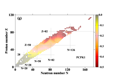


VII Conclusions
The main goal of the present study is further development of covariant energy density functionals towards more accurate description of the binding energies across the nuclear chart. It is focused on detailed analysis of the anchor based optimization approach (ABOA), its comparison with alternative global fitting protocols and on the global analysis of the errors related to the truncation of bosonic and fermionic bases in the calculation of binding energies and on the design of new fitting protocols which will allow to eliminate such errors. The main results of this study can be summarized as follows.
-
•
The detailed comparison of the anchor based optimization approach (ABOA) of global optimization of energy density functionals with fully global (FGA) and reduced global (RGA) approaches has been presented. The practical realization of each of these approaches is always a compromise between numerical accuracy in the calculation of binding energies and the number of the nuclei included into the fitting protocol. This limitation is due to the restrictions in the availability of computational power. In such a situation, an ABOA emerges as a reasonable alternative to FGA and RGA. It provides a solution which is close to that obtained in RGA but at small portion of computational time required for RGA. The correction function of Eq. (2) provides a significant push to a minimum within one to three iterations of ABOA and the use of a softer correction function of Eq. (20) guaranties the smoothness of the convergence process at further iterations.
-
•
Our analysis indicates that ten spherical anchor nuclei with experimental information on charge radii are sufficient for constraining the properties of charge radii globally in ABOA. Because of their single and doubly magic nature they are characterized by reduced theoretical uncertainties as compared with a global set of the data theoretical description of which will bring larger theoretical uncertainties. However, spin-orbit contributions to charge radii and the term of Eq. (25) have to be taken into account in the fit of the next generation of CEDFs. Note that unresolved proton radius puzzle puts a limit on the accuracy of the description of charge radii.
-
•
For the first time, the numerical errors in binding energies related to the truncation of bosonic basis have been investigated in spherical and deformed nuclei with respect of asymptotic values corresponding to the infinite basis. It was shown that these errors increase with increasing the mass of the nucleus. They also increase on transition from spherical to deformed nuclei. The dependence of these errors on the functional is weak. The truncation of bosonic basis at provides a numerical error which is better than 50 keV in all nuclei with exception of superheavy ones with and . The increase of bosonic basis to , which is easily achievable at modern computers, will reduce this error to below 10 keV for almost all nuclei of interest.
-
•
The numerical errors in binding energies related to the truncation of the fermionic basis have been systematically and globally investigated for the first time. A number of new results has been obtained. First, the way on how the calculated binding energies approach as a function of their asymptotic values depends on the type of the functional. For example, for , the absolute values of binding energy increase with increasing for the functionals which contain point coupling (PC-PK1 and DD-PC1) while it decreases for CEDFs which contain meson exchange (NL5(E), DD-ME2 and DD-MEX). Second, the convergence as a function of depends on the class of CEDF: in a given nucleus, the fastest (at lower ) approach of asymptotic values of binding energies is seen in the NLME functionals, followed by the DDME ones and the PC functionals are characterized by the slowest convergence. Third, for a given functional, the increase of either mass or the deformation of nucleus requires the increase of the size of fermionic basis for obtaining asymptotic value of binding energy.
-
•
The present paper clearly indicates the need for accounting of infinite basis corrections both for calculating the binding energies and their comparison with experimental data and for fitting of next generation of CEDFs. The current generation of CEDFs ignores these corrections. Although partially these corrections are built into the parameters of the functionals, this leads to some uncontrollable deviations in binding energies as compared with those obtained in the infinite basis. The existing prescription for finding asymptotic values of binding energy in the modest size basis which is used in non-relativistic DFTs does not provide high numerical accuracy and predictive power in the case of CDFT. An alternative procedure for finding the asymptotic values of binding energies has been suggested for the first time in the present paper (see Sec. VI). It is free from above mentioned deficiencies of non-relativistic prescription and allows better control of numerical errors in the definition of asymptotic binding energies.
The present paper clearly indicates that the binding energies of the nuclei represent the most numerically demanding type of physical observable among the ones considered at the mean field level. This is due to both their slow convergence as a function of , the request for extremely high precision in their calculation in different subfields of nuclear physics and nuclear astrophysics as well as high precision of their experimental measurements. In contrast, accurate description of other physical observables (such as deformations, moments of inertia, etc) requires substantially smaller size of fermionic basis. The present paper also indicates the need for a new generation of CEDFs which takes into account infinite basis corrections in the calculation of binding energies. The work in defining such functionals is in progress and the results of such study will be reported later.
Note that the functionals studied in the present paper are restricted to the ones defined at the mean field level. However, the results obtained here can be generalized to the approaches which include correlations beyond mean field. For example, for that the RHB approach in the anchor based optimization method has to be replaced by an appropriate beyond-mean-field method (such as a five-dimensional collective Hamiltonian Nikšić et al. (2009); Li et al. (2009); Shi et al. (2019)). This will allow to bypass the existing challenge of extreme computational cost of fitting EDFs at the beyond-mean-field level and generate such functionals. It is expected that similar to non-relativistic (see, for example, Ref. Goriely et al. (2009)) and relativistic (see Refs. Zhang et al. (2014); Yang et al. (2021)) DFT approaches this will lead to a further improvement of the description of binding energies. An alternative approach to the improvement of the description of binding energy is Bayesian Neural Network (BNN) approach in which the fluctuating part of binding energy is described with the help of statistical methods (see, for example, Refs. Utama et al. (2016); Neufcourt et al. (2018)). The BNN approaches improve the accuracy of the prediction of the binding energy at relatively modest numerical cost, provide statistical errors for predicted binding energies but do not generate a microscopic insight on the origin of the fluctuating part of binding energy which they improve.
Significant numerical cost associated with the solution of the Dirac equation in the CDFT framework calls for a search of alternative approaches to its solution. The use of Dirac oscillator basis (see Refs. Moshinsky and Szczepaniak (1989); Yang and Piekarewicz (2020)) could be one of these alternatives. This, however, requires the development of the RHB code in the Dirac oscillator basis for axially deformed nuclei. It would be also interesting to investigate whether the reduced basis method for building of efficient and accurate emulators Bonilla et al. (2022); Anderson et al. (2022) can be useful in the reduction of the computational cost. However, so far this method has been applied only to the single-particle energies and wavefunctions in spherical nuclei. Thus, the extension of this method to axially deformed nuclei and the investigations of both its accuracy in the calculation of binding energies and computational gains as compared with the method applied in the present paper are needed to establish its feasibility.
VIII ACKNOWLEDGMENTS
This material is based upon work supported by the U.S. Department of Energy, Office of Science, Office of Nuclear Physics under Award No. DE-SC0013037.
References
- Mittig et al. (2003) W. Mittig, A. Lépine-Szily, and N. A. Orr, Annu. Rev. Nucl. Sci. 47, 27 (2003).
- Dilling et al. (2018) J. Dilling, K. Blaum, M. Brodeur, and S. Eliseev, Annu. Rev. Nucl. Sci. 68, 45 (2018).
- Erler et al. (2012) J. Erler, N. Birge, M. Kortelainen, W. Nazarewicz, E. Olsen, A. M. Perhac, and M. Stoitsov, Nature 486, 509 (2012).
- Afanasjev et al. (2013) A. V. Afanasjev, S. E. Agbemava, D. Ray, and P. Ring, Phys. Lett. B 726, 680 (2013).
- Agbemava et al. (2014) S. E. Agbemava, A. V. Afanasjev, D. Ray, and P. Ring, Phys. Rev. C 89, 054320 (2014).
- Arnould et al. (2007) M. Arnould, S. Goriely, and K. Takahashi, Phys. Rep. 450, 97 (2007).
- Cowan et al. (2021) J. J. Cowan, C. Sneden, J. E. Lawler, A. Aprahamian, M. Wiescher, K. Langanke, G. Martínez-Pinedo, and F.-K. Thielemann, Rev. Mod. Phys. 93, 015002 (2021).
- Chamel and Haensel (2008) N. Chamel and P. Haensel, Living Rev. Relativity 11, 10 (2008).
- Lau et al. (2018) R. Lau, M. Beard, S. S. Gupta, A. V. Afanasjev, E. F. Brown, A. Deibel, L. R. Gasques, G. W. Hitt, W. R. Hix, L. Keek, P. Möller, A. S. P. S. Shternin, M. Wiescher, and Y. Xu, The Astrophysical J. 859, 62 (2018).
- Tondeur et al. (2000) F. Tondeur, S. Goriely, J. M. Pearson, and M. Onsi, Phys. Rev. C 62, 024308 (2000).
- Samyn et al. (2002) M. Samyn, S. Goriely, P.-H. Heenen, J. M. Pearson, and F. Tondeur, Nucl. Phys. A 700, 142 (2002).
- Goriely et al. (2013) S. Goriely, N. Chamel, and J. M. Pearson, Phys. Rev. C 88, 061302 (2013).
- Baldo et al. (2013) M. Baldo, L. M. Robledo, P. Schuck, and X. Viñas, Phys. Rev. C 87, 064305 (2013).
- Möller et al. (2016) P. Möller, A. J. Sierk, T. Ichikawa, and H. Sagawa, At. Data and Nucl. Data Tables 109, 1 (2016).
- Kortelainen et al. (2010) M. Kortelainen, T. Lesinski, J. Moré, W. Nazarewicz, J. Sarich, N. Schunck, M. V. Stoitsov, and S. Wild, Phys. Rev. C 82, 024313 (2010).
- Kortelainen et al. (2012) M. Kortelainen, J. McDonnell, W. Nazarewicz, P.-G. Reinhard, J. Sarich, N. Schunck, M. V. Stoitsov, and S. M. Wild, Phys. Rev. C 85, 024304 (2012).
- Kortelainen et al. (2014) M. Kortelainen, J. McDonnell, W. Nazarewicz, E. Olsen, P.-G. Reinhard, J. Sarich, N. Schunck, S. M. Wild, D. Davesne, J. Erler, and A. Pastore, Phys. Rev. C 89, 054314 (2014).
- Goriely et al. (2009) S. Goriely, S. Hilaire, M. Girod, and S. Péru, Phys. Rev. Lett. 102, 242501 (2009).
- Peña-Arteaga et al. (2016) D. Peña-Arteaga, S. Goriely, and N. Chamel, Eur. Phys. J. A 52, 320 (2016).
- Taninah and Afanasjev (2023) A. Taninah and A. V. Afanasjev, Phys. Rev. C 107, L041301 (2023).
- Reinhard et al. (1986) P.-G. Reinhard, M. Rufa, J. Maruhn, W. Greiner, and J. Friedrich, Z. Phys. A 323, 13 (1986).
- Vretenar et al. (2005) D. Vretenar, A. V. Afanasjev, G. A. Lalazissis, and P. Ring, Phys. Rep. 409, 101 (2005).
- Wei et al. (2020) B. Wei, Q. Zhao, Z.-H. Wang, J. Geng, B.-Y. Sun, Y.-F. Niu, and W.-H. Long, Chinese Physics C 44, 074107 (2020).
- Dobaczewski et al. (2004) J. Dobaczewski, M. V. Stoitsov, and W. Nazarewicz, AIP Conf. Proc. 726, 51 (2004).
- Pei et al. (2008) J. C. Pei, M. V. Stoitsov, G. I. Fann, W. Nazarewicz, N. Schunck, and F. R. Xu, private communication 78, 064306 (2008).
- Gonzalez-Boquera et al. (2018) C. Gonzalez-Boquera, M. Centelles, X. Vinas, and L. M. Robledo, Phys. Lett. 779, 195 (2018).
- Goriely (2023a) S. Goriely, private communication (2023a).
- Goriely et al. (2016) S. Goriely, N. Chamel, and J. M. Pearson, Phys. Rev. C 93, 034337 (2016).
- Goriely (2023b) S. Goriely, private communication (2023b).
- Zhao et al. (2010) P. W. Zhao, Z. P. Li, J. M. Yao, and J. Meng, Phys. Rev. C 82, 054319 (2010).
- Taninah et al. (2020) A. Taninah, S. E. Agbemava, A. V. Afanasjev, and P. Ring, Phys. Lett. B 800, 135065 (2020).
- Nikšić et al. (2008) T. Nikšić, D. Vretenar, and P. Ring, Phys. Rev. C 78, 034318 (2008).
- Nikšić et al. (2014) T. Nikšić, N. Paar, D. Vretenar, and P. Ring, Comp. Phys. Comm. 185, 1808 (2014).
- Gambhir et al. (1990) Y. K. Gambhir, P. Ring, and A. Thimet, Ann. Phys. (N.Y.) 198, 132 (1990).
- Boguta and Bodmer (1977) J. Boguta and R. Bodmer, Nucl. Phys. A292, 413 (1977).
- Typel and Wolter (1999) S. Typel and H. H. Wolter, Nucl. Phys. A656, 331 (1999).
- Bürvenich et al. (2002) T. Bürvenich, D. G. Madland, J. A. Maruhn, and P.-G. Reinhard, Phys. Rev. C 65, 044308 (2002).
- Lalazissis et al. (2005) G. A. Lalazissis, T. Nikšić, D. Vretenar, and P. Ring, Phys. Rev. C 71, 024312 (2005).
- Roca-Maza et al. (2011) X. Roca-Maza, X. Viñas, M. Centelles, P. Ring, and P. Schuck, Phys. Rev. C 84, 054309 (2011).
- Agbemava et al. (2019a) S. E. Agbemava, A. V. Afanasjev, and A. Taninah, Phys. Rev. C 99, 014318 (2019a).
- Wang et al. (2017) M. Wang, G. Audi, F. G. Kondev, W. Huang, S. Naimi, and X. Xu, Chinese Physics C 41, 030003 (2017).
- Press et al. (2007) W. H. Press, S. A. Teukolsky, W. T. Vetterling, and B. P. Flannery, Numerical recipies in Fortran 77. The art of scientific computing. (2d Edition, Cambridge University Press, Cambridge, 2007).
- Angeli and Marinova (2013) I. Angeli and K. P. Marinova, At. Data Nucl. Data Tables 99, 69 (2013).
- Dutra et al. (2014) M. Dutra, O. Lourenco, S. S. Avancini, B. V. Carlson, A. Delfino, D. P. Menezes, C. Providencia, S. Typel, and J. R. Stone, Phys. Rev. C 90, 055203 (2014).
- Horowitz and Piekarewicz (2012) C. J. Horowitz and J. Piekarewicz, Phys. Rev. C 86, 045503 (2012).
- Kurasawa and Suzuki (2019) H. Kurasawa and T. Suzuki, Prog. Th. Exp. Phys. 2019, 113D01 (2019).
- Friar and Negele (1975) J. L. Friar and J. W. Negele, Adv. Nucl. Phys 8, 219 (1975).
- Reinhard and Nazarewicz (2021) P.-G. Reinhard and W. Nazarewicz, Phys. Rev. C 103, 054310 (2021).
- Naito et al. (2021) T. Naito, G. Colò, H. Liang, and X. Roca-Maza, Phys. Rev. C 104, 024316 (2021).
- Zyla et al. (2020) P. A. Zyla, R. M. Barnett, J. Beringer, O. Dahl, D. A. Dwyer, D. E. Groom, C.-J. Lin, K. S. Lugovsky, E. Pianori, D. J. Robinson, C. G. Wohl, W.-M. Yao, K. Agashe, G. Aielli, B. C. Allanach, C. Amsler, M. Antonelli, E. C. Aschenauer, D. M. Asner, H. Baer, S. Banerjee, L. Baudis, C. W. Bauer, J. J. Beatty, V. I. Belousov, S. Bethke, A. Bettini, O. Biebel, K. M. Black, E. Blucher, O. Buchmuller, V. Burkert, M. A. Bychkov, R. N. Cahn, M. Carena, A. Ceccucci, A. Cerri, D. Chakraborty, R. S. Chivukula, G. Cowan, G. D’Ambrosio, T. Damour, D. de Florian, A. de Gouvêa, T. DeGrand, P. de Jong, G. Dissertori, B. A. Dobrescu, M. D’Onofrio, M. Doser, M. Drees, H. K. Dreiner, P. Eerola, U. Egede, S. Eidelman, J. Ellis, J. Erler, V. V. Ezhela, W. Fetscher, B. D. Fields, B. Foster, A. Freitas, H. Gallagher, L. Garren, H.-J. Gerber, G. Gerbier, T. G. amd Y. Gershtein, T. Gherghetta, A. A. Godizov, M. C. Gonzalez-Garcia, M. Goodman, C. Grab, A. V. Gritsan, C. Grojean, M. Grünewald, A. Gurtu, T. Gutsche, H. E. Haber, C. Hanhart, S. Hashimoto, Y. Hayato, A. Hebecker, S. Heinemeyer, B. Heltsley, J. J. Hernández-Rey, K. Hikasa, J. Hisano, A. Höcker, J. Holder, A. Holtkamp, J. Huston, T. Hyodo, K. F. Johnson, M. Kado, M. Karliner, U. F. Katz, M. Kenzie, V. A. Khoze, S. R. Klein, E. Klempt, R. V. Kowalewski, F. Krauss, M. Kreps, B. Krusche, Y. Kwon, O. Lahav, J. Laiho, L. P. Lellouch, J. Lesgourgues, A. R. Liddle, Z. Ligeti, C. Lippmann, T. M. Liss, L. Littenberg, C. Lourenco, S. B. Lugovsky, A. Lusiani, Y. Makida, F. Maltoni, T. Mannel, A. V. Manohar, W. J. Marciano, A. Masoni, J. Matthews, U.-G. Meiner, M. Mikhasenko, D. J. Miller, D. Milstead, R. E. Mitchell, K. Mönig, P. Molaro, F. Moortgat, M. Moskovic, K. Nakamura, M. Narain, P. Nason, S. Navas, M. Neubert, P. Nevski, Y. Nir, K. A. Olive, C. Patrignani, J. A. Peacock, S. T. Petcov, V. A. Petrov, A. Pich, A. Piepke, A. Pomarol, S. Profumo, A. Quadt, K. Rabbertz, J. Rademacker, G. Raffelt, H. Ramani, M. Ramsey-Musolf, B. N. Ratcliff, P. Richardson, A. Ringwald, S. Roesler, S. Rolli, A. Romaniouk, L. J. Rosenberg, J. L. Rosner, G. Rybka, M. Ryskin, R. A. Ryutin, Y. Sakai, G. P. Salam, S. Sarkar, F. Sauli, O. Schneider, K. Scholberg, A. J. Schwartz, J. Schwiening, D. Scott, V. Sharma, S. R. Sharpe, T. Shutt, M. Silari, T. Sjöstrand, P. Skands, T. Skwarnicki, G. F. Smoot, A. Soffer, M. S. S. S. Spanier, C. Spiering, A. Stahl, S. L. Stone, Y. Sumino, T. Sumiyoshi, M. J. Syphers, F. Takahashi, M. Tanabashi, J. Tanaka, M. Taŝevský, K. Terashi, J. Terning, U. Thoma, R. S. Thorne, L. Tiator, M. Titov, N. P. Tkachenko, D. R. Tovey, K. Trabelsi, P. Urquijo, G. Valencia, R. V. de Water, N. Varelas, G. Venanzoni, L. Verde, M. G. Vincter, P. Vogel, W. Vogelsang, A. Vogt, V. Vorobyev, S. P. Wakely, W. Walkowiak, C. W. Walter, D. Wands, M. O. Wascko, D. H. Weinberg, E. J. Weinberg, M. White, L. R. Wiencke, S. Willocq, C. L. Woody, R. L. Workman, M. Yokoyama, R. Yoshida, G. Zanderighi, G. P. Zeller, O. V. Zenin, R.-Y. Zhu, and S.-L. Zhu, Prog. Theor. Part. Phys. 083C01 (2020).
- Sick (2018) I. Sick, Atoms 6, 1 (2018).
- Gao and Vanderhaeghen (2022) H. Gao and M. Vanderhaeghen, Rev. Mod. Phys. 94, 015002 (2022).
- Perera et al. (2021) U. C. Perera, A. V. Afanasjev, and P. Ring, Phys. Rev. C 104, 064313 (2021).
- Campbell et al. (2016) P. Campbell, I. Moore, and M. Pearson, Prog. Part. Nucl. Phys. 86, 127 (2016).
- Naito et al. (2022) T. Naito, T. Oishi, H. Sagawa, and Z. Wang, Phys. Rev. C 107, 054307 (2022).
- Perera and Afanasjev (2023) U. C. Perera and A. V. Afanasjev, Phys. Rev. C 107, 064321 (2023).
- Bonneau et al. (2007) L. Bonneau, P. Quentin, and P. Möller, Phys. Rev. C 76, 024320 (2007).
- Litvinova and Afanasjev (2011) E. V. Litvinova and A. V. Afanasjev, Phys. Rev. C 84, 014305 (2011).
- Dobaczewski et al. (2015) J. Dobaczewski, A. V. Afanasjev, M. Bender, L. M. Robledo, and Y. Shi, Nucl. Phys. A 944, 388 (2015).
- Lalazissis et al. (1999) G. A. Lalazissis, S. Raman, and P. Ring, At. Data Nucl. Data Table 71, 1 (1999).
- Geng et al. (2005) L. Geng, H. Toki, and J. Meng, Prog. Theor. Phys. 113, 785 (2005).
- Reinhard and Agrawal (2011) P.-G. Reinhard and B. K. Agrawal, Int. Jour. Mod. Phys. E20, 1379 (2011).
- Zhang et al. (2014) Q. S. Zhang, Z. M. Niu, Z. P. Li, J. M. Yao, and J. Meng, Frontiers of Physics 9, 529 (2014).
- Lu et al. (2015) K. Q. Lu, Z. X. Li, Z. P. Li, J. M. Yao, and J. Meng, Phys. Rev. C 91, 027304 (2015).
- Yang et al. (2021) Y. L. Yang, Y. K. Wang, P. W. Zhao, and Z. P. Li, Phys. Rev. C 104, 054312 (2021).
- Agbemava et al. (2019b) S. E. Agbemava, A. V. Afanasjev, A. Taninah, and A. Gyawali, Phys. Rev. C 99, 034316 (2019b).
- Reinhard (1989) P.-G. Reinhard, Rep. Prog. Phys. 52, 439 (1989).
- Hilaire and Girod (2007) S. Hilaire and M. Girod, Eur. Phys. J. 33, 237 (2007).
- Kortelainen (2023) M. Kortelainen, private communication (2023).
- Nikšić et al. (2009) T. Nikšić, Z. P. Li, D. Vretenar, L. Próchniak, J. Meng, and P. Ring, Phys. Rev. C 79, 034303 (2009).
- Li et al. (2009) Z. P. Li, T. Nikšić, D. Vretenar, J. Meng, G. A. Lalazissis, and P. Ring, Phys. Rev. C 79, 054301 (2009).
- Shi et al. (2019) Z. Shi, A. V. Afanasjev, Z. P. Li, and J. Meng, Phys. Rev. C 99, 064316 (2019).
- Utama et al. (2016) R. Utama, J. Piekarewicz, and H. B. Prosper, Phys. Rev. C 93, 014311 (2016).
- Neufcourt et al. (2018) L. Neufcourt, Y. Cao, W. Nazarewicz, and F. Viens, Phys. Rev. C 98, 034318 (2018).
- Moshinsky and Szczepaniak (1989) M. Moshinsky and A. Szczepaniak, Journal of Physics A: Mathematical and General 22, L817 (1989).
- Yang and Piekarewicz (2020) J. Yang and J. Piekarewicz, Phys. Rev. C 102, 054308 (2020).
- Bonilla et al. (2022) E. Bonilla, P. Giuliani, K. Godbey, and D. Lee, Phys. Rev. C 106, 054322 (2022).
- Anderson et al. (2022) A. L. Anderson, G. L. O’Donnell, and J. Piekarewicz, Phys. Rev. C 106, L031302 (2022).