Towards a Novel Perspective on Adversarial Examples Driven by Frequency
Abstract
Enhancing our understanding of adversarial examples is crucial for the secure application of machine learning models in real-world scenarios. A prevalent method for analyzing adversarial examples is through a frequency-based approach. However, existing research indicates that attacks designed to exploit low-frequency or high-frequency information can enhance attack performance, leading to an unclear relationship between adversarial perturbations and different frequency components. In this paper, we seek to demystify this relationship by exploring the characteristics of adversarial perturbations within the frequency domain. We employ wavelet packet decomposition for detailed frequency analysis of adversarial examples and conduct statistical examinations across various frequency bands. Intriguingly, our findings indicate that significant adversarial perturbations are present within the high-frequency components of low-frequency bands. Drawing on this insight, we propose a black-box adversarial attack algorithm based on combining different frequency bands. Experiments conducted on multiple datasets and models demonstrate that combining low-frequency bands and high-frequency components of low-frequency bands can significantly enhance attack efficiency. The average attack success rate reaches 99%, surpassing attacks that utilize a single frequency segment. Additionally, we introduce the normalized disturbance visibility index as a solution to the limitations of norm in assessing continuous and discrete perturbations111Our code will be released soon..
1 Introduction
With the advent of deep learning, neural network models have demonstrated groundbreaking performance across a variety of computer vision tasks Aceto et al. (2021); Menghani (2023). However, the emergence of adversarial examples has exposed vulnerabilities in deep neural networks (DNNs) Goodfellow et al. (2014); Van Le et al. (2023). These maliciously crafted adversarial examples are designed to induce misclassification in a target model by introducing human-imperceptible perturbations to clean examples. Such vulnerabilities impede the deployment of DNNs in security-sensitive domains.
Enhancing our comprehension of adversarial examples is pivotal for the development of trustworthy AI. A common method for examining adversarial examples is the signal-processing perspective of frequencies Yin et al. (2019); Wang et al. (2020a); Lorenz et al. (2021); Deng and Karam (2022); Qian et al. (2023). Typically, low-frequency components of images hold primary information, such as smooth backgrounds or uniform color areas, while high-frequency is associated with rapid changes in texture, edges, or noise.
However, adversarial examples in frequency domains remain a subject of debate Han et al. (2023). Goodfellow et al.Goodfellow et al. (2014) highlight the sensitivity of DNN activations to the high-frequency elements within images. Subsequent studies Wang et al. (2020b); Yin et al. (2019) have underscored the impact of high-frequency signals on DNN predictions, while other research Guo et al. (2018); Sharma et al. (2019) posits that low-frequency perturbations can also effectively compromise models. Furthermore, Geirhos et al.Geirhos et al. (2018) discover that DNNs trained on ImageNet are highly biased towards the texture (high-frequency) and shape (low-frequency) aspects of objects. Recent research reveals that adversarial examples are neither in high-frequency nor low-frequency components Maiya et al. (2021); Qian et al. (2023). Consequently, the relationship between adversarial perturbations and frequency components remains uncertain, inviting further exploration in the frequency domain.
In this paper, we explore the relationship between adversarial perturbations and frequency components in the frequency domain. We utilize wavelet packet decomposition (WPD) to analyse adversarial perturbations, which provide a more nuanced analysis of local frequency characteristics than discrete cosine transform (DCT) or traditional wavelet analysis. Our analysis, supported by statistical data across different frequency bands, reveals a counterintuitive pattern: significant adversarial perturbations are predominantly present in the high-frequency components of low-frequency bands. Based on these findings, we propose a black-box adversarial attack algorithm that can add perturbations to any combinations of frequency bands separately. Experiments on three mainstream datasets and three models show that combining low-frequency bands and high-frequency components of low-frequency bands can effectively attack deep learning models, surpassing attacks that utilize a single frequency band. Moreover, we find there are limitations of norm in evaluating continuous and discrete perturbations when assessing the imperceptibility of adversarial examples. To overcome this, we introduce the normalized disturbance visibility (NDV) index, which normalizes the norm for a more accurate evaluation that aligns more closely with human perception.
The main contributions can be summarized as follows:
-
•
Our research into the relationship between adversarial perturbations and frequency components in the frequency domain has uncovered a counterintuitive phenomenon: significant adversarial perturbations predominantly reside within the high-frequency parts of low-frequency bands. This finding has the potential to deepen our understanding of adversarial examples and to guide the design of adversarial attack and defense strategies.
-
•
We propose a novel black-box adversarial attack algorithm leveraging frequency decomposition. Experiment results on three datasets (CIFAR-10, CIFAR-100 and ImageNet) and three models (ResNet-50, DenseNet-121 and InceptionV3) show that the strategy of combining low-frequency bands and high-frequency components of low-frequency significantly improves attack efficiency, with an average attack success rate of 99%, outperforming approaches that utilize a single-frequency band.
-
•
We introduce the NDV to address the issue of norm in assessing continuous and discrete perturbations, which provides a more comprehensive measure that aligns closely with human visual perception.
2 Related Works
2.1 Adversarial Example
The notion of adversarial examples is initially introduced by Szegedy et al. Goodfellow et al. (2014). They leverage gradient information to ingeniously engineer minor modifications in images. These alterations, generally imperceptible to the human eye, are sufficient to mislead classification algorithms into incorrect predictions. According to knowledge of the target model, adversarial attacks can be classified as white-box attacks or black-box attacks. In white-box attack scenarios, attackers have access to gradients of models, enabling them to generate highly precise perturbations Athalye et al. (2018); Carlini and Wagner (2017); Kurakin et al. (2018); Madry et al. (2017). Black-box attacks are broadly categorized into query-based and transfer-based types. Query-based attacks leverage feedback from model queries to craft adversarial examples Chen et al. (2020); Cheng et al. (2018); Tu et al. (2019); Guo et al. (2019); Andriushchenko et al. (2020). Brendel et al. Brendel et al. (2017) pioneered the decision-based black-box attack Cheng et al. Chen et al. (2017) introducing a zero-order optimization technique through gradient estimation. Conversely, transfer-based attacks involve creating adversarial examples on substitute models and transferring them to the target model Cheng et al. (2019); Huang and Zhang (2019); Huang et al. (2019); Shi et al. (2019). However, compared to query-based attacks, transfer-based attacks are often constrained by challenges in building effective substitute models and their relatively lower rates of attack success.
2.2 Frequency for Adversarial Example.
Numerous studies Tsuzuku and Sato (2019); Guo et al. (2018); Sharma et al. (2019); Lorenz et al. (2021); Wang et al. (2020a) have analyzed DNNs from a frequency domain perspective. Tsuzuku & Sato Tsuzuku and Sato (2019) pioneer the frequency framework by investigating the sensitivity of DNNs to different Fourier bases. Building on this, Guo et al. Guo et al. (2018) design pioneering adversarial attacks targeting low-frequency components. This approach is corroborated by Sharma et al. Sharma et al. (2019), who demonstrate the efficacy of such attacks against models fortified with adversarial defenses. Concurrently, efforts by Lorenz et al. Lorenz et al. (2021) and Wang et al. Wang et al. (2020a) have propelled forward the detection of adversarial examples, utilizing frequency domain strategies during model training.
Additionally, some studies Wang et al. (2020b, c) have demonstrated that DNNs are more vulnerable to high-frequency components, resulting in models with low robustness. It is also the principal rationale for preprocessing-based defence methods. Confusingly, these findings are contradictory to the idea of low-frequency adversarial attacksIlyas et al. (2019); Sharma et al. (2019). To explain the performance of adversarial examples in frequency domains, Maiya et al. Maiya et al. (2021) argue that adversarial examples are neither high-frequency nor low-frequency and are only relevant to the dataset. In addition, Abello et al. Abello et al. (2021) and Caro et al. Caro et al. (2020) argue that the frequency of images is an intrinsic characteristic of the robustness of models. Recent studies Qian et al. (2023) have shown that attacks targeting both low-frequency and high-frequency information can enhance attack performance, indicating that the relationship between learning behavior and different frequency information remains to be explored.
3 Frequency Analysis of Adversarial Perturbations
In this section, we introduce the steps to analyze adversarial perturbation in the frequency domain, including 1) adversarial perturbation generation, 2) frequency decomposition, and 3) frequency analysis.
3.1 Adversarial Perturbation Generation
To examine the characteristics of adversarial perturbations, we first generate these disruptive inputs. FGSM Goodfellow et al. (2014) and PGD Madry et al. (2017) are prominent techniques for creating adversarial examples, commonly used to assess the robustness of deep learning models. Consequently, we employ these two methods for generating adversarial examples. To be specific, given some images , whose corresponding labels . The adversarial example generation formula for FGSM is as Eq.1:
| (1) |
where, is a parameter that controls the magnitude of the perturbation. represents the sign of the gradient of the loss function with respect to the input image, which determines the direction of the perturbation. PGD generates an adversarial example by performing the iterative update with Eq.2:
| (2) |
where is the step size at iteration , is adversarial example at iteration and clips the input to the ball of . is the gradient at iteration .

3.2 Frequency Decomposition
Wavelet packet decomposition (WPD) employs multi-level data decomposition to extract detailed and approximate information from signals. This method iteratively decomposes all frequency components, enabling a comprehensive frequency stratification. This contrasts traditional wavelet analysis, which primarily decomposes only the low-frequency parts. Through WPD, an image is separated into a series of frequency bands, each capturing distinct components of the image. The low-frequency band typically encapsulates fundamental image characteristics, such as overall luminosity, color, and structural composition. In contrast, high-frequency bands contain secondary image information like edges and textures Prasad and Iyengar (2020).
We apply WPD for frequency decomposition. The wavelet packet comprises a set of functions that include the scaling function and the wavelet function , as depicted in Eq.3:
| (3) |
where is low-pass filter, is high-pass filter. The decomposition process of WPD can be expressed as Eq.4:
| (4) |
where and are wavelet packet coefficients obtained by the decomposition of . So we decompose , into frequency domains by Eq.4, and we get different wavelet packet coefficients and respectively. The wavelet packet coefficient determines the frequency band, so we think of them as the frequency band.
For ease of description, high-frequency components are denoted as , and low-frequency components as . WPD follows a binary decomposition process, resulting in a tree structure as illustrated in Figure 1. After decompositions, frequency bands are obtained. These decomposed frequency bands can be reassembled using Eq.5:
| (5) |
3.3 Frequency Analysis
We employ WPD to dissect both normal images and their corresponding adversarial examples into a series of frequency bands. This approach allows us to compute the cosine similarity between adversarial and clean samples within each band, thereby analyzing the spread of adversarial perturbations across different frequency segments. For an image and its adversarial counterpart , we apply WPD to decompose into frequency bands and into . Subsequently, we calculate their cosine similarity as per Eq.6.
| (6) |
The experimental results are depicted in Figure 2, demonstrating that lower similarity corresponds to greater perturbations. Initially, after the first decomposition ( layer), adversarial perturbations predominantly appear in the high-frequency component , aligning with previous research that identifies adversarial perturbations as high-frequency components Wang et al. (2020b, c). Interestingly, after the second decomposition ( layer), these perturbations concentrate more in the band, with further decrease in similarity observed in the band after the third decomposition ( layer). The band which decomposes from the low-frequency band originating from the high band , also exhibits reduced similarity. This pattern suggests that adversarial perturbations are prevalent in higher-frequency components within low-frequency bands. Furthermore, at the third decomposition level, the band with the third-lowest similarity is the highest frequency band , indicating that adversarial perturbations, although inherently high-frequency, depend on the low-frequency information from their preceding levels. For more details, see Section 6.2.

4 Black-box Adversarial Attack Based on Frequency Decomposition
In this section, we introduce a black-box adversarial attack methodology grounded in frequency decomposition. The framework of our attack is depicted in Figure 3, accompanied by the corresponding pseudo-code in Algorithm 1. The core components include frequency band selection and attack implementation.

4.1 Frequency Selection
As discussed in Section 3.3, our experimental findings indicate that adversarial perturbations predominantly appear in specific high-frequency bands originating from low-frequency bands. Particularly at the layer, the and bands, decompose from and respectively, exhibit lower similarity. This indicates a higher concentration of adversarial perturbations in these bands. The lowest frequency band encompasses crucial image information like color, brightness, and structural luminance, contrasting with the other seven bands, which are mainly associated with edges and textures. This difference implies that the band holds more substantial information, as illustrated in Figure 1, where areas with lower information content are in black (value of 0). Consequently, we combine the low-frequency band and the high-frequency components of low-frequency bands as the main search area. The ablation experiments for these three frequency bands are detailed in Section 5.
4.2 Attack Implementation
Inspired by the work of Guo et al Guo et al. (2019), we propose a black-box adversarial attack. This approach includes orthogonal direction vector selection, iterative approach and perturbation limitations.
Orthogonal direction vector selection. To effectively reduce the number of searches, verifying that all vectors in frequency bands are orthonormal is essential. Decompose space into wavelet subspace , such as . We further orthogonal decompose the subspace into . According to wavelet theory, wavelet packet decompositions satisfy Eq.7. Therefore, after three times decomposition, we yield , which are orthogonal to each other. So the frequency band are mutually orthogonal. The , which we choose from without repeat, is also orthogonal, where is the orthogonal direction vector specified in this paper.
| (7) |
Iterative approach. Pick band from according to the initialization probability . Then, initialize a matrix of size with the value for random points and for the rest. No point in will be selected twice. Therefore, each is an orthogonal vector we picked. We add perturbations to the frequency band through . Since belongs to and belongs to , our perturbations are added to . We can reconstruct the perturbed to image by Eq.5. Input into the model for a query. These modifications may likely lower the . And we get the in the current search. Then, we update the probability based on the and choose another orthogonal vector for the subsequent iteration. To maintain the query efficiency, we ensure that no two directions cancel each other out.
Perturbation limitations. We can control perturbations by adjusting the step size and (parameter determines the generation of ). In each iteration, points are added, subtracted, or discarded (if the output probability is not reduced in either direction). Suppose that represents the symbol of the search direction chosen at step . Therefore, perturbations after steps in frequency domains satisfy Eq.8. Our analysis highlights a critical trade-off: (1) for query-limited situations, raising and can increase the attack success rate while decreasing the number of inquiries. (2) Reduce and to produce imperceptible perturbations in perturbation-limited situations.
| (8) |

| Datasets | Models | Attacks | layer | layer | layer | |||||||||||
| a | d | aa | da | ad | dd | aaa | daa | ada | dda | aad | dad | add | ddd | |||
| CIRAR10 | Den | FGSM | 0.9986 | 0.7915 | 0.9992 | 0.6879 | 0.9367 | 0.8249 | 0.9995 | 0.6778 | 0.9133 | 0.8574 | 0.9763 | 0.6906 | 0.9483 | 0.7659 |
| PGD | 0.9991 | 0.8563 | 0.9994 | 0.7649 | 0.9608 | 0.8837 | 0.9996 | 0.7525 | 0.9456 | 0.9069 | 0.9849 | 0.7699 | 0.9680 | 0.8394 | ||
| R50 | FGSM | 0.9986 | 0.7987 | 0.9991 | 0.6984 | 0.9366 | 0.8301 | 0.9994 | 0.6905 | 0.9139 | 0.8608 | 0.9756 | 0.7002 | 0.9477 | 0.7754 | |
| PGD | 0.9992 | 0.8646 | 0.9995 | 0.7776 | 0.9621 | 0.8904 | 0.9996 | 0.7645 | 0.9479 | 0.9122 | 0.9853 | 0.7830 | 0.9687 | 0.8488 | ||
| V3 | FGSM | 0.9990 | 0.7387 | 0.9995 | 0.5610 | 0.9457 | 0.8271 | 0.9997 | 0.4965 | 0.9206 | 0.8641 | 0.9831 | 0.6076 | 0.9583 | 0.7639 | |
| PGD | 0.9994 | 0.8528 | 0.9997 | 0.7174 | 0.9694 | 0.9043 | 0.9998 | 0.6714 | 0.9559 | 0.9256 | 0.9897 | 0.7475 | 0.9758 | 0.8627 | ||
| Vgg | FGSM | 0.9989 | 0.7591 | 0.9994 | 0.6161 | 0.9405 | 0.8192 | 0.9996 | 0.5751 | 0.9139 | 0.8535 | 0.9803 | 0.6426 | 0.9539 | 0.7594 | |
| PGD | 0.9994 | 0.8472 | 0.9996 | 0.7255 | 0.9656 | 0.8915 | 0.9998 | 0.6868 | 0.9494 | 0.9128 | 0.9887 | 0.7494 | 0.9733 | 0.8498 | ||
| CIRAR100 | Den | FGSM | 0.9985 | 0.7884 | 0.9990 | 0.6955 | 0.9280 | 0.8172 | 0.9993 | 0.6780 | 0.8994 | 0.8432 | 0.9733 | 0.7031 | 0.9416 | 0.7667 |
| PGD | 0.9990 | 0.8504 | 0.9993 | 0.7643 | 0.9547 | 0.8766 | 0.9995 | 0.7471 | 0.9364 | 0.8976 | 0.9828 | 0.7721 | 0.9629 | 0.8342 | ||
| R50 | FGSM | 0.9984 | 0.8084 | 0.9990 | 0.7261 | 0.9238 | 0.8319 | 0.9992 | 0.7070 | 0.8937 | 0.8509 | 0.9727 | 0.7350 | 0.9387 | 0.7926 | |
| PGD | 0.9990 | 0.8601 | 0.9993 | 0.7866 | 0.9518 | 0.8806 | 0.9995 | 0.7706 | 0.9311 | 0.8970 | 0.9825 | 0.7935 | 0.9616 | 0.8467 | ||
| V3 | FGSM | 0.9988 | 0.7468 | 0.9993 | 0.5843 | 0.9445 | 0.8305 | 0.9996 | 0.5255 | 0.9220 | 0.8671 | 0.9795 | 0.6278 | 0.9549 | 0.7675 | |
| PGD | 0.9992 | 0.8459 | 0.9995 | 0.7123 | 0.9632 | 0.8948 | 0.9997 | 0.6658 | 0.9500 | 0.9171 | 0.9856 | 0.7410 | 0.9690 | 0.8498 | ||
| Vgg | FGSM | 0.9988 | 0.7532 | 0.9993 | 0.6120 | 0.9396 | 0.8146 | 0.9996 | 0.5681 | 0.9142 | 0.8503 | 0.9782 | 0.6394 | 0.9515 | 0.7517 | |
| PGD | 0.9994 | 0.8506 | 0.9996 | 0.7321 | 0.9671 | 0.8932 | 0.9998 | 0.6940 | 0.9528 | 0.9154 | 0.9884 | 0.7549 | 0.9734 | 0.8492 | ||
| ImageNet | Den | FGSM | 0.9983 | 0.6885 | 0.9989 | 0.5980 | 0.8451 | 0.7216 | 0.9993 | 0.5766 | 0.8042 | 0.7549 | 0.9272 | 0.6079 | 0.8603 | 0.6603 |
| PGD | 0.9993 | 0.7657 | 0.9996 | 0.6694 | 0.9215 | 0.8026 | 0.9997 | 0.6426 | 0.8869 | 0.8347 | 0.9721 | 0.6836 | 0.9351 | 0.7421 | ||
| R50 | FGSM | 0.9985 | 0.6625 | 0.9991 | 0.5821 | 0.8452 | 0.6907 | 0.9994 | 0.5690 | 0.7918 | 0.7251 | 0.9407 | 0.5856 | 0.8691 | 0.6290 | |
| PGD | 0.9994 | 0.7655 | 0.9996 | 0.6750 | 0.9239 | 0.7995 | 0.9997 | 0.6525 | 0.8884 | 0.8317 | 0.9748 | 0.6861 | 0.9387 | 0.7394 | ||
| V3 | FGSM | 0.9982 | 0.6927 | 0.9988 | 0.6101 | 0.8314 | 0.7197 | 0.9993 | 0.5874 | 0.7896 | 0.7441 | 0.9142 | 0.6188 | 0.8447 | 0.6644 | |
| PGD | 0.9993 | 0.7665 | 0.9996 | 0.6699 | 0.9119 | 0.8016 | 0.9997 | 0.6407 | 0.8769 | 0.8282 | 0.9662 | 0.6837 | 0.9238 | 0.7429 | ||
| Vgg | FGSM | 0.9983 | 0.6685 | 0.9989 | 0.5788 | 0.8486 | 0.7022 | 0.9993 | 0.5551 | 0.8016 | 0.7342 | 0.9368 | 0.5916 | 0.8682 | 0.6430 | |
| PGD | 0.9993 | 0.7608 | 0.9996 | 0.6661 | 0.9222 | 0.7994 | 0.9997 | 0.6392 | 0.8869 | 0.8305 | 0.9732 | 0.6817 | 0.9364 | 0.7412 | ||
| AVE | 0.9989 | 0.7826 | 0.9993 | 0.6755 | 0.9267 | 0.8228 | 0.9996 | 0.6473 | 0.8994 | 0.8506 | 0.9713 | 0.6915 | 0.9385 | 0.7702 | ||
5 Normalized Disturbance Visibility Index
The norm is widely used to measure the imperceptibility by quantifying the perturbation magnitude between original and adversarial examples. It gauges the overall effect of the adversarial perturbation on the original input, helping to ensure that the resulting adversarial samples remain either imperceptible or minimally perceptible to human observers. However, our findings suggest that the norm might fall short in accurately evaluating adversarial examples that comprise continuous and discrete perturbations, as shown in Figure 4. Even with an equivalent norm, perturbations from patch attacks (see Figure 4(c)) tend to be more discernible to the human eye.
Normalized Disturbance Visibility Index. To align more closely with human perceptual observations, we refine the norm into a more sophisticated metric, the Normalized Disturbance Visibility (NDV) Index. For a pure sample and its corresponding adversarial example , the NDV is computed as outlined in Eq.9. This index modifies the norm by dividing it by the number of points affected by the perturbation. To circumvent issues of non-differentiability, we introduce a small constant in the denominator. Moreover, for standardizing the scale measurements, we multiply the final value by a constant (defaulted to 1000). The NDV values, akin to the norm, convey the magnitude of perturbations: a larger value indicates more significant perturbations, while a smaller value denotes less pronounced perturbations.
| (9) |
6 Experiments
6.1 Datasets and Models
Following the previous study Guo et al. (2019), we randomly pick 1000 images from validation sets of CIFAR-10 Krizhevsky et al. (2009), CIFAR-100 Krizhevsky et al. (2009) and ImageNet-1K Russakovsky et al. (2015), respectively, as test dataset. These samples are initially correctly classified to avoid artificially boosting the success rate. In CIFAR-10 and CIFAR-100, we are standardized training the models of ResNet-50, VGG16 and InceptionV3 following the steps outlined in He et al. (2016); Huang et al. (2017); Szegedy et al. (2016). On ImageNet-1K, we choose pre-trained models of ResNet-50, VGG16, InceptionV3 and DenseNet-121 from Pytorch Paszke et al. (2019).
6.2 Experiments on Adversarial Perturbations in Frequency
We analyze the distribution of adversarial perturbations in the frequency domain using a combination of three datasets (ImageNet-1K, CIFAR-10, and CIFAR-100), four models (VGG16, ResNet-50, DenseNet-121, and InceptionV3), and two attacks (FGSM and PGD). By computing the cosine similarity between adversarial and pure examples, we assess the distribution of adversarial perturbations across various frequency bands, as detailed in Table 1. The results reveal a consistent trend across diverse datasets, models, and attack strategies: the cosine similarity between normal and adversarial samples is markedly lower within , and frequency bands. This trend suggests that adversarial perturbations predominantly occur in high-frequency bands of low-frequency bands. Moreover, although perturbations are distinctly observed in certain frequency bands, the complete separation of adversarial perturbations remains elusive, both through the use of different wavelet functions and further decomposition of the third-layer frequency band. This suggests that current wavelet functions are inadequate for the separation of adversarial perturbations. Designing new wavelet functions specifically for the characteristics of adversarial perturbations might facilitate a more complete separation of these perturbations.
6.3 Evaluations of Our Proposed Method
In this section, we evaluate our method on multiple datasets and models and also compare it with state-of-the-art approaches. All experiments are untargeted attacks. For performance evaluation and comparison, we employ the Attack Success Rate (ASR) and six other distinct metrics. These include the Average Number of Queries (ANQ), Median Number of Queries (MNQ), norm, norm, Structural Similarity Index (SSIM), and our proposed NDV.
Evaluations on Different Models. We evaluate our proposed attack method on DenseNet121, ResNet50 and InceptionV3 using CIFAR-10 and CIFAR-100 datasets. As shown in Table 2, the results demonstrate that our method can efficiently attack various models, with ASR exceeding 98%. In particular, for the InceptionV3 model, an average of only a few dozen queries is needed for a successful attack.
| Models | ASR | ANQ | MNQ | SSIM | NDV | |||
|---|---|---|---|---|---|---|---|---|
| C10 | Den | 0.948 | 219.63 | 176 | 2.27 | 0.18 | 0.99 | 0.744 |
| R50 | 0.995 | 235.07 | 180 | 2.35 | 0.19 | 0.99 | 0.760 | |
| V3 | 1.000 | 80.14 | 54 | 1.23 | 0.13 | 0.99 | 0.403 | |
| C100 | Den | 0.997 | 179.49 | 137 | 2.06 | 0.18 | 0.99 | 0.676 |
| R50 | 0.998 | 216.28 | 154 | 2.24 | 0.19 | 0.99 | 0.736 | |
| V3 | 0.995 | 59.22 | 42 | 1.12 | 0.12 | 0.99 | 0.372 |
| Methods | Models | ASR | ANQ | MNQ | SSIM | NDV | ||
|---|---|---|---|---|---|---|---|---|
| Boundary | Den | 1.000 | 9077.00 | 5700 | 13.98 | 0.11 | 0.78 | 0.092 |
| R50 | 1.000 | 9820.06 | 7922 | 13.98 | 0.11 | 0.79 | 0.092 | |
| GeoDA | Den | 1.000 | 3350.96 | 4078 | 32.99 | 0.35 | 0.87 | 0.223 |
| R50 | 1.000 | 3213.37 | 3329 | 30.98 | 0.33 | 0.87 | 0.210 | |
| SimBA | Den | 0.986 | 508.02 | 341 | 4.59 | 0.05 | 0.99 | 0.031 |
| R50 | 0.984 | 560.02 | 349 | 4.65 | 0.05 | 0.99 | 0.031 | |
| Square | Den | 0.888 | 365.91 | 86 | 13.66 | 0.71 | 0.94 | 0.153 |
| R50 | 0.886 | 429.49 | 71 | 13.64 | 0.71 | 0.94 | 0.155 | |
| Attack | Den | 0.879 | 834.93 | 613 | 10.84 | 0.05 | 0.94 | 0.072 |
| R50 | 0.927 | 663.39 | 409 | 11.39 | 0.05 | 0.94 | 0.076 | |
| Ours | Den | 0.995 | 380.58 | 183 | 12.53 | 0.29 | 0.96 | 0.084 |
| R50 | 0.992 | 426.11 | 184 | 12.85 | 0.29 | 0.96 | 0.086 |
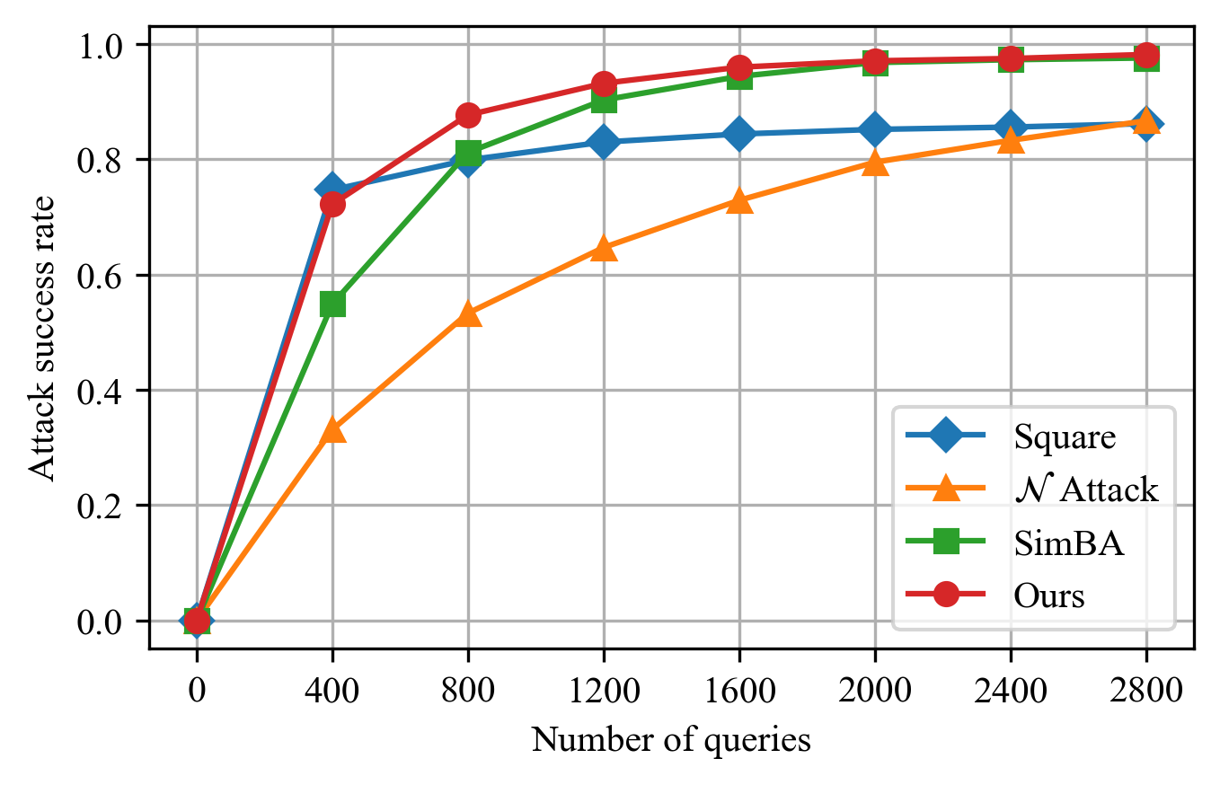
Comparisons with State-of-the-Art Methods. We compare our attack with state-of-the-art black-box attack algorithms, including Boundary Attack Brendel et al. (2017), GeoDA attack Rahmati et al. (2020), Square Attack Andriushchenko et al. (2020), Attack Li et al. (2019), SimBA Guo et al. (2019). As shown in Table 3, our attack achieves a fine balance between attack success, imperceptibility, and query efficiency, marking it as a superior strategy for adversarial attacks in practical applications. Figure 5 illustrates the relationship between the number of queries and attack success rate, with results indicating that our method can achieve a high success rate with fewer queries.

Ablation Studies. We investigate the contributions of three selected frequency bands—denoted as A (), B (), and C ()—in generating adversarial perturbations, with the results detailed in Table 4. Band A demonstrates the highest individual ASR, underscoring its significant role in adversarial attacks, aligning with the studies of Wang et al Wang et al. (2020c). Combinations AB and AC yield higher ASR than each band individually, suggesting that the integration of bands B and C enhances attack efficacy. Notably, the ABC combination achieves the highest ASR, outperforming all single and dual-band combinations, while other evaluated metrics remain relatively unchanged.
| ASR | ANQ | MNQ | SSIM | NDV | |||
| A | 0.955 | 181.74 | 153 | 1.79 | 0.12 | 0.99 | 0.59 |
| B | 0.637 | 263.20 | 251 | 2.20 | 0.14 | 0.99 | 0.72 |
| C | 0.822 | 219.00 | 192 | 1.94 | 0.14 | 0.99 | 0.63 |
| AB | 0.982 | 271.47 | 216 | 2.66 | 0.21 | 0.99 | 0.87 |
| AC | 0.987 | 216.16 | 166 | 2.27 | 0.17 | 0.99 | 0.74 |
| BC | 0.907 | 264.38 | 198 | 2.42 | 0.20 | 0.99 | 0.79 |
| ABC | 0.995 | 235.07 | 180 | 2.35 | 0.19 | 0.99 | 0.76 |
6.4 Comparisons of and NDV
To enhance the comparative analysis between NDV and the norm, we select three sets of examples, as demonstrated in Figure 6. The first column displays the clean samples, while the second and third columns showcase adversarial examples created by our proposed method and the square attack method, respectively. The outcomes reveal that, despite nearly identical norms, the adversarial examples produced by the square attack exhibit more noticeable color variations and artifacts, thus making them more discernible to the human eye. In contrast, the changes in NDV values more accurately reflect the perceptual sensitivity of human observers.

7 Conclusion
Our investigation into the frequency attributes of adversarial perturbations has provided new insights into the comprehension of adversarial examples. The result of wavelet packet decomposition reveals that most perturbations are present within the lower-frequency components of high-frequency bands, thus refuting the simplistic dichotomy of perturbations as merely low or high-frequency. Based on these insights, we propose a black-box adversarial attack algorithm that strategically employs combinations of different frequency bands to enhance attack efficacy. This innovative approach not only broadens the understanding of frequency-based adversarial strategies but also demonstrates higher efficiency compared to attacks that do not consider specific frequency components. Furthermore, to address the inadequacies of the norm for evaluating perturbations, we propose the NDV, which provides a more comprehensive measure that aligns closely with human visual perception. Our findings emphasize the value of a frequency-centric perspective in developing secure machine learning frameworks and advancing defenses against adversarial examples.
References
- Abello et al. [2021] Antonio A Abello, Roberto Hirata, and Zhangyang Wang. Dissecting the high-frequency bias in convolutional neural networks. In Proceedings of the IEEE/CVF Conference on Computer Vision and Pattern Recognition, pages 863–871, 2021.
- Aceto et al. [2021] Giuseppe Aceto, Domenico Ciuonzo, Antonio Montieri, and Antonio Pescapé. Distiller: Encrypted traffic classification via multimodal multitask deep learning. Journal of Network and Computer Applications, 183:102985, 2021.
- Andriushchenko et al. [2020] Maksym Andriushchenko, Francesco Croce, Nicolas Flammarion, and Matthias Hein. Square attack: a query-efficient black-box adversarial attack via random search. In European Conference on Computer Vision, pages 484–501. Springer, 2020.
- Athalye et al. [2018] Anish Athalye, Logan Engstrom, Andrew Ilyas, and Kevin Kwok. Synthesizing robust adversarial examples. In International conference on machine learning, pages 284–293. PMLR, 2018.
- Brendel et al. [2017] Wieland Brendel, Jonas Rauber, and Matthias Bethge. Decision-based adversarial attacks: Reliable attacks against black-box machine learning models. arXiv preprint arXiv:1712.04248, 2017.
- Carlini and Wagner [2017] Nicholas Carlini and David Wagner. Towards evaluating the robustness of neural networks. In 2017 ieee symposium on security and privacy (sp), pages 39–57. Ieee, 2017.
- Caro et al. [2020] Josue Ortega Caro, Yilong Ju, Ryan Pyle, Sourav Dey, Wieland Brendel, Fabio Anselmi, and Ankit Patel. Local convolutions cause an implicit bias towards high frequency adversarial examples. arXiv preprint arXiv:2006.11440, 2020.
- Chen et al. [2017] Pin-Yu Chen, Huan Zhang, Yash Sharma, Jinfeng Yi, and Cho-Jui Hsieh. Zoo: Zeroth order optimization based black-box attacks to deep neural networks without training substitute models. In Proceedings of the 10th ACM workshop on artificial intelligence and security, pages 15–26, 2017.
- Chen et al. [2020] Jianbo Chen, Michael I Jordan, and Martin J Wainwright. Hopskipjumpattack: A query-efficient decision-based attack. In 2020 ieee symposium on security and privacy (sp), pages 1277–1294. IEEE, 2020.
- Cheng et al. [2018] Minhao Cheng, Thong Le, Pin-Yu Chen, Jinfeng Yi, Huan Zhang, and Cho-Jui Hsieh. Query-efficient hard-label black-box attack: An optimization-based approach. arXiv preprint arXiv:1807.04457, 2018.
- Cheng et al. [2019] Shuyu Cheng, Yinpeng Dong, Tianyu Pang, Hang Su, and Jun Zhu. Improving black-box adversarial attacks with a transfer-based prior. Advances in neural information processing systems, 32, 2019.
- Deng and Karam [2022] Yingpeng Deng and Lina J Karam. Frequency-tuned universal adversarial attacks on texture recognition. IEEE Transactions on Image Processing, 31:5856–5868, 2022.
- Geirhos et al. [2018] Robert Geirhos, Patricia Rubisch, Claudio Michaelis, Matthias Bethge, Felix A Wichmann, and Wieland Brendel. Imagenet-trained cnns are biased towards texture; increasing shape bias improves accuracy and robustness. arXiv preprint arXiv:1811.12231, 2018.
- Goodfellow et al. [2014] Ian J Goodfellow, Jonathon Shlens, and Christian Szegedy. Explaining and harnessing adversarial examples. arXiv preprint arXiv:1412.6572, 2014.
- Guo et al. [2018] Chuan Guo, Jared S Frank, and Kilian Q Weinberger. Low frequency adversarial perturbation. arXiv preprint arXiv:1809.08758, 2018.
- Guo et al. [2019] Chuan Guo, Jacob Gardner, Yurong You, Andrew Gordon Wilson, and Kilian Weinberger. Simple black-box adversarial attacks. In International Conference on Machine Learning, pages 2484–2493. PMLR, 2019.
- Han et al. [2023] Sicong Han, Chenhao Lin, Chao Shen, Qian Wang, and Xiaohong Guan. Interpreting adversarial examples in deep learning: A review. ACM Computing Surveys, 2023.
- He et al. [2016] Kaiming He, Xiangyu Zhang, Shaoqing Ren, and Jian Sun. Deep residual learning for image recognition. In Proceedings of the IEEE conference on computer vision and pattern recognition, pages 770–778, 2016.
- Huang and Zhang [2019] Zhichao Huang and Tong Zhang. Black-box adversarial attack with transferable model-based embedding. arXiv preprint arXiv:1911.07140, 2019.
- Huang et al. [2017] Gao Huang, Zhuang Liu, Laurens Van Der Maaten, and Kilian Q Weinberger. Densely connected convolutional networks. In Proceedings of the IEEE conference on computer vision and pattern recognition, pages 4700–4708, 2017.
- Huang et al. [2019] Qian Huang, Isay Katsman, Horace He, Zeqi Gu, Serge Belongie, and Ser-Nam Lim. Enhancing adversarial example transferability with an intermediate level attack. In Proceedings of the IEEE/CVF international conference on computer vision, pages 4733–4742, 2019.
- Ilyas et al. [2019] Andrew Ilyas, Shibani Santurkar, Dimitris Tsipras, Logan Engstrom, Brandon Tran, and Aleksander Madry. Adversarial examples are not bugs, they are features. Advances in neural information processing systems, 32, 2019.
- Krizhevsky et al. [2009] Alex Krizhevsky, Geoffrey Hinton, et al. Learning multiple layers of features from tiny images. 2009.
- Kurakin et al. [2018] Alexey Kurakin, Ian J Goodfellow, and Samy Bengio. Adversarial examples in the physical world. In Artificial intelligence safety and security, pages 99–112. Chapman and Hall/CRC, 2018.
- Li et al. [2019] Yandong Li, Lijun Li, Liqiang Wang, Tong Zhang, and Boqing Gong. Nattack: Learning the distributions of adversarial examples for an improved black-box attack on deep neural networks. In International Conference on Machine Learning, pages 3866–3876. PMLR, 2019.
- Lorenz et al. [2021] Peter Lorenz, Paula Harder, Dominik Straßel, Margret Keuper, and Janis Keuper. Detecting autoattack perturbations in the frequency domain. arXiv preprint arXiv:2111.08785, 2021.
- Madry et al. [2017] Aleksander Madry, Aleksandar Makelov, Ludwig Schmidt, Dimitris Tsipras, and Adrian Vladu. Towards deep learning models resistant to adversarial attacks. arXiv preprint arXiv:1706.06083, 2017.
- Maiya et al. [2021] Shishira R Maiya, Max Ehrlich, Vatsal Agarwal, Ser-Nam Lim, Tom Goldstein, and Abhinav Shrivastava. A frequency perspective of adversarial robustness. arXiv preprint arXiv:2111.00861, 2021.
- Menghani [2023] Gaurav Menghani. Efficient deep learning: A survey on making deep learning models smaller, faster, and better. ACM Computing Surveys, 55(12):1–37, 2023.
- Paszke et al. [2019] Adam Paszke, Sam Gross, Francisco Massa, Adam Lerer, James Bradbury, Gregory Chanan, Trevor Killeen, Zeming Lin, Natalia Gimelshein, Luca Antiga, et al. Pytorch: An imperative style, high-performance deep learning library. Advances in neural information processing systems, 32, 2019.
- Prasad and Iyengar [2020] Lakshman Prasad and Sundararaja S Iyengar. Wavelet analysis with applications to image processing. CRC press, 2020.
- Qian et al. [2023] Yaguan Qian, Shuke He, Chenyu Zhao, Jiaqiang Sha, Wei Wang, and Bin Wang. Lea2: A lightweight ensemble adversarial attack via non-overlapping vulnerable frequency regions. In Proceedings of the IEEE/CVF International Conference on Computer Vision, pages 4510–4521, 2023.
- Rahmati et al. [2020] Ali Rahmati, Seyed-Mohsen Moosavi-Dezfooli, Pascal Frossard, and Huaiyu Dai. Geoda: a geometric framework for black-box adversarial attacks. In Proceedings of the IEEE/CVF conference on computer vision and pattern recognition, pages 8446–8455, 2020.
- Russakovsky et al. [2015] Olga Russakovsky, Jia Deng, Hao Su, Jonathan Krause, Sanjeev Satheesh, Sean Ma, Zhiheng Huang, Andrej Karpathy, Aditya Khosla, Michael Bernstein, et al. Imagenet large scale visual recognition challenge. International journal of computer vision, 115(3):211–252, 2015.
- Sharma et al. [2019] Yash Sharma, Gavin Weiguang Ding, and Marcus Brubaker. On the effectiveness of low frequency perturbations. arXiv preprint arXiv:1903.00073, 2019.
- Shi et al. [2019] Yucheng Shi, Siyu Wang, and Yahong Han. Curls & whey: Boosting black-box adversarial attacks. In Proceedings of the IEEE/CVF Conference on Computer Vision and Pattern Recognition, pages 6519–6527, 2019.
- Szegedy et al. [2016] Christian Szegedy, Vincent Vanhoucke, Sergey Ioffe, Jon Shlens, and Zbigniew Wojna. Rethinking the inception architecture for computer vision. In Proceedings of the IEEE conference on computer vision and pattern recognition, pages 2818–2826, 2016.
- Tsuzuku and Sato [2019] Yusuke Tsuzuku and Issei Sato. On the structural sensitivity of deep convolutional networks to the directions of fourier basis functions. In Proceedings of the IEEE/CVF Conference on Computer Vision and Pattern Recognition, pages 51–60, 2019.
- Tu et al. [2019] Chun-Chen Tu, Paishun Ting, Pin-Yu Chen, Sijia Liu, Huan Zhang, Jinfeng Yi, Cho-Jui Hsieh, and Shin-Ming Cheng. Autozoom: Autoencoder-based zeroth order optimization method for attacking black-box neural networks. In Proceedings of the AAAI Conference on Artificial Intelligence, volume 33, pages 742–749, 2019.
- Van Le et al. [2023] Thanh Van Le, Hao Phung, Thuan Hoang Nguyen, Quan Dao, Ngoc N Tran, and Anh Tran. Anti-dreambooth: Protecting users from personalized text-to-image synthesis. In Proceedings of the IEEE/CVF International Conference on Computer Vision, pages 2116–2127, 2023.
- Wang et al. [2020a] Hans Shih-Han Wang, Cory Cornelius, Brandon Edwards, and Jason Martin. Toward few-step adversarial training from a frequency perspective. In Proceedings of the 1st ACM Workshop on Security and Privacy on Artificial Intelligence, pages 11–19, 2020.
- Wang et al. [2020b] Haohan Wang, Xindi Wu, Zeyi Huang, and Eric P Xing. High-frequency component helps explain the generalization of convolutional neural networks. In Proceedings of the IEEE/CVF Conference on Computer Vision and Pattern Recognition, pages 8684–8694, 2020.
- Wang et al. [2020c] Zifan Wang, Yilin Yang, Ankit Shrivastava, Varun Rawal, and Zihao Ding. Towards frequency-based explanation for robust cnn. arXiv preprint arXiv:2005.03141, 2020.
- Yin et al. [2019] Dong Yin, Raphael Gontijo Lopes, Jon Shlens, Ekin Dogus Cubuk, and Justin Gilmer. A fourier perspective on model robustness in computer vision. Advances in Neural Information Processing Systems, 32, 2019.