Toward the nonequilibrium thermodynamic analog of complexity and the Jarzynski identity

The quantum system we considered comprises $K$ qubits. The interactions between these qubits are taken as $k$-local. Here, $k$-local means that the Hamiltonian of the system contains the interaction terms of not more than $k$ qubits. For example, a $2$-local Hamiltonian

$$H(t)=\sum_{i,j}h_{ij}(t),$$

(7)

where $h_{ij}(t)$ is a Hermitian operator acting on two arbitrary qubits $i$ and $j$. The general expression of a $k$-local Hamiltonian is

$$H(t)=\sum_{i_{1}<i_{2}<...<i_{k}}\sum_{a_{1}=\{x,y,z\}}\cdots\sum_{a_{k}=\{x,y,z\}}J^{a_{1},\cdots,a_{k}}_{i_{1},\cdots,i_{k}}(t)\sigma_{i_{1}}^{a_{1}}\sigma_{i_{2}}^{a_{2}}\cdots\sigma_{i_{k}}^{a_{k}}.$$

(8)

Schematically, it can be written as

$$H(t)=J^{M}(t)\sigma_{M}(t),$$

(9)

where $\sigma_{I}$ and $J^{I}(t)$ are the set of generalized Pauli matrices and coupling functions. $I$ runs over all $(4^{K}-1)$ Pauli matrices with corresponding nonzero couplings⁸⁸8$(4^{K}-1)$ is also the dimensions of $\mathrm{SU}(2^{K})$ group.. We follow the Einstein’s summation convention here and thereafter. This time-dependent Hamiltonian generates Eq. (3) and determines the dynamics of a quantum system.

What are the dynamics of the quantum system $\mathcal{Q}$? The system $\mathcal{Q}$ is a standard quantum system. Thus, when referring to its dynamics, we usually consider the evolution process of the states in its Hilbert space (the space of states) with $2^{K}$ dimensions. We choose a reference state $\ket{\Omega}$ and a target state $\ket{\Psi(T)}$ as the initial and final system states, respectively. We then define a moving point $\gamma(t)\in\mathcal{M}$. According to the Schrödinger’s picture, the evolution starting from the initial state at time $t=0$ to the final state at $t=T$ is achieved by applying a particular unitary operator $U=\gamma(T)$,

$$\ket{\Psi(T)}=U\ket{\Omega},$$

(10)

and the time-evolution (with constraints $\gamma(0)=I$ and $\gamma(T)=U$) of $\gamma(t)$ itself satisfies the Schrödinger equation

$$\frac{\mathrm{d}\gamma(t)}{\mathrm{d}t}=-iH(t)\gamma(t),$$

(11)

where $H(t)$ is a traceless Hermitian operator, i.e., Eq. (9).

In this study, we mainly focus on the time-dependent Hamiltonian form of Eq. (9), which is a generalization of the case presented in 8 . The only difference between these two is that the coupling $J$ in the present study varies with time but is constant in 8 . Two typical examples with the time-independent Hamiltonian are the SYK model 37 ; 38 ; 39 ; 40 and thermofield-double (TFD) state 41 ; 42 .

Because of the application of the complexity geometry, we define a classical auxiliary system $\mathcal{A}$, along the lines of 8 , as a system that describes the evolution of the unitary operators of the quantum system $\mathcal{Q}$. We must consider the following questions to define such a classical auxiliary system:

• (1)

  What does system $\mathcal{A}$ look like?

• (2)

  How do we define the distance (metric) in the configuration space of $\mathcal{A}$?

• (3)

  What is the equation of motion?

Let us answer these questions one by one. The classical auxiliary system $\mathcal{A}$ describes the evolution of the unitary operators in $\mathcal{M}$; thus, the configuration space is the space of unitary operators $\mathcal{M}$ and each point in $\mathcal{M}$ corresponds to an element of the special unitary group. The number of degrees of freedom of system $\mathcal{A}$ is equal to the dimension of $\mathcal{M}$. Moreover, the evolution of a unitary operator in the space of unitary operators can be regarded as the motion of a fictitious nonrelativistic free particle with unit mass in the configuration space. The particle velocity is described by a tangent vector $\dot{\gamma}$ along the trajectory in $\mathcal{M}$. The tangent vector’s dimension is consistent with the dimension of $\mathcal{M}$ (the number of degrees of freedom of system $\mathcal{A}$). For instance, consider a system $\mathcal{Q}$ comprising $K$ qubits and $\mathcal{M}=\mathrm{SU}(2^{K})$. Then, the dual auxiliary system $\mathcal{A}$ has $(4^{K}-1)$ degrees of freedom and the tangent vectors of $\mathcal{M}$ are described by $(4^{K}-1)$-dimensional variables.

Because any Hermitian operator can be expanded in generalized Pauli matrices, such as Eq. (9), we can consider the set of Pauli matrices as a set of basis in $\mathcal{M}$. The generalized Pauli matrices satisfy

$$\mathrm{Tr}\sigma_{M}\sigma_{N}=\delta_{MN},$$

(12)

where we assume that the trace “$\mathrm{Tr}$” is always normalized and $\delta_{MN}$ denotes the Kronecker-delta. Therefore, coupling $J^{M}(t)$ can be solved as

$$J^{M}(t)=\delta^{MN}\mathrm{Tr}[i\dot{\gamma}(t)\gamma^{\dagger}(t)\sigma_{N}].$$

(13)

If we set $\gamma(0)=I$, then at $t=0$ Eq. (13) is in form of

$$J^{M}(0)=\delta^{MN}\mathrm{Tr}[i\dot{\gamma}(t)\sigma_{N}]|_{t=0},$$

(14)

where the right-hand side is the projection of the initial velocity onto the tangent space axes oriented along the Pauli basis. Brown and Susskind regarded $J^{M}(0)$ as the initial velocity of a fictitious particle of system $\mathcal{A}$ (i.e., $V^{M}(0)\equiv J^{M}(0)$). This is called the velocity-coupling correspondence 8 . Hence, $J^{M}(t)$ plays the role of a time-dependent velocity. Then, couplings can be written in terms of general (local) coordinates, that is, {$J^{M}(t)\}\to\{\dot{X}^{M}(t)$}, where {$X^{M}(t)$} denotes the coefficients (components) of some vectors in $\mathcal{M}$ expanded in the Pauli basis. Notably, the selection of local coordinates is not unique. An example of different choices is presented in 43 .

Next, let us introduce the standard inner-product metric (bi-invariant) in $\mathcal{M}$, that is,

	$\displaystyle\mathrm{d}s^{2}|_{\mathrm{inner-product}}$	$\displaystyle=\mathrm{Tr}[\mathrm{d}U^{\dagger}\mathrm{d}U]$		(15)
		$\displaystyle=\delta_{MN}\mathrm{Tr}[iU^{\dagger}\mathrm{d}U\sigma^{M}]\mathrm{Tr}[iU^{\dagger}\mathrm{d}U\sigma^{N}],$

which equally treats all tangent directions $\sigma_{I}$. Mathematically, it means that if $\mathcal{M}$ is equipped with a bi-invariant metric, then $\mathcal{M}$ is homogeneous and isotropic. Such a bi-invariant metric induces the system $\mathcal{A}$ with characteristics similar to those in a classical system in the Euclidean space.

Recall that the complexity is a tool for measuring how difficult it is to generate a target unitary $U$. We generalize $\delta_{MN}$ to a symmetric positive-definite penalty factor $G_{MN}$ by extending Eq. (15) to the complexity geometry condition 6 . The metric then becomes

$$\mathrm{d}s^{2}=G_{MN}\mathrm{Tr}[iU^{\dagger}\mathrm{d}U\sigma^{M}]\mathrm{Tr}[iU^{\dagger}\mathrm{d}U\sigma^{N}],$$

(16)

which is a right-invariant local metric on $\mathcal{M}$. The metric is rewritten in terms of general coordinates as follows:

$$\mathrm{d}s^{2}=G_{MN}\mathrm{d}X^{M}\mathrm{d}X^{N}.$$

(17)

Eq. (17) provides a homogeneous but anisotropic curved space (with negative curvature for a large number of qubits 6 ; 44 ) as the configuration space. “Anisotropic” means that it is hard for a particle of the system $\mathcal{A}$ to move in some directions. In quantum computation, this means that it is tough to impose quantum gates in some directions to generate the unitary operator $U$, because these directions are severely penalized. A more detailed discussion can be found in 6 . We mainly consider the (irreducible⁹⁹9In this study we consider that all Markov chains are irreducible.) Markov processes in $\mathcal{M}$ in the following sections. The state-space $\mathcal{S}$ of these processes consists of the possible trajectories starting at the origin $I\in\mathcal{M}$ and has a fixed endpoint $U\in\mathcal{M}$, $\mathcal{S}\equiv\{\gamma_{i}\}$, where $i\in\{0,1,\cdots\cdots,N\}$ indicates each moment and satisfies $\gamma_{0}=\gamma(t_{0})=I$ and $\gamma_{N}=\gamma(t_{N})=U$. We can obtain the action functional of the trajectories in $\mathcal{M}$ using the metric presented in Eq. (17)

$$A_{a}=\int\frac{1}{2}G_{MN}\dot{X}^{M}\dot{X}^{N}\mathrm{d}t,$$

(18)

where subscript “$a$” denotes a quantity of the system $\mathcal{A}$. Eq. (18) is a rewritten form of Eq. (4) after considering the Lagrangian

$$L_{a}=\frac{1}{2}G_{MN}\dot{X}^{M}\dot{X}^{N}.$$

(19)

Next, the complexity is calculated by minimizing $A_{a}$ in Eq. (18) as

$$C=\underset{\gamma}{\mathrm{inf}}\int\frac{1}{2}G_{MN}\dot{X}^{M}\dot{X}^{N}\mathrm{d}t,$$

(20)

which is an explicit form of Eq. (5).

For any classical system, the equation of motion can be derived from an action functional by applying the Euler-Lagrange equation. Thus, for any auxiliary system $\mathcal{A}$, the equation of motion reads

$$\frac{\partial L_{a}}{\partial X^{M}}-\frac{\mathrm{d}}{\mathrm{d}t}(\frac{\partial L_{a}}{\partial\dot{X}^{M}})=0.$$

(21)

Substituting the right-hand side of Eq. (19) into Eq. (21), we obtain

$$\ddot{X}^{M}+\Gamma^{M}_{YN}\dot{X}^{Y}\dot{X}^{N}=0,$$

(22)

where the Christoffel symbol $\Gamma^{M}_{YN}$ is defined as

$$\Gamma^{M}_{YN}\equiv\frac{1}{2}G^{MS}(\partial_{N}G_{SY}+\partial_{Y}G_{SN}-\partial_{S}G_{NY}),$$

(23)

and $\partial_{M}\equiv\frac{\partial}{\partial X^{M}}$. Eq. (22) is the geodesic equation in $\mathcal{M}$, which is the equivalent expression to the equation of motion¹⁰¹⁰10There is one more equivalent form commonly used in Lie algebra, namely, the Euler-Arnold equation 45 ..

We further extend the discussion made by Brown and Susskind 8 . Consider a system $\mathcal{Q}$ governed by a time-dependent Hamiltonian $H(t)$. Consequently, the dual auxiliary system $\mathcal{A}$ is a stochastic classical system, and the evolution of the unitary operator corresponds to a Markov process in $\mathcal{M}$. The equation of motion becomes a stochastic differential equation, e.g., Quantum Brownian Circuit 46 ,

$$\mathrm{d}\gamma(t)=-\frac{1}{2}\gamma(t)\mathrm{d}t+\frac{i}{\sqrt{8K(K-1)}}\sum_{j<k}\sum_{\alpha_{j},\alpha_{k}=0}^{3}\sigma_{j}^{\alpha_{j}}\otimes\sigma_{k}^{\alpha_{k}}\gamma(t)\mathrm{d}B_{j,k,\alpha_{j},\alpha_{k}}(t),$$

(24)

where $\mathrm{d}B_{j,k,\alpha_{j},\alpha_{k}}(t)$ are independent Wiener processes with a unit variance per unit time. $K$ denotes the number of qubits in the quantum system $\mathcal{Q}$. The configuration space $\mathcal{M}$ is $\mathrm{SU}(2^{K})$ (equipped with a complexity metric). The system $\mathcal{A}$ has $(4^{K}-1)$ degrees of freedom.

In summary, although the understanding of the complexity geometry is still incomplete, it helps us change pure quantum problems (i.e., finding the optimal circuits) to classical geometric problems (i.e., finding geodesics in $\mathcal{M}$). This quantum-classical duality is called the $\mathcal{Q}$-$\mathcal{A}$ correspondence.

The principle of minimal complexity is the complexity version of the principle of least action, namely the application of the principle of least action to the auxiliary system $\mathcal{A}$ 21 . The statement of the principle of minimal complexity is the rewritten form of the principle of least action 47 : “A true dynamical trajectory of the system $\mathcal{A}$ between an initial and a final configuration in a specified time interval is found by imagining all possible trajectories that the system could conceivably take. Then, we compute the complexity for each of these trajectories and select one that makes the complexity stationary (or ‘minimal’). Thus, true trajectories are those that have the minimal complexity.”

By applying the variational method to the first order of Eq. (20), the Euler-Lagrange equation for the principle of minimal complexity can be obtained. However, Eq. (21) is a necessary condition for the minimal value of complexity. To determine whether a trajectory is minimal, we must consider its second-order variation. A trajectory with minimal complexity has a positive second-order derivative.

A similar statement arises from the complexity=action conjecture, that is, the principle of least computation 20 . The conjecture states that the complexity of the boundary state is proportional to the on-shell action of the bulk spacetime. Therefore, we can apply the principle of least action to obtain the equations of motion in the bulk spacetime and minimize the complexity.

First, suppose there is a system whose phase space is denoted by $\vec{x}$. The evolution of the system follows the canonical Liouville equation, i.e.,

$$\frac{\partial P(\vec{x},t)}{\partial t}=L_{t}P(\vec{x},t),$$

(25)

where $P(\vec{x},t)$ is the phase space density function and $L_{t}$ is a time-dependent operator. Its stationary solution is a Boltzmann distribution $L_{t}\mathrm{e}^{-\beta H(\vec{x},t)}=0$ 48 . Therefore, we consider a distribution $P(\vec{x},t)$ at time $t$ that satisfies the condition of the stationary solution $L_{t}P(\vec{x},t)=0$. At the same time, it obeys

$$\frac{\partial P(\vec{x},t)}{\partial t}=-\beta\left(\frac{\partial H(\vec{x},t)}{\partial t}\right)P(\vec{x},t).$$

(26)

If we combine the stationary solution condition of Eq. (25) and Eq. (26), a Fokker-Planck type equation with a sink term can be obtained, i.e.,

$$\frac{\partial P(\vec{x},t)}{\partial t}=L_{t}P(\vec{x},t)-\beta\left(\frac{\partial H(\vec{x},t)}{\partial t}\right)P(\vec{x},t).$$

(27)

Now, we consider the system evolves from an equilibrium state at $t=0$ to a nonequilibrium state at $t=T$ under an arbitrary force. Under this condition, Hummer and Szabo determined that the solution of Eq. (27) could be expressed using the Feynman-Kac formula 29 ; 30 ; 31 as follows:

$$P(\vec{x},T)=\left\langle{\delta(\vec{x}-\vec{x}(T))\mathrm{exp}{[-\beta\int_{0}^{T}\frac{\partial H}{\partial t}(\vec{x},t)\mathrm{d}t]}}\right\rangle,$$

(28)

where the bracket $\langle{\cdots}\rangle$ represents the ensemble average. Each trajectory in the phase space is weighted by a factor that can be defined as the external work done on the system,

$$W(T)\equiv\int_{0}^{T}\frac{\partial H(\vec{x},t)}{\partial t}\mathrm{d}t.$$

(29)

Based on the famous relation between the free energy and partition function in statistical mechanics (i.e., $F(t)=-\beta^{-1}\mathrm{log}Z(t)$), the exponent of the free energy difference $\Delta F(T)=F(T)-F(0)$ is given as

$$\mathrm{e}^{-\beta\Delta F(T)}=\frac{Z(T)}{Z(0)}=\frac{\int\mathrm{d}\vec{x}\mathrm{e}^{-\beta H(\vec{x},T)}}{\int\mathrm{d}\vec{y}\mathrm{e}^{-\beta H(\vec{y},0)}}.$$

(30)

The Boltzmann distribution reads

$$P(\vec{x},T)=\frac{\mathrm{e}^{-\beta H(\vec{x},T)}}{\int\mathrm{d}\vec{y}\mathrm{e}^{-\beta H(\vec{y},0)}}.$$

(31)

In Eq. (31), the numerator is divided by such a denominator because the initial distribution is exact. Thus the Jarzynski identity

$$\mathrm{exp}(-\beta\Delta F(T))=\langle{\mathrm{exp}(-\beta W(T))}\rangle$$

(32)

is derived by integrating both sides of Eq. (28) over $\vec{x}$.

To generalize their formalism to a configuration space, we must re-interpret the meaning of each symbol in Eq. (25). We re-interpret $\vec{x}$ and $P(\vec{x},t)$ as a random variable and distribution function, respectively. Then, the time-dependent operator $L_{t}$ becomes the Fokker-Planck operator that satisfies a Fokker-Planck equation 49 . Consequently, the stationary solution of $L_{t}$ becomes Gaussian that can be expressed as

$$L_{t}\mathrm{e}^{-\eta A}=0,$$

(33)

where $\eta$ is a positive constant. The quadratic action $A$ is given by

$$A={\frac{1}{2}}\int_{0}^{T}\delta_{ij}\dot{x}^{i}\dot{x}^{j}\mathrm{d}t,$$

(34)

where $x^{i}$ and $x^{j}$ represent components of $\vec{x}$. If we consider a curved space, we only need to transform the Kronecker-delta $\delta_{ij}$ into a general metric tensor $g_{ij}$. Then, Eq. (26) becomes

$$\frac{\partial P(\vec{x},t)}{\partial t}=-\eta\left(\frac{\partial A(\vec{x},t)}{\partial t}\right)P(\vec{x},t).$$

(35)

Similarly, combining this equation with Eq. (33) yields

$$\frac{\partial P(\vec{x},t)}{\partial t}=L_{t}P(\vec{x},t)-\eta\left(\frac{\partial A(\vec{x},t)}{\partial t}\right)P(\vec{x},t).$$

(36)

We apply the Feynman-Kac formula to Eq. (36) to obtain

$$P(\vec{x},T)=\left\langle{\delta(\vec{x}-\vec{x}(T))\mathrm{exp}{[-\eta\int_{0}^{T}\frac{\partial A}{\partial t}(\vec{x},t)\mathrm{d}t]}}\right\rangle.$$

(37)

We can further define the generalized work¹¹¹¹11We sometimes refer to the action functional as the energy functional, which is why the generalized work is defined in this way, e.g., 33 . as

$$W(t)\equiv\int_{0}^{t}\frac{\partial A}{\partial s}(\vec{x},s)\mathrm{d}s.$$

(38)

By integrating $\vec{x}$ on both sides of Eq. (37), we obtain a Jarzynski-like identity, that is,

$$\frac{\int D\vec{x}\mathrm{e}^{-\eta A(\vec{x},T)}}{\int D\vec{y}\mathrm{e}^{-\eta A(\vec{y},0)}}\equiv\frac{Z(T)}{Z(0)}=\langle{\mathrm{exp}(-\eta W(T))}\rangle,$$

(39)

where $Z(t)$ is the partition function and $D\vec{x}$ and $D\vec{y}$ are suitable path integral measures in the configuration space. Note that if we regard the constant $\eta$ as the inverse temperature of the system and set $T=1$, using the $F(t)=-\eta^{-1}\mathrm{log}Z(t)$ relation, Eq. (39) becomes the Jarzynski identity (i.e., Eq. (32)).

To apply this generalized method to the space of unitary operators, we will introduce the Haar measure and ergodicity in the subsequent section. Furthermore, we will use the Hamilton-Jacobi (HJ) equation to rewrite the complexity version of the Jarzynski identity.

Before discussing the path integral in $\mathcal{M}$ (mathematically, the path integral is somewhat consistent with the Wiener measure; see 50 for the definition of the Wiener measure), we must first clarify a prerequisite that enables to integrate in the group manifold. We define a Haar measure as a unique measure that is invariant under translations by group elements. We express a Haar measure in terms of general coordinates:

$$[\mathrm{d}\gamma]\equiv\frac{1}{N_{c}}\sqrt{G_{MN}(\gamma)}\mathrm{d}X^{1}\mathrm{d}X^{2}\cdots\mathrm{d}X^{\mathrm{dim}(\mathcal{M})}.$$

(40)

We use $[\mathrm{d}\gamma]$ to represent the Haar measure (see 43 for an example for choosing a specific parameterization of a normalized Haar measure). $N_{c}$ is the normalization coefficient. $\sqrt{G_{MN}(\gamma)}\equiv|\mathrm{det}(J_{d})|$ denotes the determinant of the Jacobian matrix $J_{d}$. The Jacobian matrix identifies an invariant measure under coordinate transformations. We follow the notation in Eq. (17), i.e., $\{X^{M}\}$ are the coefficients (or components) of $\gamma(t)\in\mathcal{M}$ expanded on a local basis in all the following contents. The Haar measure must meet two requirements:

• (1)

  normalization condition: $\int_{\mathcal{M}}[\mathrm{d}\gamma]=I$; and

• (2)

  orthogonal completeness condition: $\int_{\mathcal{M}}[\mathrm{d}\gamma]\ket{\gamma}\bra{\gamma}=I$.

Here, $\ket{\gamma}$ is considered as the group representation of some pseudo-quantum states that satisfies $\langle\gamma|\gamma^{\prime}\rangle=\delta(\gamma-\gamma^{\prime})$. Note that the system described by these pseudo-quantum states is not a real quantum system, but a hypothetical quantum system obtained by applying “stochastic quantization” 51 to system $\mathcal{A}$, a classical system.

Note that the pseudo-quantum states only help us derive the path integral. To derive the path integral in quantum mechanics, the evolution kernel is obtained by constantly inserting the orthogonal completeness condition, which is familiar to most physicists. Thus, we can assume that there exists a hypothetical quantum system with such an orthogonal completeness condition. Then, we can derive the path integral by inserting the orthogonal completeness condition instead of introducing an unfamiliar concept, “i.e., stochastic quantization” 51 . In this system, a stochastic differential equation, e.g., Langevin equation, is analogous to the Heisenberg operator equation in quantum mechanics. Although the introduction of the pseudo-quantum state is not mathematically rigorous, it is convenient for us to introduce a path integral in $\mathcal{M}$. A more rigorous discussion of “stochastic quantization” can be found in 51 . It must be emphasized that the hypothetical quantum system is essentially a classical stochastic system, and its uncertainty comes from stochastic motion not from the Heisenberg uncertainty principle. Therefore, the system described here is purely classical even if we use Dirac notations.

Once a Haar measure is defined, we can do integral in $\mathcal{M}$. Thus, we can derive the evolution kernel. Consider a Markov chain in $\mathcal{M}$ with a finite state space (i.e., $\mathcal{S}=\{\gamma_{0}=I,\gamma_{1},\cdots\cdots,\gamma_{N}=U\}$ with $0=t_{0}<t_{1}<t_{2}<\cdots\cdots<t_{N-1}<t_{N}=T$). We set the unit time interval as $t_{i}-t_{i-1}=\Delta t=T/N$ for any $i\in\{1,2,\cdots\cdots,N\}$. Thus, the propagator $\mathcal{K}_{a}(\gamma_{i+1},t_{i+1};\gamma_{i},t_{i})$ is defined as

$$\mathcal{K}_{a}{(\gamma_{i+1},t_{i+1};\gamma_{i},t_{i})}\equiv\braket{\gamma_{i+1},t_{i+1}}{\gamma_{i},t_{i}}=e^{iL_{a}[\gamma(t_{i+1});\gamma(t_{i})]\Delta t+O(\Delta t^{2})}.$$

(41)

We can obtain the evolution kernel by repeatedly inserting the orthogonal completeness condition similar to what we usually do in Feynman path integrals. If we take N $\to\infty$ such that $\Delta t\to 0$ , the evolution kernel (or heat kernel) $K_{a}(U,T;I,0)$ from $I$ at $t=0$ to $U$ at $t=T$ is obtained as

	$\displaystyle K_{a}(U,T;I,0)$	$\displaystyle\equiv\int_{\mathcal{M}}\prod_{i=0}^{N-1}[\mathrm{d}\gamma_{i}]\mathcal{K}_{a}{(\gamma_{i+1},t_{i+1};\gamma_{i},t_{i})}$		(42)
		$\displaystyle=\prod_{i=0}^{N-1}K_{a}(\gamma_{i+1},t_{i+1};\gamma_{i},t_{i}).$

The sum of Lagrangians, $L_{a}$, can be written in the form of the complexity

$$K_{a}(U,T;I,0)=\int_{\mathcal{M}}\prod_{i=0}^{N-1}[\mathrm{d}\gamma_{i}]\mathrm{e}^{iC(T)}.$$

(43)

However, the path integral in a curved configuration space inevitably introduces a correction term with a scalar curvature in the complexity $C$ to maintain the covariance of the path integral under any coordinate transformation. Consequently, we must deal with an additional curvature term when calculating the path integral.

Fortunately, an elegant proposal 52 provides a novel form without any curvature modification; it introduces a factor called Van Vleck-Morette determinant 53 ; 54 in Eq. (43)

$$K_{a}(U,T;I,0)=\int_{\mathcal{M}}\prod_{i=1}^{N-1}[\mathrm{d}\gamma_{i}]\frac{N_{c}{}_{i}|\Delta(\gamma_{*};\gamma_{i})|}{\sqrt{G_{MN}(\gamma_{*})}}\mathrm{e}^{iC(T)},$$

(44)

where $N_{c}{}_{i}$ denotes the normalized factor of the $i$th Haar measure and $|\Delta(\gamma_{*};\gamma)|$ is the Van Vleck-Morette determinant:

$$|\Delta(\gamma_{*};\gamma)|\equiv\frac{N_{c}^{2}}{\sqrt{G_{MN}(\gamma_{*})}\sqrt{G_{MN}(\gamma)}}\mathrm{det}\left(-\frac{\delta^{2}\lambda(\gamma_{*};\gamma)}{\delta X^{M}\delta X_{*}^{N}}\right),$$

(45)

where $\lambda(\gamma_{*};\gamma)$ is defined as the geodesic interval 55 ; 56 between a fixed point $\gamma_{*}\in\mathcal{M}$ and $\gamma\in\mathcal{M}$. Note that

$$\lambda(\gamma_{*};\gamma)\equiv\frac{1}{2}D^{2}(\gamma_{*};\gamma),$$

(46)

where $D(\gamma_{*};\gamma)$ is the length of the geodesic connecting point $\gamma_{*}$ to point $\gamma$. With the replacement, i.e., $\int_{\mathcal{M}}D\gamma\equiv\int_{\mathcal{M}}\prod_{i=1}^{N-1}[\mathrm{d}\gamma_{i}]\frac{N_{c_{i}}|\Delta(\gamma_{*};\gamma_{i})|}{\sqrt{G_{MN}(\gamma_{*})}}$, the expression of evolution kernel becomes

$$K_{a}(U,T;I,0)=\int_{\mathcal{M}}D\gamma\mathrm{e}^{iC(T)}.$$

(47)

The detailed derivation is presented in Appendix B (see also 52 ). In time limit $t\to\infty$ we consider the continuation of time $t$ to the complex plane. A Wick rotation, $t\to i\eta t$, is then applied to Eq. (47) such that one can rewrite the evolution kernel as

$$Z_{a}(T)=\int_{\mathcal{M}}D\gamma\mathrm{e}^{-\eta C(T)},$$

(48)

where $Z_{a}(T)$ refers to the partition function of the system $\mathcal{A}$ and $\eta$ is a positive constant¹²¹²12It has two meanings, a Lagrangian multiplier and the inverse temperature of the system $\mathcal{A}$ 8 .. Let us give some remarks on this equation. In principle, one can consider a trajectory with a large complexity in $\mathcal{M}$. Then, the contribution of this trajectory to Eq. (48) is incredibly small because the complexity exists in the form of an exponential function, specifically, $e^{-\eta C}$, in Eq. (48). We will further consolidate this fact in Appendix C by discussing the relationship between the principle of minimal complexity and the second law of complexity.

The ergodic motion in the configuration space ensures that the contributions of all possible trajectories are included in Eq. (48). The ergodicity for the system $\mathcal{A}$ can be fulfilled in two ways: partial ergodic (chaotic evolution with a time-independent Hamiltonian 8 ) and complete ergodic (stochastic process with a time-dependent Hamiltonian 21 ).

A time-independent $k$-local Hamiltonian generates the partial ergodic motion in $\mathcal{M}$. To understand this, consider a quantum system comprising $K$ qubits that evolves by applying the unitary operator

$$U=\mathrm{e}^{-iHT}=\sum_{n=1}^{2^{K}}\mathrm{e}^{-iE_{n}T}\ket{E_{n}}\bra{E_{n}},$$

(49)

where $\ket{E_{n}}$ are the eigenstates of Hamiltonian $H$ with eigenvalues $E_{n}$. Because ergodicity is equivalent to the incommensurability of the energy eigenvalues in this case and there are $2^{K}$ energy eigenvalues for the Hamiltonian $H$, the unitary operator $U$ moves on a $2^{K}$ dimensional torus (subspace of $\mathcal{M}$) 8 in an ergodic motion.

Complete ergodicity can be achieved in the case with a time-dependent $k$-local Hamiltonian, i.e., Eq. (8). In this case, the motions in $\mathcal{M}$ are considered as the ergodic Markov process filling up all $(4^{K}-1)$ dimensions of $\mathcal{M}$. An ergodic Markov process must rigorously satisfy irreducible and non-periodic conditions, and all states are persistent 57 . The necessary and sufficient condition for the existence of a stationary distribution of an irreducible Markov chain is an ergodic Markov chain. We can write a stationary distribution according to our settings as follows:

$$P(\gamma,t)=\mathcal{N}_{a}\mathrm{exp}(-\eta C(t)),$$

(50)

where $\mathcal{N}_{a}$ represents the normalized constant. Thus, the ergodicity can be satisfied. In conclusion, the existence of a stationary distribution indicates that the motion of the unitary operator in $\mathcal{M}$ is ergodic when system $\mathcal{Q}$ is governed by a time-dependent Hamiltonian.

In this section, we derive the complexity version of the Jarzynski identity from the Fokker-Planck equation with a sink term in $\mathcal{M}$. Consider a stochastic auxiliary system $\mathcal{A}$ that describes a particle moving from a fixed point $\gamma(0)\in\mathcal{M}$ to another fixed point $\gamma(T)\in\mathcal{M}$. The dual quantum system $\mathcal{Q}$ is governed by a time-dependent Hamiltonian $H(t)$ evolving in a time interval $T$. Here, the fixed endpoints of the trajectories in $\mathcal{M}$ play a similar role to the two fixed states in a common Jarzynski case. The evolution equation of the system $\mathcal{A}$ is a Fokker-Planck equation, i.e.,

$$\frac{\partial P(\gamma,t)}{\partial t}=L_{t}P(\gamma,t),$$

(51)

where $P(\gamma,t)$ represents the distribution function, and the time-dependent operator $L_{t}$ denotes the Fokker-Planck operator¹³¹³13The derivations of the Fokker-Planck equation are presented in Appendix B.. Because of Eq. (50) and Eq. (48), we can construct a distribution as the stationary solution of Eq. (51) at $t=T$ similar to what we did in Section 2.2:

$$P(\gamma,T)=\frac{1}{Z_{a}(0)}\mathrm{exp}(-\eta C(T)),$$

(52)

where $Z_{a}(0)$ refers to the partition function at $t=0$ and complexity $C$ plays the role of the action $A$ in Section 2.2, such that $P(\gamma,t)$ satisfies $L_{t}P(\gamma,t)=0$. Moreover, one can check that

$$\frac{\partial P(\gamma,t)}{\partial t}=-\eta\left(\frac{\partial C(t)}{\partial t}\right)P(\gamma,t).$$

(53)

Hence, using this equation and $L_{t}P(\gamma,t)=0$, we can obtain the Fokker-Planck equation with a sink term

$$\frac{\partial P(\gamma,t)}{\partial t}=L_{t}P(\gamma,t)-\eta\left(\frac{\partial C(t)}{\partial t}\right)P(\gamma,t).$$

(54)

Solving this equation with constraint $\gamma(T)=\gamma$, we obtain

$$P(\gamma,T)=\left\langle{\delta(\gamma-\gamma(T))\mathrm{exp}{[-\eta\int_{0}^{T}\frac{\partial C}{\partial t}(\gamma,t)\mathrm{d}t]}}\right\rangle.$$

(55)

The ensemble average is over all the possible trajectories departing from the identity $I$ to reach the fixed point $U$ at $t=T$. The Dirac function indicates the termination condition. Equating this equation with Eq. (52) gives:

$$\frac{1}{Z_{a}(0)}\mathrm{exp}(-\eta C(T))=\left\langle{\delta(\gamma-\gamma(T))\mathrm{exp}{[-\eta\int_{0}^{T}\frac{\partial C}{\partial t}(\gamma,t)\mathrm{d}t]}}\right\rangle.$$

(56)

By integrating $\gamma$ on both sides of this equality and defining a quantity, called computational work $W_{a}(t)$ as a type of general work defined in Eq. (38) with the following form:

$$W_{a}(t)\equiv\int_{0}^{t}\frac{\partial C}{\partial s}(\gamma,s)\mathrm{d}s,$$

(57)

the complexity version of Jarzynski identity is given as

$$\frac{Z_{a}(T)}{Z_{a}(0)}=\left\langle\mathrm{exp}(-\eta W_{a}(T))\right\rangle,$$

(58)

which is one of our main proposals in this paper.

To simplify Eq. (58), we introduce an analog of the thermodynamic free energy in complexity, that is, the “computational free energy”:

$$F_{a}(t)\equiv-\eta^{-1}\mathrm{log}Z_{a}(t).$$

(59)

If we assume $\eta=1/T_{a}$ as the inverse temperature of the system $\mathcal{A}$ and set $t=1$, $F_{a}$ can be regarded as the thermodynamic free energy of system $\mathcal{A}$ and $Z_{a}(t)$ takes the same form as the partition function of a free particle¹⁴¹⁴14Essentially, this is the relationship between the partition function obtained from the path integral approach and the thermodynamic free energy 58 .. A similar discussion between the complexity-related and thermodynamic quantities was made in 8 . By substituting Eq. (59) into Eq. (58), the equality takes a more familiar form:

$$\mathrm{exp}(-\eta\Delta F_{a}(T))=\left\langle\mathrm{exp}(-\eta W_{a}(T))\right\rangle,$$

(60)

where $\Delta F_{a}(T)=F_{a}(T)-F_{a}(0)$ depends on the two endpoints of evolution in system $\mathcal{A}$.

Even though we have already defined the computational work $W_{a}$, intuitively understanding its physical meaning remains hard. Hence, we expect a more instructive interpretation of $W_{a}$ exists within the abovementioned discussion of the complexity version of the Jarzynski identity. Eq. (57) suggests that the definition of $W_{a}$ contains the time derivative of complexity. We intend to rewrite the complexity version of the Jarzynski identity using the Hamilton-Jacobi (HJ) equation that describes the change of complexity.

To further explore the Jarzynski identity in the context of complexity, a proper rewriting of the expression is required. In this section, we start from the derivation of the HJ equation considering the complexity geometry and use the HJ equation to rewrite Eq. (60). The rewriting of the Jarzynski identity will facilitate the development of the thermodynamic analog of complexity, particularly for the second law of complexity and the related topic uncomplexity as a resource 8 .

Recall that the trajectories in $\mathcal{M}$ follow the principle of minimum complexity, that is,

$$\delta C(\gamma,\dot{\gamma})=\delta\int_{0}^{T}L_{a}(\gamma,\dot{\gamma},t)\mathrm{d}t=0.$$

(61)

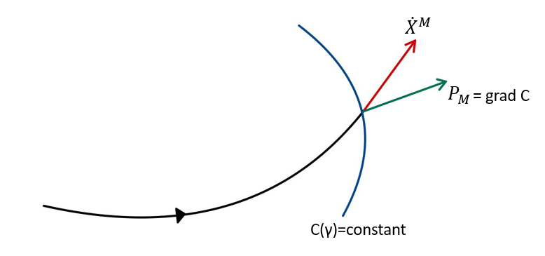
Now, let us consider the principle of minimal complexity from a different perspective, that is, the Hamiltonian mechanics. We first determine the starting and ending points on a configuration space (i.e., $(\gamma(0)=I,t=0)$ and $(\gamma(T)=U,t=T)$), respectively. Next, we assume that the trajectories connecting those points are obtained using Eq. (61), which satisfies Eq. (21). The generalized momentum is defined as

$$P_{M}\equiv\frac{\partial L_{a}}{\partial\dot{X}^{M}},$$

(62)

whose direction is depicited in Fig. 3. Next, we rewrite Eq. (61) as

$$\delta C=\int_{0}^{T}\left\{\frac{\partial L_{a}}{\partial\dot{X}^{M}}\delta\dot{X}^{M}+\frac{\partial L_{a}}{\partial X^{M}}\delta X^{M}\right\}\mathrm{d}t.$$

(63)

By substituting Eq. (21) into this equation and assuming a small variation at the endpoint, namely $\delta\gamma(T)=\delta\gamma\not=0$, Eq. (61) is reformulated as

	$\displaystyle\delta C$	$\displaystyle=\int_{0}^{T}\left\{\frac{\partial L_{a}}{\partial\dot{X}^{M}}\delta\dot{X}^{M}+\frac{\mathrm{d}}{\mathrm{d}t}(\frac{\partial L_{a}}{\partial\dot{X}^{M}})\delta X^{M}\right\}\mathrm{d}t$		(64)
		$\displaystyle=\int_{0}^{T}\frac{d}{dt}\left\{\frac{\partial L_{a}}{\partial\dot{X}^{M}}\delta X^{M}\right\}\mathrm{d}t$
		$\displaystyle=P_{M}\delta X^{M}.$

We take the limit $\delta\gamma\to 0$¹⁵¹⁵15In Lagrangian mechanics, we always assume the variations of endpoints to be zero when deriving the Euler-Lagrange equation. Why do we need to consider an infinitesimal nonzero variation at the endpoint when deriving the HJ equation, though the Euler-Lagrange equation and the HJ equation can be used to describe the same classical system? The difference comes from different essential settings. In Lagrangian mechanics, we identify the equation of motions by varying trajectories between two fixed endpoints. However, when deriving the HJ equation, we consider that the trajectory satisfies the equation of motion. Therefore, instead of varying trajectories, we infinitesimally vary the endpoint of the trajectory to study the corresponding change of the action. So does for the same case in complexity story. In particular, 59 ; 60 have investigated a specific dynamic law, i.e., the first law of complexity by studying the variation of a trajectory’s endpoint in the complexity geometry., such that $P_{M}=\frac{\partial C}{\partial X^{M}}$. Thus, the complexity can be regarded as a functional of $\gamma$, and its infinitesimal variation is written as

$$\delta C=\frac{\partial C}{\partial X^{M}}\delta X^{M}+\frac{\partial C}{\partial t}\mathrm{d}t.$$

(65)

Dividing its both sides by $\mathrm{d}t$ and assuming that $\frac{\mathrm{d}C}{\mathrm{d}t}=L_{a}$ we obtain

$$\frac{\partial C}{\partial t}=L_{a}-P_{M}\dot{X}^{M}=-H_{a},$$

(66)

where $H_{a}$ is the Hamiltonian of the system $\mathcal{A}$ and Eq. (66) represents the HJ equation in the complexity story. However, a new question arises: what is the form of $H_{a}$? We look at the auxiliary Lagrangian, i.e., Eq. (19), in which $P_{M}$ has the following form:

	$\displaystyle P_{M}$	$\displaystyle=\frac{\partial C}{\partial X^{M}}$		(67)
		$\displaystyle=\int_{0}^{T}\frac{\partial L_{a}}{\partial X^{M}}dt$
		$\displaystyle=\int_{0}^{T}\frac{\mathrm{d}}{\mathrm{d}t}\left(\frac{\partial L_{a}}{\partial\dot{X}^{M}}\right)\mathrm{d}t$
		$\displaystyle=G_{MN}\dot{X}^{N}.$

The last equal sign is established because the metric tensor $G_{MN}$ is Hessian 2 , that is, $G_{MN}\equiv\frac{\partial L_{a}}{\partial\dot{X}^{M}\partial\dot{X}^{N}}$. Based on the above construction, we have

$$H_{a}=L_{a}=\frac{1}{2}G_{MN}\dot{X}^{M}\dot{X}^{N},$$

(68)

for which we have

$$\frac{\partial C}{\partial t}+L_{a}=0.$$

(69)

Substituting this into Eq. (57), the computational work is recast as

$$W_{a}(T)=-\int_{0}^{T}L_{a}(t)\mathrm{d}t=-C(T).$$

(70)

We then obtain the equivalent expression of the Jarzynski identity as

$$\mathrm{exp}(-\eta\Delta F_{a}(T))=\left\langle\mathrm{exp}(\eta C(T))\right\rangle.$$

(71)

This equality directly builds a bridge between the computational free energy difference and the complexity.

References

- (1) J. A. Wheeler, Information, Physics, Quantum: The Search for Links, The Proceedings of the 1988 Workshop on Complexity, Entropy, and the Physics of Information, Westview Press, Santa Fe, New Mexico, Boulder, CO, USA (1990).
- (2) J. M. Maldacena, The large-N limit of superconformal field theories and supergravity, Adv. Thoer. Math. Phys. 2, 231 (1998), arXiv:hep-th/9711200.
- (3) S. S. Gubser, I. R. Klebanov and A. M. Polyakov, Gauge theory correlators from noncritical string theory, Phys. Lett. B 428, 105 (1998), arXiv:hep-th/9802109.
- (4) E. Witten, Anti-de Sitter space and holography, Adv. Thoer. Math. Phys. 2, 253 (1998), arXiv:hep-th/9802150.
- (5) S. Ryu and T. Takayanagi, Holographic derivation of entanglement enrtopy from AdS/CFT, Phys. Rev. Lett. 96, 181602 (2006), arXiv:hep-th/0603001.
- (6) L. Susskind, Computational complexity and black hole horizons, Fortschr. Phys. 64, 24 (2016), arXiv:1402.5674.
- (7) D. Stanford, L. Susskind, Complexity and shock wave geometries, Phys. Rev. D 90, 126007 (2014), arXiv:1406.2678.
- (8) L. Susskind, Entanglement is not enough, Fortschr. Phys. 64, 49 (2016), arXiv:1411.0690.
- (9) A. Brown, D. A. Roberts, L. Susskind, B. Swingle and Ying Zhao, Holographic Complexity Equals Bulk Action, Phys. Rev. Lett. 116, 191301 (2016).
- (10) A. Brown, D. A. Roberts, L. Susskind, B. Swingle and Ying Zhao, Complexity, action, and black holes, Phys. Rev. D 93, 086006 (2016), arXiv:1512.04993.
- (11) W. Chemissany, T. Osborne, Holographic fluctuations and the principle of minimal complexity, J. High Energ. Phys. 12, 055 (2016), arXiv:1605.07768.
- (12) M. A. Nielsen, A geometric approach to quantum circuit lower bounds, arXiv:quant-ph/0502070 (2005).
- (13) M. A. Nielsen, M. R. Dowling, M. Gu, and A. C. Doherty, Quantum Computation as Geometry, Scicence 311, 1133 (2006).
- (14) M. A. Nielsen, M. R. Dowling, M. Gu, and A. C. Doherty, Optimal control, geometry, and quantum computing, Phy. Rev. A 73, 062323 (2006), arXiv:quant-ph/0603160.
- (15) M. R. Dowling and M. A. Nielsen, The geometry of quantum computation, arXiv:quant-ph/0701004 (2006).
- (16) A. R. Brown and L. Susskind, The Complexity Geometry of a Single Qubit, Phy. Rev. D 100, 046020 (2019), arXiv:1903.12621.
- (17) R. Auzzi, S. Baiguera, G. B. De Luca, A. Legramandi, G. Naredelli and N. Zenoni, Geometry of quantum complexity, Phy. Rev. D 103, 106021 (2018), arXiv:2001.07601.
- (18) R. Brown and L. Susskind, The Second Law of Quantum Complexity, Phy. Rev. D 97, 086015 (2018), arXiv:1701.01107.
- (19) Wei Sun, Xian-hui Ge, Complexity growth rate, grand potential and partition function, arXiv:1912.00153 (2019).
- (20) Xian-hui Ge, Bin Wang, Quantum computational complexity, Einstein’s equations and accelerated expansion of the Universe, JCAP. 02, 047 (2018), arXiv:1708.06811.
- (21) P. Caputa, J. M. Magan, Quantum Computation as Gravity, Phys. Rev. Lett. 122, 231302 (2019), arXiv:1807.04422.
- (22) C. Jarzynski, Nonequilibrium Equality for Free Energy Difference, Phy. Rev. Lett. 78, 2690 (1997), arXiv:cond-mat/9610209.
- (23) C. Jarzynski, Equilibrium free-energy differences from nonequilibrium measurements: A master-equation approach, Phy. Rev. E 56, 5018 (1997), arXiv:cond-mat/9707325.
- (24) C. Jarzynski, Microscopic analysis of Clausius-Duhem processes, J. Stat. Phys. 96, 415 (1999), arXiv:cond-mat/9802249.
- (25) G. E. Crooks, Nonequilibrium Measurements of Free Energy Differences for Microscopically Reversible Markovian Systems, J. Stat. Phys. 90, 1481 (1998).
- (26) G. E. Crooks, Path-ensemble averages in systems driven far from equilibrium, Phy. Rev. E 61, 2361 (2000), arXiv:cond-mat/9908420.
- (27) G. Hummer, A. Szabo, Free energy reconstruction from nonequilibrium single-molecule pulling experiments, PNAS. 98(7), 3658 (2001).
- (28) C. V. den Brock, M. Esposito, Ensemble and trajectory thermodynamics: A brief introduction, Physica A 418, 6 (2015), arXiv:1403.1777.
- (29) R. P. Feynman, A. R. Hibbs, Quantum Mechanics and Path integrals, Higher Education Press, Beijing (2015).
- (30) M. Kac, On distributions of certain Wiener functionals, Amer. Math. Soc. 65, 1 (1949).
- (31) B. Oeksendal, Stochastic differential equations, Springer, Heidelberg (2000).
- (32) R. P. Feynman, Space-Time Approach to Non-Relativistic Quantum Mechanics, Rev. Mod. Phys. 20, 367 (1948).
- (33) D. Minic, M. Pleimling, The Jarzynski identity and the AdS/CFT Duality, Phys. Lett. B 700, 277 (2011), arXiv:1007.3970.
- (34) N. Y. Halpern, Jarzynski-like equality for the out-of-time-ordered correlator, Phys. Rev. A 95, 012120 (2017), arXiv:1609.00015.
- (35) N. Y. Halpern, A. J. P. Garner, O. C. O. Dahlsten and V. Vedral, Maximum one-shot dissipated work form Rnyi divergences, Phys. Rev. E 97, 052135 (2018).
- (36) S. S. Chern, W. H. Chen and K. S. Lam, Lectures on Differential Geometry, World Scientific, New Jersey (1999).
- (37) J. Maldacena, D. Stanford, Remarks on the Sachdev-Ye-Kitaev model, Phys. Rev. D 94, 106002 (2016).
- (38) J. Maldacena, D. Stanford and Zhenbin Yang, Conformal symmetry and its breaking in two dimensional Nearly Anti-de-Sitter space, PTEP. 2016, 12 (2016), arXiv:1606.01857.
- (39) E. Witten, An SYK-Like Model Without Disorder, J. Phys. A 52, 474002 (2019), arXiv:1610.09758.
- (40) Ying-Fei Gu, Xiao-Liang Qi and D. Stanford, Local criticality, diffusion and chaos in generalized Sachdev-Ye-Kitaev models, J. High Energ. Phys. 2017, 125 (2017), arXiv:1609.07832.
- (41) W. Cottrell, B. Freivogel, D. M. Hofman, S. F. Lokhande, How to Build the Thermofield Double State, J. High Energ. Phys. 02, 058 (2017), arXiv:1811.11528.
- (42) S. Chapman, J. Eisert, L. Hackl, M. P. Heller, R. Jefferson, H. Marrochio and R. C. Myers, Complexity and entanglement for thermofield double states, SciPost Phys. 6, 034 (2017), arXiv:1810.05151.
- (43) C. Spengler, M. Huber, B. C. Hiesmayr, Composite parameterization and Haar measure for all unitary and special unitary groups, J. Math. Phys. 53, 013501 (2012), arXiv:1103.3408.
- (44) A. R. Brown, L. Susskind, Ying Zhao, Quantum Complexity and Negative Curvature, Phys. Rev. D 95, 045010 (2017), arXiv:1608.02612.
- (45) V. I. Arnold, Mathematical Methods of Classical Mechanics, Springer, Heidelberg (1989).
- (46) N. Lashkari, D. Stanford, M. Hastings, T. Osborne and P. Hayden, Towards the fast scrambling conjecture, J. High Energ. Phys. 04, 022 (2012), arXiv:1111.6580.
- (47) Chris G. Gray, Principle of least action, Scholarpedia, 4(12):8291 (2009).
- (48) R. Zwanzig, Nonequilibrium statistical mechanics, Oxford University Press, New York (2000).
- (49) K. Jacobs, Stochastic Processes for Physicists: Understanding Noisy System, Cambridge University Press, Cambridge (2010).
- (50) Z. Schuss, Theory and Applications of Stochastic Processes: An Analytical Approach, Springer, Heidelberg (2010).
- (51) B. E. Baaquie, Path Integrals and Hamiltonians: Principles and Methods, Cambridge University Press, Cambridge (2014).
- (52) D. J. Toms, The Schwinger Action Principle and the Feynman Path Integral for Quantum Mechanics in Curved Space, arXiv:hep-th/0411233 (2004).
- (53) J. H. Van Vleck, The Correspondence Principle in the Statistical Interpretation of Quantum Mechanics, PNAS. 14, 178 (1928).
- (54) C. Morette, On the Definition and Approximation of Feynman’s Path Integrals, Phys. Rev. 81, 848 (1951).
- (55) B. S. DeWitt, Dynamical Theory of Groups and Fields, Gordan and Breach, New York (1964).
- (56) H. S. Ruse, Taylor’s Theorem in the Tensor Calculus, Proc. London Math. Soc. 32, 87 (1931).
- (57) R. Livi, P. Politi, Nonequilibrium Statistical Physics: A Modern Perspective, Cambridge University Press, Cambridge (2017).
- (58) R. P. Feynman, Statistical Mechanics: A Set of Lectures, CRC Press, Los Angeles (2017).
- (59) A. Bernamonti, F. Galli, J. Hernandez, R. C. Myers, Shan-Ming Ruan and J. Sin, First Law of Holographic Complexity, Phys. Rev. Lett. 123, 081601 (2019).
- (60) A. Bernamonti, F. Galli, J. Hernandez, R. C. Myers, Shan-Ming Ruan and J. Sin, Aspects of The First Law of Complexity, arXiv:hep-th/2002.05779 (2020).
- (61) G. Gour, M. P. Müller, V. Narasimhachar, R.W. Spekkens and N. Y. Halpern, The resource theory of informational nonequilibrium in thermodynamics, Phys. Rep. 583, 1 (2015), arXiv:1309.6586.
- (62) F. G. S. L. Brandao, M. Horodecki, J. Oppenheim, J. M. Renes and R. W. Spekkens, Resource Theory of Quantum States out of Thermal Equilibrium, Phys. Rev. Lett. 111, 250404 (2013).
- (63) V. Veitch, S. A. H. Mousavian, D. Gottesman and J. Emerson, The resource theory of stablizer computation, New J. Phys. 16, 013009 (2014).
- (64) E. Chitambar, G. Gour, Quantum resource theories, Rev. Mod. Phys. 91, 025001 (2019).
- (65) M. Horodecki, P. Horodecki and J. Oppenheim, Reversible transformations from pure to mixed states and the unique measure of information, Phys. Rev. A 67, 062104 (2003).
- (66) M. Horodecki, K. Horodecki, P. Horodecki, R. Horodecki, J. Oppenheim, A. Sen(De) and U. Sen, Local Information as a Resource in Distributed Quantum Systems, Phys. Rev. Lett. 90, 100402 (2003).
- (67) L. Susskind, Three Lectures on Complexity and Black Holes, arXiv:1810.11563 (2018).
- (68) N. Y. Halpern, N. B. T. Kothakonda, J. Haferkamp, A. Munson, J. Eisert and P. Faist, Resource theory of quantum uncomplexity, arXiv:2110.11371 (2021).
- (69) L. Susskind and Y. Zhao, Switchbacks and The Bridge to Nowhere, arXiv:1408.2823 (2014).
- (70) S. Vinjanampathy and J. Anders, Quantum Thermodynamics, Contemporary Phys. DOI: 10.1080/00107514.2016.1201896 (2016) arXiv: 1508.06099.
- (71) C. Jarzynski, Equalities and Inequalities: Irreversibility and the Second Law of Thermodynamics at the Nanoscale, Annu. Rev. Condens. Matter Phys. 2, 329 (2011).
- (72) H. B. Callen, T. A. Welton, Irreversibility and Generalized Noise, Phys. Rev. 83, 34 (1951).
- (73) J. Hermans, Simple Analysis of Noise and Hysteresis in (Slow-Growth) Free Energy Simulations, J. Phys. Chem. 95, 9029 (1991).
- (74) G. Camilo, Complexity and Floquet dynamics: Non-equilibrium Ising phase transition, Phys. Rev. B 102, 174304 (2020), arXiv:2009.00069.
- (75) E. Lieb, T. Schultz, D. Mattis, Two soluble models of an antiferromagnetic chain, Ann. Phys. 16, 407 (1961).
- (76) E. Barouch, B. M. McCoy, M. Dresden, Statistical Mechanics of the XY Model. I, Phys. Rev. A 2, 1075 (1970).
- (77) M. S. Kalyan, G. A. Prasad, V. S. S. Sastry, K. P. N. Murthy, A Note on Non-equilibrium Work Fluctuations and Equilibrium Free Energies, J. Phys. A 390, 1240 (2011), arXiv:1011.4413.
- (78) M. Esposito and C. V. den Broeck, Three detailed fluctuation theorems, Phys. Rev. Lett. 104, 090601 (2010).
- (79) R. Jefferson, R. C. Myers, Circuit complexity in quantum field theory, J. High Energ. Phys. 2017, 107 (2017), arXiv:1707.08570.
- (80) R. Jefferson, R. C. Myers, Circuit complexity in quantum field theory, J. High Energ. Phys. 2017, 107 (2017), arXiv:1707.08570.
- (81) Run-Qiu Yang, Yu-Sen An, Chao Niu, Cheng-Yong Zhang, Keun-Young Kim, What kind of "complexity" is dual to holographic complexity, arXiv:2011.14636 (2021).
- (82) L. Bassman, K. Klymko, N. M. Tubman and Wibe A. de Jong, Computing Free Energies with Fluctuation Relations on Quantum Computers, arXiv:2103.09846 (2021).
- (83) K. Jacobs, Stochastic Processes for Physicits: Understanding Noisy Systems, Cambridge University Press, Cambridge (2010).
- (84) G. S. Chirikjian, Stochastic Models, Information theory, and Lie Groups, Springer, Heidelberg (2000).
- (85) J. Schwinger, The Theory of Quantized Fields. I, Phys. Rev. 82, 914 (1951).
- (86) J. Schwinger, The Theory of Quantized Fields. II, Phys. Rev. 91, 713 (1953).
- (87) Qiuping A. Wang, Maximum path information and the principle of least action for chaotic system, Chaos, Solitons & Fractals 23, 1253 (2005), arXiv:cond-mat/0405373.
- (88) https://brilliant.org/wiki/markov-chains/markov-chain.