Toward Performance-Portable PETSc for GPU-based Exascale Systems
Abstract
The Portable Extensible Toolkit for Scientific computation (PETSc) library delivers scalable solvers for nonlinear time-dependent differential and algebraic equations and for numerical optimization. The PETSc design for performance portability addresses fundamental GPU accelerator challenges and stresses flexibility and extensibility by separating the programming model used by the application from that used by the library, and it enables application developers to use their preferred programming model, such as Kokkos, RAJA, SYCL, HIP, CUDA, or OpenCL, on upcoming exascale systems. A blueprint for using GPUs from PETSc-based codes is provided, and case studies emphasize the flexibility and high performance achieved on current GPU-based systems.
keywords:
numerical software , high-performance computing , GPU acceleration , many-core , performance portability , exascaleMSC:
[2010] 65F10 , 65F50 , 68N99 , 68W101 Introduction
High-performance computing (HPC) node architectures are increasingly reliant on high degrees of fine-grained parallelism, driven primarily by power management considerations. Some new designs place this parallelism in CPUs having many cores and hardware threads and wide SIMD registers: a prominent example is the Fugaku machine installed at RIKEN in Japan. Most supercomputing centers, however, are relying on GPU-based systems to provide the needed parallelism, and the next generation of open-science supercomputers to be fielded in the United States will rely on GPUs from AMD, NVIDIA, or Intel. These devices are extremely powerful but have posed fundamental challenges for developers and users of scientific computing libraries.
This paper shows how to use GPUs from applications written using the Portable, Extensible Toolkit for Scientific computation (PETSc, [1]), describes the major challenges software libraries face, and shows how PETSc overcomes them. The PETSc design completely separates the programming model used by the application and the model used by PETSc for its back-end computational kernels; see Figure 1. This separation allows PETSc users from C/C++, Fortran, or Python to employ their preferred GPU programming model, such as Kokkos, RAJA, SYCL, HIP, CUDA, or OpenCL [2, 3, 4, 5, 6, 7], on upcoming exascale systems. In all cases, users will be able to rely on PETSc’s large assortment of composable, hierarchical, and nested solvers [8], as well as advanced time-stepping and adjoint capabilities and numerical optimization methods running on the GPU.
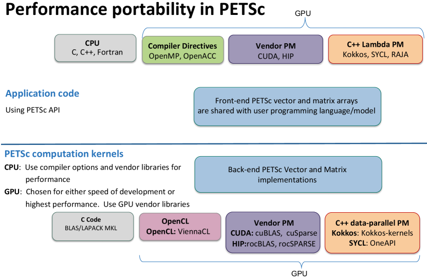
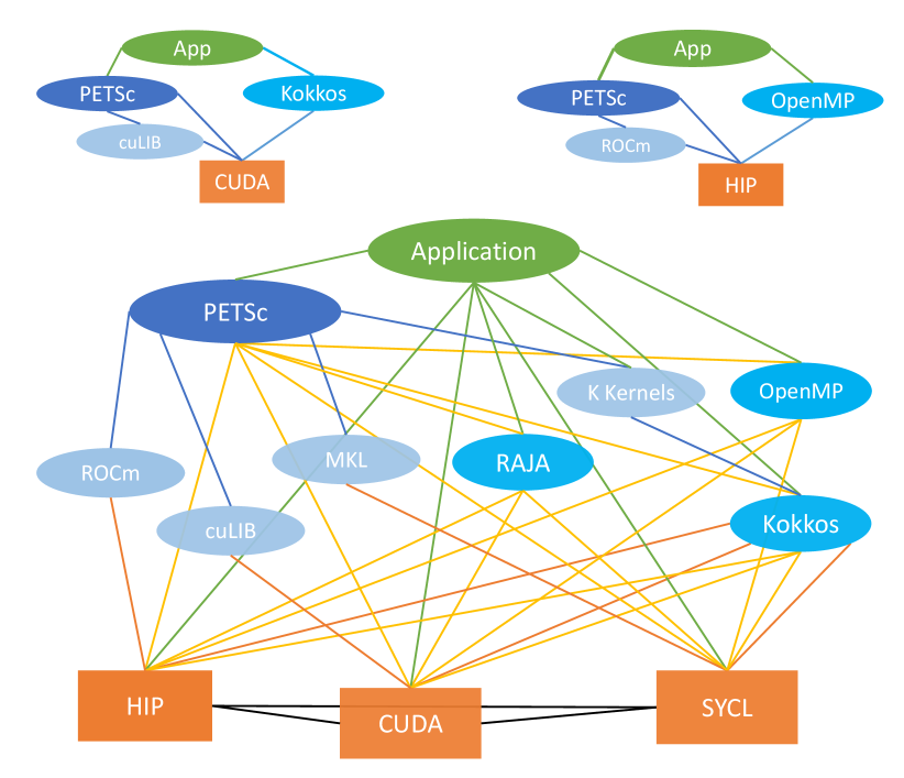
An application for solving time-dependent partial differential equations, for example, may compute the Jacobian using Kokkos and then call PETSc’s time-stepping routines and algebraic solvers that use CUDA, cuBLAS, and cuSPARSE; see Figure 2. Applications will be able to mix and match programming models, allowing, for example, some application code in Kokkos and some in CUDA. The flexible PETSc back-end support is accomplished by sharing data between the application and PETSc programming models but not sharing the programming models’ internal data structures. Because the data is shared, there are no copies between the programming models and no loss of efficiency.
GPU vendors and the HPC community have developed various programming models for using GPUs. The oldest programming model is CUDA, developed by NVIDIA for their GPUs. AMD adopted an essentially identical model for their hardware, calling their implementation HIP. Several generations of the OpenCL programming model, supported in some form by NVIDIA, AMD, and Intel, have been designed for portability across multiple GPU vendors’ hardware. Moreover, there are the C++ data-parallel programming models that make use of C++ lambdas and provide constructs such as parallel_for for programmers to easily express data parallelism that can be mapped by the compilers into GPU-specific implementations. To some degree, they are C++ variants of the CUDA model. The oldest is Kokkos [2], which has support for CUDA, HIP, DPC++, and shared-memory OpenMP, but not for OpenCL. RAJA [3] was introduced more recently. SYCL [4] is a newer model that typically uses OpenCL as a back-end. A notable SYCL implementation is DPC++ [9], developed by Intel for its new discrete GPUs. Figure 2 (upper right) shows the case where the application uses OpenMP offload and runs on a HIP system and (bottom) the entire web of potential programming models and back-end numerical libraries that will be employed by PETSc.
This paper is organized as follows. We first provide a blueprint for porting PETSc applications to use GPUs. We next survey the challenges in developing efficient and portable mathematical libraries for GPU systems. We then introduce the PETSc GPU programming model and discuss recent PETSc back-end developments designed to meet these challenges. We present a series of case studies using PETSc with GPUs to demonstrate both the flexible design and the high performance achieved on current GPU-based systems. In the final section we summarize our conclusions. Throughout this paper, we use the term “programming model” to refer to both the model and its supporting runtime.
2 Porting PETSc applications to the GPUs
The common usage pattern for PETSc application codes, regardless of whether they use time integrators, nonlinear solvers, or linear solvers, has always been the following:
-
•
Setup application data, meshes, initial state, etc.,
-
•
provide a callback for the Function that defines the problem (e.g., nonlinear residual, ODE right-hand side),
-
•
provide a callback for the Jacobian of the Function
-
•
call the PETSc solver, possibly in a loop.
This approach does not change with the use of GPUs. In particular, the creation of solver, matrix, and vector objects and their manipulation do not change. Points to consider when porting an application to GPUs are:
-
•
Some data structures reside in GPU memory, either
-
•
constructed on the CPU and copied to the GPU or
-
•
constructed directly on the GPU.
-
•
-
•
Function will call GPU kernels.
-
•
Jacobian will call GPU kernels.
The recommended approach to port PETSc CPU applications to the GPU is to incrementally move the computation to the GPU:
-
•
Step 1: write code to copy the needed portions of already computed application data structures to the GPU.
-
•
Step 2: write code for Function that runs partially or entirely on the GPU.
-
•
Step 3: write code for Jacobian that runs partially or entirely on the GPU.
-
•
Step 4: evaluate the time that remains from building the initial application data structures on the CPU.
-
•
If the time is inconsequential relative to the entire simulation run, the port is complete;
-
•
otherwise port the computation of the data structure to the GPU.
-
•
When developing code, the developer should add the new code to the existing code and use small stub routines (see Listing 4) that call the new and the old functions and compare the results as the solver runs, in order to detect any discrepancies. We further recommend postponing additional refactorizations until after the code has been fully ported to the GPU, with testing, verification, and performance profiling performed at each step of the transition. For convenience, in the rest of this section we focus on an application using Kokkos; a similar process would be followed for SYCL, RAJA, OpenMP offload, CUDA, and HIP. We recommend using the sequential non-GPU build of Kokkos for all development; this allows debugging with traditional debuggers.
Listing 1 displays an excerpt of a typical PETSc main application program for solving a nonlinear set of equations on a structured grid using Newton’s method. It creates a solver object SNES, a data management object DM, a vector of degrees of freedom Vec, and a Mat to hold the Jacobian. Then, Function and Jacobian evaluation callbacks are passed to the SNES object to solve the nonlinear equations.
Listing 2 shows a traditional PETSc (top) and a Kokkos implementation (bottom) of Function. DMDAVecGetArrayRead sets the correct dimensions of the array that lies on each MPI rank. XxxRead/Write here claims the caller will only read or write the returned data. These functions are similar in the Kokkos version except that they do not require the Read/Write labels for the accessor routines (these are handled by using the appropriate const qualifiers in the overloaded functions, not shown). When returning OffsetViews, we wrap but do not copy PETSc vectors’ data. Moreover, in the Kokkos version we use the parallel_for construct and determine the loop bounds from the OffsetView. For simplicity of presentation we have assumed periodic boundary conditions in one dimension; the same code pattern exists in two and three dimensions with general boundary conditions. When porting code with nontrivial boundary conditions, one should first port the main loop, test and verify that the code is still running correctly, and then incrementally port each boundary condition separately, testing for each.
The Jacobian computation is presented in Listing 3. The callbacks are also similar except for the matrix access request in the Kokkos version.
In Listing 4, we conclude with the crucial stub function. This stub has the same calling sequence as the two functions that are to be compared and can be passed directly to the solver routine to verify that both produce the same results while solving the equations.
3 Challenges in GPU programming for libraries
Three fundamental challenges arise in providing libraries that obtain high throughput performance on parallel GPU accelerated systems because of the hardware and low-level software aspects of the GPUs; no programming model obviates or allows programmers to ignore them. These fundamental challenges are labeled with an F. Ancillary challenges arise in the process of meeting the fundamental challenges; these are labeled with an A.
Challenge F1: Portability for application codes
The first challenge for GPUs’ general use in scientific computing is the portability of application code across different hardware and software stacks. Different vendors support different programming models and provide different mathematical libraries (with different APIs) and even different synchronization models. AMD is revising its HIP and ROCm library support; how closely it will mimic the CUDA (cuBLAS, cuSPARSE) standards is unclear. On the other hand, NVIDIA continues to develop the cuSPARSE API, deprecating and refactoring many common usage patterns for sparse matrix computations. Kokkos is designed to guarantee application codes’ portability, but it does not provide distributed-memory MPI support and requires the user to work in its particular C++ programming style. Likewise, OpenCL has portable performance as an overarching goal, but implementation quality has been uneven, and performance has not met the standard needed for many application codes [10]. OpenMP offload poses unique difficulties for libraries. Since it is compiler based and the data structures and routines are opaque, it may require specific code for each OpenMP implementation.
Challenge F2: Algorithms for high-throughput systems
In addition to application porting, high-throughput systems such as GPUs require developing and implementing new solver algorithms—in particular, algorithms that exploit high levels of data-parallel concurrency with low levels of memory bandwidth delivered in a data-parallel fashion. This approach generally involves algorithms with higher arithmetic intensity than most traditional simulations require. This challenge is beyond the scope of this paper; a robust research program developing advanced algorithms for GPU-based systems is being undertaken by the PETSc team and their collaborators.
Challenge F3: Utilizing all GPU and CPU compute power
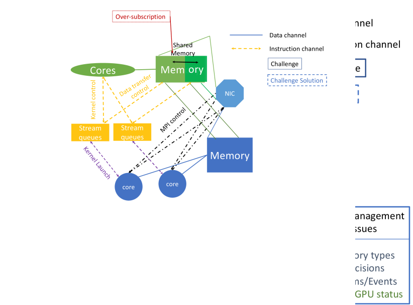
The current focus of the PETSc library work for GPUs is high computational throughput for large simulations, keeping all the GPU compute units as busy as possible all of the time. In order to achieve this, each core must have an uninterrupted stream of instructions and a high-bandwidth stream of data within the constraints of the hardware and low-level software stack. The difficulty arises from the complex control flows and data flows, as indicated in Figure 3. With distributed-memory GPU computing, two levels of instruction flow exist:
-
•
high-level instructions flow from the CPU memory to the GPU stream queue and the GPU memory controller, and
-
•
kernel code flows from the GPU memory to the GPU compute cores.
The two levels of data flow are
-
•
between GPU memories through a combination of networks, switches, and RDMA transfers and
-
•
between the GPU memory and the GPU compute cores.
In this work, we are concerned only with the high-level instruction and data flow and assume that the low-level is suitably handled within the computational kernels and the hardware.
With a high-throughput computation on the GPU and the CPU cores, the same basic rule applies. Seamless high-level data control must exist between the CPU memory and the GPU memory, and the high-level instruction flow for the CPUs and GPUs must be coordinated and synchronized to ensure that neither is interrupted.111The OLCF Summit IBM/NVIDIA system includes an additional layer, whereby data control for transfers directly from the CPU caches to the GPU memory, but this will be ignored. Since the exascale nodes have many more CPU cores than GPUs, a mismatch exists between the two for both high-level instruction management and data flows; this is called the oversubscription problem.
For both the pure GPU throughput problem and the combined CPU and GPU case, one must understand in a little more detail how the CPU controls the GPU operation. The CPU sends two types of high-level instructions to the stream queue on the GPU:
-
•
Kernel launch instructions that control the next set of low-level instructions the GPU will run on its compute cores
-
•
Data transfer instructions that control the movement of data
High-level instructions are issued in the order they arrive in the queue. Should the queue become empty, the GPU computations and memory transfers will cease. One of the most challenging problems currently faced by large-scale distributed-memory GPU-based computing is preventing this queue from becoming empty. It is crucial that more entries be added to the queue without requiring the queue to be emptied first. The process of adding more entries while the queue is not empty is called pipelining.
Challenge A1: Managing the kernel queue
Two other techniques besides pipelining can keep the GPU compute cores busy.
One approach is kernel fusion, which combines multiple kernels into a single kernel to increase the time spent in kernel computations while reducing the number of kernel launches, with the additional benefit of possibly increasing the arithmetic intensity of the computations. However, this optimization often results in code that is harder to read and more difficult to maintain. For thirty years, the general model for library development has been to write short single-concern functions that can be easily combined to promote code reuse. PETSc uses this style where each concern is its class method.
A second approach is using CUDA graphs, which allow the user to describe a series of operations (including CUDA kernels) and their dependencies as a graph. These graphs can be instantiated once and then executed many times without involving the CPU to amortize the high instantiation cost. This approach is similar to pipelining except that it offers more runtime flexibility in determining the next operation within the GPU based on the state of the computation, whereas with pipelining the order of operations is set in advance by the CPU.
Challenge A2: Network communication
GPU-aware MPI was introduced to hide latency and ease development of multi-node GPU code by allowing MPI calls to accept GPU memory address pointers, thereby allowing MPI implementations to overlap GPU-CPU copies with communication rendezvous, chunking, and completion, as well as on-node optimizations. For example, a CUDA-aware MPI can use NVIDIA GPUDirect point-to-point to copy data between two GPUs within a compute node or use NVIDIA GPUDirect RDMA to access the remote GPU memory across compute nodes without requiring CPU involvement.
Unfortunately, at the time of writing, even GPU-aware MPI implementations cannot pipeline MPI calls and kernel launches because the MPI API does not utilize the stream queue. Figure 3 shows that the GPU-aware MPI instructions pass directly to the memory controls (the black dashed lines) and do not enter the stream queue. Thus, the stream queue must be empty for every MPI call. Such expensive GPU synchronization for every MPI call involving GPU memory embodies the mismatch between MPI and GPU. This problem is analyzed in more detail in [11].
In contrast, NVIDIA provides both NCCL [12], a library of multi-GPU collective communication primitives, and NVSHMEM [13], an implementation of the OpenSHMEM [14] communications model for clusters of NVIDIA GPUs. Unlike MPI, these libraries can initiate communication from the CPU on streams to synchronize between computation and communication taking place on the GPU. NVSHMEM also supports GPU-initiated communication.
Challenge A3: Over- and undersubscription
Exascale systems will have many more CPU cores than GPUs, and applications may use both the CPU and the GPU for their computations. Libraries and applications must manage the mismatch between the number of cores and GPUs. Two main alternatives can help manage this challenge.
Oversubscription occurs when multiple CPU processes use the same GPU simultaneously. On high-end NVIDIA systems, the Multi-Process Service (MPS), a runtime system enabling multiprocess CUDA applications to transparently use the Hyper-Q hardware-managed work queues on the GPU, allows funneling the work from multiple CUDA contexts into a single context. In some cases, this can improve resources utilization, but it can also reduce GPU efficiency. On Summit, for instance, we have observed reductions between 5% and 20% when sharing GPUs between ranks. Many types of overhead can contribute to this reduced efficiency, but we group them all as GPU oversubscription overhead. For example, in a standard strong scaling regime, increasing the number of processes sharing the same GPU while holding the computational load per physical GPU constant may result in more kernel launches associated with smaller chunks of data, ultimately degrading performance. It is unclear what this overhead will be on future systems.
A variant of this approach maintains two communicators, one for all the MPI processes and one with a single process for each physical GPU. While the GPUs can be used at all times, control of the GPUs may be dropped down to the smaller communicator during intense phases of GPU utilization. The individual ranks’ data in the GPU memory can be shared with the GPU’s single-rank process via interprocess communication (e.g., cudaIpc) calls. Alternatively, all the extra CPU cores associated with the GPU controlling rank can share a small communicator over which the needed communication is performed, either by using MPI shared-memory windows or via scatter/gather operations.
A different approach is to always use one MPI rank per GPU and use, for example, OpenMP shared-memory programming to employ additional cores controlled by the single MPI rank that also controls the GPU. When individual library or application components use pure MPI and others use hybrid MPI-OpenMP, a decrease in active ranks is also necessary.
Undersubscription occurs when a large computation has short phases that are best computed on a smaller set of the computational cores, in other words, fewer GPUs and CPUs; this is commonly encountered in coarse level solves of a multigrid algorithm. A complete library system must manage the reduction in computational cores used and the efficient movement of data required to utilize the fewer resources and the transition back to the full system.
Challenge A4: CPU-GPU communication time
CPU-GPU communications can limit the application’s overall performance. The best approach to deal with the communication costs is to reduce the amount of communication needed by moving computation to the GPU. Communication can also overlap with computation on the GPU by performing the computations in different streams.
On NVIDIA and AMD GPUs, the communication time can be reduced by using pinned memory. Pinned memory is CPU memory whose pages are locked to allow the RDMA system to employ the full bandwidth of the CPU-GPU interconnect; we observed bandwidth gains up to a factor of 4.
Challenge A5: Multiple memory types
When running on mixed CPU and NVIDIA GPU systems, there are at least four types of memory: regular memory on the CPU, pinned memory, unified shared memory, and GPU memory. The first is usable only on the CPU; the second may be usable on some GPUs, but not directly via the host pointer; the third is usable on both the CPU and GPU; and the fourth only on the GPU. Pointers for all of them are allocated, managed, and freed by the CPU process. AMD’s HIP API and Intel’s discrete GPUs add to the diversity of memory models that library and application developers must support to achieve optimal performance across all systems.
When multiple types of memory are used, especially by different libraries, there must be a system to ensure that the appropriate version of a function is called for the given memory type. CUDA provides routines to determine whether the memory is GPU or CPU, but these calls are expensive (about 0.3 s on OLCF Summit) and should be avoided when possible. OpenMPI and MPICH implementations that are GPU-aware call these routines repeatedly and thus pay this latency cost for each MPI call involving memory pointers. With unified memory, the operating system automatically manages transferring pages of unified memory between the CPU and GPU. However, this approach means that callers of libraries using unified memory must ensure they use the correct memory type in application code; otherwise, expensive data migration will be performed in the background.
Challenge A6: Use of multiple streams from libraries
Multiple streams are currently used by NVIDIA and AMD systems to synchronize different computation and computation phases directly on the GPU by providing multiple stream queues. This synchronization is much faster than synchronizations done on the CPU. Care must be taken not to launch too many overlapping streams, however, since they can slow the rate of the computation. Thus, it is best that a single entity be aware of all the streams; this requires extra effort when different libraries are all using streams. Moreover, if different libraries produce computations that require synchronizations between the library calls, those libraries must share common streams.
Challenge A7: Multiprecision on the GPU
GPU systems often come with more single-precision than double-precision floating-point units. Even bandwidth-limited computations with single precision can be faster because they require half of the double-precision computations’ memory bandwidth. Sparse matrix operations do not usually see dramatic improvements, however, because the integer indices remain the same size.
With the compressed sparse row matrix format, the amount of data that needs to be transferred from the matrix is for double-precision computations with 32-bit column indices and for single-precision computations, a ratio. Further reductions in the factor require compression of the column indices or using a different storage format; see, for example, [15].
Recent GPUs also contain tensor computing units that use 16-bit floating-point operations. These are specialized and do not provide general-purpose 16-bit floating-point computations, but they have significant computing power; they can be used effectively for dense [16] or even sparse matrix computations [17]. See also a recent survey on multiprecision computations for GPUs [18].
4 Progress on PETSc’s back-end for GPUs
PETSc employs an object-oriented approach with the delegation pattern; every object is an instance of a class whose data structure and functionality is provided by specifying a delegated implementation type at runtime. For example, a matrix in compressed sparse row representation is created as an instance of class Mat with type MATAIJ, whereas a sliced ELLPACK storage matrix has type MATSELL. We refer to the API of the classes that the user code interacts with front-end while we call the delegated classes the back-end. Using GPUs to execute the linear algebra operations defined over Vec and Mat is accomplished by choosing the appropriate delegated class. For instance, the computations will use the vendor-provided kernels from NVIDIA if VECCUDA and MATAIJCUSPARSE are specified in user code or through command line options. Because the higher-level classes such as the timesteppers TS ultimately employ Vec and Mat operations for the bulk of their computations, this provides a means to offload most of the computation for PETSc solvers—even the most complicated and sophisticated—onto GPUs.
The GPU-specific delegated classes follow the lazy-mirror model [19]. These implementations internally manage (potentially) two copies of the data—one on the CPU and one on the GPU—and track which copy is current. When the computation for that data is always on the GPU, there is no copy back to the CPU. When a GPU implementation of a requested operation is available, the GPU copy of the data is updated (if needed), and the GPU-optimized back-end class method is executed. Otherwise, the CPU copy of the data is updated (if needed), and the CPU implementation is used. (Further details of this approach are given in Response A4 of this section.)
This mechanism offers two advantages [20]. First, the full set of operations for the Vec and Mat classes is always available, and developers can incrementally add more back-end class methods as execution bottlenecks become apparent. Second, some operations are difficult or impossible to implement efficiently on GPUs, and using the CPU implementation offers acceptable or even optimal performance.
When unified shared memory is available, the PETSc back-end classes could allocate only a single unified buffer for both the CPU and GPU and allow the operating system to manage the CPU and GPU movement. However, having PETSc manage the memory transfers itself may result in better performance.
Response F1: Portability for application codes
Each PETSc back-end comprises two parts: the calls to numerical libraries that provide the per GPU algorithmic implementation and the glue code that connects these calls to the front-end code. The numerical libraries are cuBLAS and cuSPARSE for the CUDA back-end, ROCm for HIP, ViennaCL [21] for OpenCL (and potentially also for CUDA and HIP), MKL for SYCL, and Kokkos Kernels for Kokkos. Different PETSc back-end subclasses can be used in the same application.
Our highest priority at present is to prepare for the upcoming exascale systems. We already have a working Kokkos Kernels back-end. We are completing the HIP back-end to exploit the AMD GPUs planned for the upcoming Frontier system at Oak Ridge National Laboratory. The basic configuration for HIP is in place, as well as the initial vector operations. Development is in progress and being tested on early-access testbeds for Frontier. We have also begun implementation for a SYCL and MKL back-end for use with the Intel GPUs planned for the Aurora system at Argonne National Laboratory.
As our computation kernels’ development continues, we are also abstracting the fundamental types, their initialization, and the various libraries’ interfaces to reduce code duplication. The PETSc team will work with the Intel and AMD compiler groups to determine the information needed from the OpenMP offload compiler to share its data with the PETSc back-end.
Response F3: Utilizing all GPU (and CPU) compute power
Achieving high utilization requires a rethinking of outer-level algorithms to take advantage of operations with higher arithmetic intensity. Compact, dense quasi-Newton representations present an avenue for increasing arithmetic intensity and increasing GPU utilization for outer-level algorithms. Compared with conventional limited-memory matrix-free implementations, these formulations require fewer kernel launches, avoid dot products, and compute the approximate Jacobian action via a sequence of matrix-vector products constructed from accumulated quasi-Newton updates. Initial support for solving Krylov methods with multiple right-hand sides has been added to PETSc [22]. While having higher arithmetic intensity, these methods generate larger Krylov subspaces and typically converge in fewer iterations, and they may thus provide algorithmic speedup for calculating eigenvalues and for multiobjective adjoint computations. These block methods significantly decrease the number of sequentially launched kernels, providing outer loop fusion that reduces CPU-GPU latencies and calls; see challenge F2. Even with the multiple right-hand side optimizations, NVIDIA’s cuSPARSE on a V100 with extremely sparse matrix-vector multiplication achieves only 4% of peak, thus indicating the desirability of implementing algorithms that fundamentally change the performance for such simulations. Outer loop fusion will also be applied for other PETSc operations such as the multiple dot products operations needed in the Krylov methods (replacing a collection of BLAS 1 operations with a single BLAS 2 operation) to reduce the number of kernel launches and get more data reuse on the GPU and higher utilization.
A cross-utilization of the CPU and GPUs can occur even within what is conceptually a single computation. Consider the computation of matrix elements for a discretization scheme and their insertion into a matrix data structure. Within PETSc, value insertion is performed in a loop with the general routine MatSetValues (usage depicted in Listing 3), which efficiently adjusts the row sizes on the fly as values are inserted and takes care of communicating off-processor values, if needed.
However, the many repeated calls to MatSetValues run on the CPU and may cause a bottleneck when the assembling process runs on a GPU. To address this issue, we have developed a variant of the function callable from kernels that will guarantee fast GPU resident assembly. In a somewhat different scenario, common among complicated applications utilizing PETSc only for its robust solver functionality, the matrix values can be already available from the application itself; for such cases, we have recently developed a new API that accepts a general matrix description in a coordinate list (COO) format and directly assembles on the GPU utilizing efficient kernels from the Thrust library that is part of the CUDA Toolkit. For numerical results, see Section 5.5.
PETSc will use the simultaneous kernel launch capability of NVSHMEM to begin its parallel solvers, thus making them more tightly integrated and remaining in step during the solve process. This is a relatively straightforward generalization of the current solver launches, and it will be opaque to the users.
The PETSc back-end model is designed to support applications and libraries using a combination of CPUs and GPUs for computations. Each back-end class implementation provides two implementations, for host and device, and contains the code to manage data transfers. This strategy allows the users of PETSc to prescribe the next group of computations to take place by merely setting a flag on the object. With this approach, running, for example, the coarser levels of multigrid on the CPU and the finer levels on the GPU is easy. Unnecessary GPU-to-CPU communication is avoided with this approach, and any needed communication is handled internally by the object. The associated message passing required by the solver is managed automatically by PetscSF; see Response A2.
Response A1: Managing the kernel queue
Since MPI does not use streams, inner products and ghost point updates require a CPU synchronization at these steps; one cannot, for example, pipeline an entire iteration of a solver together. We will provide support for NVSHMEM to allow the communication to utilize the stream queue; see Response A2. This is an important addition to PETSc to eliminate the empty streams queue problem.
Response A2: Network communication
PetscSF is the PETSc communication module, which has a simple but powerful interface to simplify communication code on both CPUs and GPUs [23]. It manages proper synchronizations needed by GPU-aware MPI, and has a series of optimizations to improve communication performance. PetscSF is incrementally replacing all direct use of MPI in PETSc. This will allow PETSc to utilize the features of NVSHMEM that are required to eliminate the problems of Challenge A2.
PetscSF uses the abstraction of star forests to represent communication patterns. A star is a simple tree consisting of one root vertex connected to zero or more leaves. A star forest is a disjoint union of stars. A PetscSF is created collectively by specifying, for each leaf on the current rank, the rank and offset of the corresponding root, shown in Figure 4. PetscSF then analyzes the graph and derives a communication pattern using persistent nonblocking MPI send and receive (default), other collectives, one-sided, or neighborhood collectives. PetscSF provides APIs such as PetscSF{Bcast,Reduce}Begin/End. The former broadcasts root values to leaves, and the latter reduces leaf values into roots with an MPI_Op. The Begin/End split-phase design allows users to insert computations in between, in order to overlap with communication.
Root and leaf indices are typically not contiguous per rank, so that the library has to pack and unpack the data for MPI sends and receives. If the data is in GPU memory, these pack/unpack routines must be implemented in GPU kernels. PetscSF APIs are raw pointer-based, for example,
where unit defines the data type of the vertices in the graph. PetscSF originally used cudaPointerGetAttributes to infer root/leaf memory spaces, but that turned out to slow down the operations, so we now keep track of the memory types that are passed to the PetscSF for communication on PETSc vectors. Currently, PetscSF supports CUDA and Kokkos; support for HIP and SYCL will be added soon. We will also provide a back-end that uses NVSHMEM or NCCL.
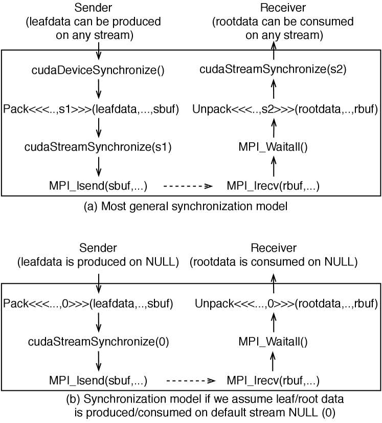
PetscSF prefers GPU-aware MPI, but it also supports non-GPU-aware MPI. Here we discuss some of the details of our GPU-aware support. There are multiple choices to build synchronization models, as shown in Figure 5, which uses CUDA as an example. In Figure 5(a), we assume that leafdata is produced by a kernel on a stream unknown to PetscSF. Therefore the sender has to call CUDADeviceSynchronize to synchronize with all the computations on the GPU before the pack kernel in order to make sure the leafdata is ready to pack. After the pack, the implementation calls CUDAStreamSynchronize(s1) to synchronize stream s1 and make sure the packed data in sbuf is ready for MPI_Isend. On the receiver side, when the MPI_Waitall returns, the received data is guaranteed to be in the receive buffer rbuf. But we might have to call the unpack kernel, for example, on stream s2, to unpack the data from rbuf to rootdata and call CUDAStreamSynchronize(s2) to synchronize unpack so that rootdata can be consumed by kernels on any stream.
Manipulating multiple streams
is not an easy task. Like most codes, the PETSc default is to use only the
default stream. A simplified synchronization model is shown in Figure
5(b), where we launch pack/unpack on
the default stream and omit the CUDADeviceSynchronize before
pack and CUDAStream
Synchronize(s2) after unpack. But
obviously, we still need
CUDAStreamSynchronize(NULL)
before MPI_Isend.
A solution for the MPI-GPU mismatch problem is to expose the CUDA streams to the MPI API; doing so will allow MPI function calls on GPU memory
to behave more like kernels where the user selects the appropriate streams to allow
kernel pipelining.
The MPI Forum has begun an Accelerator working group, and the PETSc team is an eager
customer willing to quickly work with the prototypes the working group develops.
MPI processes often need to communicate with themselves as well. Traditionally, programmers chose not to distinguish local (i.e., self-to-self) and remote (i.e., self-to-others) communications and let MPI handle the distinction, resulting in a simpler and more uniform user code. Distinguishing these types of communications with GPU computation is essential, however. At least two benefits accrue: (1) we can directly scatter source data to its destination without intermediate send or receive buffers for local communication, and (2) local communication is done by a GPU kernel (doing a memory copy with index indirection). The kernel can be perfectly executed asynchronously with remote MPI communication, overlapping local and remote communications.
PetscSF performs index analysis at the setup phase to provide optimizations to lower the cost on GPUs further. If leaf or root indices are contiguous, we do not need pack/unpack and intermediate buffers: data can be sent directly to save kernel launch and execution time. For noncontiguous indices, the indices might have specific patterns that can be taken advantage of to reduce the packing or unpacking time. Currently, PetscSF can detect whether a set of indices are for points in a rectangular subdomain. For example, in a rectangular 3D domain, the ghost regions (faces) and interior region are all such qualified subdomains. Packing entries in such subdomains only need parameters describing the subdomains, instead of all entry indices. Also, in PetscSFReduce, multiple leaves might be reduced into the same root. If so, the unpack kernel needs to take care of the data race between threads. Instead of blindly using atomic operations all the time, PetscSF leverages index analysis, and it uses nonatomic instructions when no duplicated indices are found.
Response A3: Oversubscription
We are focusing on the most critical case for PETSc exascale application codes: simulations that perform phases of the computations jointly on the CPUs and GPUs, with other phases exclusively on the GPUs all using a purely MPI model. This case will use the approach outlined above, using a large MPI communicator for all MPI cores with shared process usage of the GPUs combined with a smaller communicator just for the GPUs with the highest performance single process usage of the GPUs. Since the bulk of the computation will take place without sharing the GPU, this approach tolerates the overhead that arises from sharing mentioned in Challenge A3. Shared memory on the GPUs will allow joint ownership of the data used in the different phases of the computation; communication for the data will be managed by PetscSF, transparent to the application code. Other use cases can easily be added as needed by the application teams. PetscSF will also provide transparent support for the undersubscription problem faced, for example, by multigrid; see Section 5.3.
Response A4: GPU-CPU communication time
PETSc, by default, uses pinned memory for all data that may be copied to or from the GPU memory. As mentioned above, PETSc uses the lazy-mirror model to reduce memory copies. At the lowest level of the PETSc software stack, data access is controlled via get operations such as VecGetArrayRead, VecGetArrayWrite, and VecGetArray, and the corresponding restoring partners, for example VecRestoreArray. Careful use of these read and write accessors avoids unnecessary copies; the reader does not invalidate the data in the other memory, while the writer does not require copying, and it merely flags the other memory as invalid. SYCL also uses this read/write model. Once a computational phase, even with many stages, begins on the GPU, the data remains automatically in the GPU.
PETSc does not yet provide a mechanism to prefetch memory of an object, but that can be added by using the tracking of valid data and the get/restore model [8]. Prefetch would use streams to efficiently pipeline operations that depend on the required data.
Response A5: Multiple memory types
We are testing multiple related approaches for managing the life cycle of allocated memory; its allocation, use, and release. Support for malloc with normal, pinned, and unified memory can be managed by marking the memory, either with flags carried in objects that hold the memory, within a header to the actual memory, or with a separate small allocation that contains the identifier and the actual pointer. This last approach also supports GPU memory since the identifier header is accessible on the CPU, while the GPU memory is not.
Response A6: Use of multiple streams from libraries
PETSc will incorporate streams into PETSc objects, both at the data level (vectors and matrices) and at the solvers level (linear, nonlinear, and time integrators). With this capability, entire iterations of solves can be launched on different steams so their computations are interlaced on the GPUs. This provides a straightforward way to effectively use GPUs to solve many different-size problems simultaneously.
Response A7: Use of multiprecision on the GPU
Simple use of single-precision floating point on GPUs within a library is straightforward at the software level. In PETSc, each class will carry additional information: the precision of the data stored and the requested computations’ precision. Initially, PETSc will support multiprecision computation by utilizing single precision only on the GPU; this approach reduces the code complexity since it does not affect the CPU user APIs. Also provided will be the capability of converting the formats directly on the GPU when different phases of more extensive calculation can benefit from different precision. The BLIS [24] package has an excellent system for managing the control of the various mixed-precision computations, and PETSc may adopt a similar approach. When data is transferred from or to the GPUs, it will be converted between precisions on the fly. One will control the precision by a low-level object such as a vector or by a higher-level operation such as an entire linear solve by setting the flags appropriately on the controlling data object. Utilization of the tensor floating-point unit for general sparse matrix computations in PETSc is currently out of scope; but if other GPU numerical libraries use them, PETSc can benefit by providing an efficient interface to these packages. As application teams complete their ports to use GPUs, the PETSc team is ready to work with them on their exact needs to determine which parts of the computations may benefit from using lower-precision computations. At this point, the determination of the optimal combinations will be mostly experimental; because of the PETSc back-end separation from user code, the studies can all be done at runtime and would not require manually recompiling code for different precisions.
Additionally, the communication infrastructure must be precision-aware. We will add support for PetscSF to reduce double-precision input to single-precision output, for example, for the overlapping Schwarz method.
5 Case studies
Our performance studies have been conducted on Summit, the IBM Power System AC922 supercomputer installed at Oak Ridge National Laboratory. Summit provides the closest available proxy for the planned DOE exascale machines featuring multiple GPUs per node. Each Summit node comprises two IBM POWER9 CPUs, each with twenty-one available cores nominally clocked at 3.07 GHz, and 6 NVIDIA Volta GV100 GPUs. Each GPU has 16 GB high-bandwidth memory with a bandwidth of 900 GB/s. The NVLINK interconnect fabric connects each CPU directly to three GPUs, and these three GPUs to each other. The NVLINK connections provide 50 GB/s of bidirectional bandwidth between the interconnected GPUs and CPU, but communication between CPUs occurs through a single IBM X-bus link that provides 64 GB/s of bandwidth; communication between GPUs connected to different CPUs, therefore, is potentially much slower than communication between GPUs that share the same CPU. GPUs on Summit can simultaneously run CUDA kernels from multiple MPI ranks in their own address spaces using NVIDIA MPS.
5.1 Work-time spectrum of vector operations
In this section, we examine the performance of basic vector operations to help understand Response F3 and provide valuable information of what problem sizes are needed to achieve full utilization of the compute cores. The data presented here is drawn from the more complete analysis in [27].
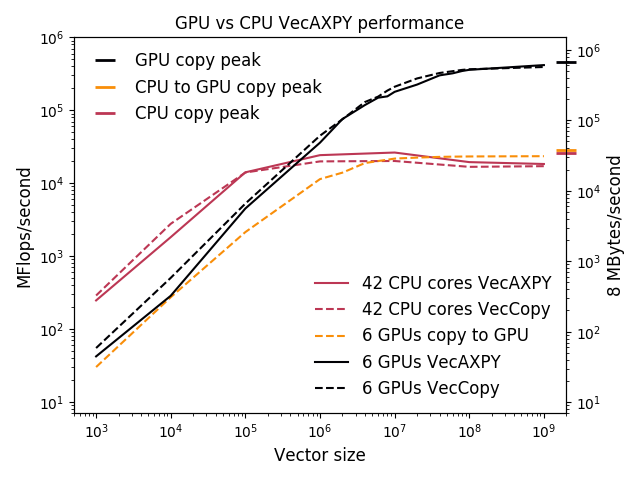
The benchmark code used is simple but exercises some basic building blocks common to many applications, and its simplicity allows us to construct analytical performance models that are useful for reasoning about more complicated scenarios. The code performs the following PETSc vector operations: VecAXPY, which computes , and VecCopy, which copies a vector via memcpy on the CPU and cudaMemcpy on the GPU or between the CPU and GPU. A single vector operation is timed for each operation. All vector sizes refer to the vector’s global size, spread among multiple computational units. There are two floating-point operations per entry for the VecAXPY operation. There are three memory accesses per vector entry for VecAXPY and two for VecCopy.
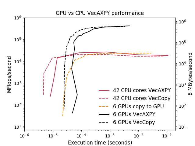
Figure 6 presents the memory throughput and VecAXPY performance observed on a node on a logarithmic scale. GPUs perform significantly better than the 42 CPU cores toward the right side of the graph, while CPUs are faster toward the left. The rightmost plot presents an alternative view of the same data, known as a static scaling or work-time spectrum plot [25, 26]. This view may appear confusing at first because the quantity being controlled (the vector size) does not appear on any of the plot axes, but it has the advantage that both the asymptotic bandwidth and the operations’ latency can be directly read. From the work-time spectrum plot, it is clear that the GPUs can deliver much higher memory bandwidth and throughput, while the CPUs offer much lower latency.
5.2 Communication operations with PetscSF
This section presents performance results for some simple PetscSF tests, related directly to Responses A2, A4, and A5. The first few tests are of Ping-Pong style between two MPI ranks. The last test represents communications in stencil computations with multiple MPI ranks. All tests use MPI_DOUBLE as the data type, and root/leaf data is allocated in GPU memory. Results shown here are an excerpt from a complete analysis, involving additional rank placements, given in [28].
5.2.1 Ping-pong tests
In a first test, sf_pingpong, we consider a star-forest with contiguous roots on rank 0 and contiguous leaves on rank 1, with leaf connecting to root for in . The test repeatedly calls PetscSFBcast and PetscSFReduce and mimics the OSU latency test from [29], which is commonly used to measure the latency of MPI sends and receives. No pack or unpack kernels or intermediate buffers are needed, and the root/leaf data is used directly in MPI calls. In a second test, called sf_unpack, we consider the same star forest but using the PetscSFBcastAndOp(..,op) and PetscSFReduce(..,op) API with op=MPI_SUM in the loop body, so that root values are added to leaves and vice versa. In this case, PetscSF needs to allocate a buffer on the receiver side and call an unpack kernel to sum the receive buffer data. The third test is called sf_scatter and considers additional leaves on rank 0, one for each root on the same rank. The test has the same loop body as sf_unpack. For this configuration, in PetscSFBcastAndOP rank 0 has to add root values to both local and remote leaves (on rank 1), while in PetscSFReduce both ranks contribute their leaf values to the roots on rank 0. Therefore, rank 0 has both local and remote communications. In local communications, it can directly scatter source data to destination data.
We tested the OSU latency test (osu_pingpong) and these three tests, all with GPU data, with two MPI ranks on two GPUs attached to the same CPU within a compute node. The average one-way latency results for the tests are shown in Table 1.
| Msg size(bytes) | 8K | 32K | 128K | 512K | 2M | 4M |
|---|---|---|---|---|---|---|
| osu_pingpong(s) | 17.8 | 17.8 | 20.0 | 28.2 | 61.7 | 106.6 |
| sf_pingpong(s) | 24.0 | 24.1 | 25.9 | 34.2 | 67.6 | 112.2 |
| sf_unpack(s) | 35.7 | 35.7 | 37.4 | 46.7 | 81.2 | 138.8 |
| sf_scatter(s) | 35.6 | 35.7 | 37.4 | 46.7 | 81.2 | 140.5 |
Timings for sf_pingpong are regularly 6 s larger than for osu_pingpong. Of these, 4 s is in cudaStreamSynchronize, around 1 s is spent on cudaPointerGetAttributes to get the memory types of the two data pointer arguments, and the software stack overhead of PetscSF is about 1 s. Compared with sf_pingpong, sf_unpack has an extra unpack kernel call after MPI_Waitall (ref. Figure 5(b)). For small messages (2 MB), sf_unpack timings are about 11 s larger than sf_pingpong, which is about a CUDA kernel launch cost. For large messages, kernel execution time becomes prominent. With sf_scatter, we add local communication with a bandwidth-limited kernel performing dst[i] += src[i]. For 4 MB of data, its execution time is about 14 s, including both read and write. Even including the kernel launch time, the local communication time is always smaller than the MPI Ping-Pong latency, which means that it is hidden by remote communication. The sf_scatter time is almost always equal to sf_unpack time except at 4 MB, where we hypothesize some memory system interference between MPI and the unpack kernel.
5.2.2 Stencil communication
We now consider communications in a 5-point stencil computation. We build a periodic 2D grid using PETSc DMDA over a processor grid and compare two different configurations for process placement: the first using nine compute nodes, each using one GPU per node, and the second using three compute nodes, each using three GPUs (all attached to the same CPU) per node. In both configurations, the GPUs are not shared among the MPI ranks. Work and communication loads are evenly distributed: for instance, with three nodes, each rank communicates with two intranode neighbors and two internode neighbors.
Each process owns a subgrid and has to communicate the values of the four sides of its subgrid with the corresponding neighbors. On each process, global vectors have a local length of , while local vectors have a length of , including ghost points along the four sides. DMGlobalToLocal updates local vectors from global vectors, while the reverse is done with DMLocalToGlobal. Both use PetscSF functionality under the hood. In this example, local communication involves the entire owned part of a global vector and the interior part (excluding ghost points) of a local vector, while remote communication involves packing and unpacking values along the four sides of a global vector and ghost points of a local vector. Because the indices for these values have a structured pattern, PetscSF can optimize the pack and unpack kernels and avoid copying the indices to GPUs.
| Subgrid size | 64 | 128 | 256 | 512 | 1024 | 2048 | 4096 |
|---|---|---|---|---|---|---|---|
| 9 nodes(s) | 45.0 | 46.0 | 46.3 | 47.1 | 57.1 | 139.9 | 499.9 |
| 3 nodes(s) | 75.8 | 75.9 | 75.9 | 76.0 | 83.0 | 139.0 | 498.3 |
Similar to the Ping-Pong tests, we call DMGlobalToLocal and DMLocalToGlobal in a loop and measure the average one-way latency, shown in Table 2. Latency remains constant with small subgrids () for both the nine-node and three-node configurations because remote communication hides local communication. Within this range of sizes, the nine-node configuration is faster because internode GPU MPI latency is smaller than intranode latency for messages 128 KB [28]. With larger subgrids, local communication costs (proportional to ) dominate remote communication cost (proportional to ); when , both configurations perform similarly since the difference in MPI remote communication time is hidden by the local communication time.
5.3 2D driven cavity with geometric multigrid
We examine the performance of the PETSc GPU infrastructure with the CUDA back-end on a straightforward application of geometric multigrid to a two-dimensional nonlinear lid-driven cavity benchmark in a velocity-vorticity formulation discretized by using a standard 5-point finite-difference stencil on a Cartesian structured mesh. PETSc’s built-in multigrid framework PCMG uses only front-end calls and can thus run entirely on the GPU in the solve phase by exploiting available optimized back-end kernels.
We use the PETSc SNES ex19 tutorial and employ Jacobi-preconditioned Chebyshev smoothers on all levels but the coarsest, where a redundant direct solver is executed on the CPU. An initial 44 grid is refined 10 times, resulting in a problem with 37.8 million degrees of freedom. The experiments reported here consider two types of multigrid cycles: a V-cycle, which begins at the finest level, visits each coarser level successively, and then incrementally returns up to the finest level, and a W-cycle, which begins by descending from the finest level to the coarsest as in a V-cycle but performs more sweeps on coarse levels, moving from fine to coarser levels during a gradual return to the finest level. In both cases, we use 9 levels of the multigrid hierarchy. Level 0 is the coarsest, and level 8 is the finest.
The results use 24 MPI ranks, since this number yields the fastest overall solution time, enabling sufficient use of the CPUs without incurring too much overhead from sharing the 6 GPUs For the problem studied here, the total solve times are equal when using V- or W-cycles when running on the CPU, but we examine both cases because of the importance of W-cycles for other problems and because the larger time spent on the coarser levels requires application of Response A3.
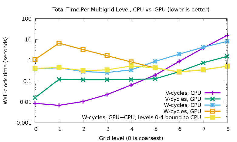
Figure 7 compares the time spent on each level of the multigrid solve for the CPU-only and GPU cases. For the V-cycle, the high latency for GPU operations is clear in the plateau between levels 1 to 5; although level 5 is 237 times larger than level 1, the time spent on the two levels is nearly identical. Instead, the CPU is capable of much lower-latency solves, and it is significantly faster than the GPU for levels 0–4. Because the bulk of the computational cost is on the finer levels, the total application time for the multigrid preconditioner on the GPU is 6.5 times faster than utilizing only the CPU. Running levels 0 to 4 on the CPU while using the GPU only on the expensive fine levels could produce a 10% performance improvement (details not shown).
With the W-cycle multigrid, the pure GPU solver is only 15% faster than the pure CPU solver, since the coarser levels are visited many more times than with the V-cycle. Again, by running levels 0 to 4 on the CPU, we avoid paying the high latency costs and achieve a speedup of 4.3 versus the pure CPU case. Note that the higher cost of level 4 is expected, since this includes data transfers between the GPU and CPU that must occur between levels 4 and 5. Although binding the coarse levels to the CPU significantly improves the performance of the W-cycle, this strategy should be combined with agglomeration of pieces of the coarse levels onto a smaller collection of MPI ranks so that Response A3 can be used. Support for such agglomeration currently exists in PETSc [30], and we will improve the multigrid infrastructure to make this happen in an automatic, GPU-aware way.
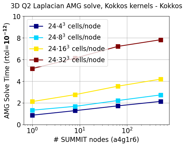
5.4 Algebraic multigrid on GPUs
Responses to F3 and A3 of performance portability is demonstrated by a scaling study with PETSc’s built-in algebraic multigrid (AMG) solver, PCGAMG, using cuSPARSE and Kokkos (with Kokkos Kernels) back-ends on our most mature device, CUDA (see Figure 2, upper left). Both solvers share the same MPI layer. PCGAMG uses the PCMG framework and can thus take advantage of optimized back-end operations. This ability to abstract the AMG algorithm with standard sparse linear algebra has facilitated its widespread use in the PETSc and wider computational science community. GPU implementations of parts of the setup phase of PCGAMG are under development, such as the maximal independent set algorithm for graph coarsening and the matrix triple product for coarse-grid construction.
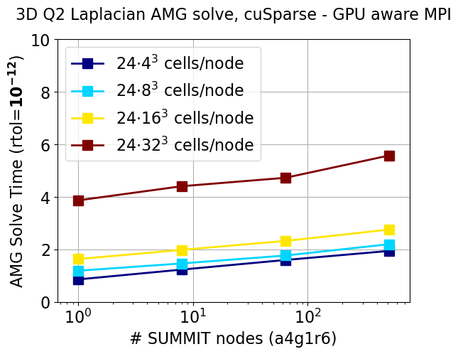
PETSc’s built-in FEM functionality is used to discretize the Laplacian operator with second-order elements. Each MPI process has a logical cube of hexahedral cells, with 24 such processes per node (i.e., 4 MPI tasks per GPU). Increasingly larger grids are generated by uniform refinements.
Figure 8 shows performance data for the solve phase with several subdomain sizes as a function of the number of nodes, keeping the same number of cells per MPI task, that is, weak scaling where horizontal lines are perfect. This shows that MPI parallel scaling is fairly good (there is a slight increase in iteration counts that is folded into the inefficiency) because the lines are almost flat, up to 512 nodes of Summit. The slower performance of Kokkos Kernels is due to PETSc’s explicitly computing a transpose for matrix transpose multiply, which Kokkos does not do. We note that Kokkos is faster when configured with using the cuSPARSE kernels (data not shown).
5.5 OpenFOAM: An application perspective
PETSc users often utilize only its Krylov solver infrastructure KSP, while managing time loops and nonlinear solution methods within the application. One example is OpenFOAM [31], and its solver plugin PETSc4FOAM [32], where matrices and vectors are computed on the CPU and passed to PETSc to solve the linear system.
To showcase the capabilities of the PETSc GPU solver infrastructure, we consider the time needed to perform twenty timesteps of a three-dimensional incompressible lid-driven cavity flow solver with a structured grid of 8 million cells [33]. The miniapp requires solving three momentum equations (one for each direction) and two pressure equations at each time step. Each momentum solve uses five iterations of BiCGstab preconditioned with block-diagonal ILU(0), while the pressure equations are solved to a relative tolerance of using the conjugate gradient method preconditioned with AMG. All PETSc solvers are set up on the CPU and run entirely on the GPU using the cuSPARSE back-end. The miniapp is run using one node from 1 MPI process with 1 GPU to 24 MPI processes and 4 GPUs, with a one-to-one mapping between MPI processes and GPU up to 6 MPI processes; when using 12 (resp. 24) processes, each GPU is shared by 2 (resp. 4) MPI processes.
Timing results are collected in Figure 9. In the upper left corner we compare the miniapp total time using the native OpenFOAM CPU solvers and the PETSc GPU solvers as a function of the number of processes in a log-log plot. The speedups range from 4 (with 1 MPI process) to 1.4 (with 24 processes). The two panels on the bottom row for the pressure equations (left) and the momentum equations (right), report timings for the various PETSc computational phases, namely, Mat for operator assembly, PC for preconditioner setup, and KSP for the Krylov method. Preconditioner setup runs on the CPU and tends to dominate the timings with larger local problems; however, these phases scale reasonably well with the number of CPU processes. On the other hand, the pure GPU phases of the Krylov methods scale well only up to 6 MPI processes (1 GPU each), and then computing times tend to increase with GPU oversubscription and smaller problem sizes. We expect improvements when the techniques highlighted in Response A3 will be fully implemented. Operators assembly only occupies a small fraction of the total time thanks to the optimized COO assembly routine MatSetValuesCOO that relates to Response A4. To quantify the benefits, in the upper-right corner, we provide a log-log plot of the timings using MatSetValuesCOO or the standard loop with MatSetValues.
 |
 |
 |
 |
5.6 Landau collision integral solver
We show progress on performance portability with an analysis of PETSc’s new Landau collision operator with two implementations of the CUDA programming model: CUDA and Kokkos. In collaboration with the WDMApp ECP project, we have deployed a Landau collision integral solver in PETSc [34]. This operator is wrapped in TS residual and Jacobian functions and uses standard algebraic solvers to provide an implicit time advance of the collision operator for kinetic plasma physics applications.
The Landau form of Fokker-Planck collisions is a velocity space operator and is the gold standard for fusion plasmas. The kernel is well suited to vector and GPU processing, and we have implemented CUDA and Kokkos versions of the GPU kernel. Our Landau operator uses the mesh adaptivity library p4est, used by the DMForest class. Adaptive meshes reduce the cost of resolving plasma distributions such as near Maxwellian distributions, which are concentrated at the origin, and the addition of fast alpha particles, which require that a larger velocity domain be resolved.
The Landau solver’s performance is tested on one node using one MPI process with one GPU. This test problem has 62 Q3 elements (992 integration points). Figure 10 shows the time for the construction of the Jacobian matrix, the GPU kernel, and the CPU matrix assembly and solve as a function of the number of species. Only the Landau kernel has been ported to the GPU. We observe that the times increase linearly with the number of species in the GPU kernel. This implies that the kernel is memory bound and not compute bound as the work increases quadratically with the number of species. The serial matrix assembly times increase quadratically. Porting the matrix assembly to the GPU is the subject of ongoing development.
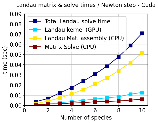
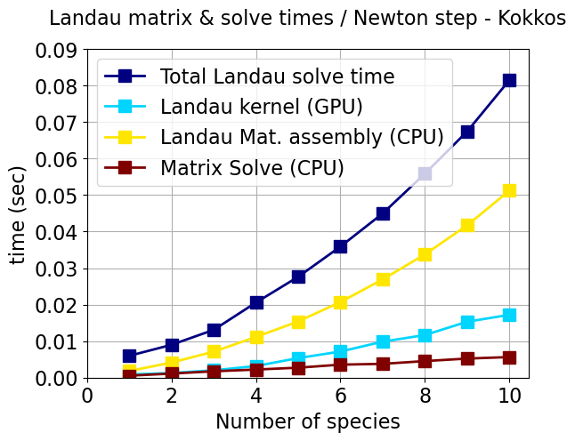
The Kokkos version is a little slower and required a rewrite of the Landau kernel to use a variable-length C++ 5D array (VLA) instead of a hardwired C array in the CUDA version, and the inner (third level of hierarchical parallelism in the algorithm) loop used a Kokkos parallel reduce instead of a manual parallel loop and reduce in the CUDA version. The VLA creates extra overhead in abstraction but benefits from a cleaner and more maintainable code. We are working with NVIDIA engineers to understand the performance of both GPU implementations.
6 Conclusion
This paper has explored and summarized our steady progress toward providing performance-portable high-throughput mathematical library support for GPUs. The back-end code is mostly completed for CUDA and Kokkos and roughly half-completed for HIP, and we are beginning to provide support for SYCL. In each case, we have utilized the corresponding mathematical libraries provided by third parties to leverage optimizations developed within the community. We have also provided a blueprint for adding performance-portable PETSc utilization to PETSc application codes. PETSc can now run complete algebraic solvers on the GPU, and we have begun developing on-device matrix assembly support, thus opening the door for PDE simulation applications to more completely utilize GPU-based exascale computing systems.
In addition, we have summarized the many technical challenges faced in utilizing GPUs in performance-portable libraries and the techniques PETSc uses to meet them. The key issue identified is the provision of an uninterrupted stream of instructions to the compute cores for highest possible data bandwidths on the GPUs or in combination with the CPUs. We have discussed how the organization of PETSc’s communication module and object management, in particular, will allow us to achieve exascale performance, and we have noted that no crucial outstanding technical problems remain.
Acknowledgments
This work was supported by the Exascale Computing Project (17-SC-20-SC), a collaborative effort of two US Department of Energy organizations (Office of Science and the National Nuclear Security Administration), responsible for the planning and preparation of a capable exascale ecosystem, including software, applications, hardware, advanced system engineering, and early testbed platforms, in support of the nation’s exascale computing imperative, and by the Austrian Science Fund (FWF) under grant P29119-N30. This research used resources of the Argonne and Oak Ridge Leadership Computing Facilities, DOE Office of Science User Facilities supported under Contracts DE-AC02-06CH11357 and DE-AC05-00OR22725, respectively.
References
- [1] S. Balay, S. Abhyankar, M. F. Adams, J. Brown, P. Brune, K. Buschelman, L. Dalcin, A. Dener, V. Eijkhout, W. D. Gropp, D. Karpeyev, D. Kaushik, M. G. Knepley, D. A. May, L. C. McInnes, R. T. Mills, T. Munson, K. Rupp, P. Sanan, B. F. Smith, S. Zampini, H. Zhang, H. Zhang, PETSc users manual, Tech. Rep. ANL-95/11 - Revision 3.13, Argonne National Laboratory, https://www.mcs.anl.gov/petsc (2020).
- [2] H. C. Edwards, C. R. Trott, D. Sunderland, Kokkos: Enabling manycore performance portability through polymorphic memory access patterns, Journal of Parallel and Distributed Computing 74 (12) (2014) 3202–3216, Domain-Specific Languages and High-Level Frameworks for High-Performance Computing. doi:10.1016/j.jpdc.2014.07.003.
- [3] D. A. Beckingsale, J. Burmark, R. Hornung, H. Jones, W. Killian, A. J. Kunen, O. Pearce, P. Robinson, B. S. Ryujin, T. R. Scogland, RAJA: Portable performance for large-scale scientific applications, in: 2019 IEEE/ACM International Workshop on Performance, Portability and Productivity in HPC (P3HPC), IEEE, 2019, pp. 71–81.
- [4] Khronos SYCL Working Group, SYCL specification: Generic heterogeneous computing for modern C++, https://www.khronos.org/-registry/SYCL/specs/sycl-2020-provisional.pdf (2020).
- [5] NVIDA, CUDA C++ programming guide, https://docs.nvidia.com/cuda/-pdf/CUDA_C_Programming_Guide.pdf (2020).
- [6] AMD, HIP programming guide, https://rocmdocs.amd.com/en/latest/-Programming_Guides/HIP-GUIDE.html (2020).
- [7] J. E. Stone, D. Gohara, G. Shi, OpenCL: A parallel programming standard for heterogeneous computing systems, Computing in science & engineering 12 (3) (2010) 66–73.
- [8] J. Brown, M. G. Knepley, D. A. May, L. C. McInnes, B. F. Smith, Composable linear solvers for multiphysics, in: Proceeedings of the 11th International Symposium on Parallel and Distributed Computing (ISPDC 2012), IEEE Computer Society, 2012, pp. 55–62.
- [9] J. Reinders, B. Ashbaugh, J. Brodman, M. Kinsner, J. Pennycook, X. Tian, Data parallel C++: Mastering DPC++ for programming of heterogeneous systems using C++ and SYCL (2020).
- [10] S. Pennycook, S. Hammond, S. Wright, J. Herdman, I. Miller, S. Jarvis, An investigation of the performance portability of OpenCL, Journal of Parallel and Distributed Computing 73 (11) (2013) 1439–1450.
- [11] N. Dryden, N. Maruyama, T. Moon, T. Benson, A. Yoo, M. Snir, B. Van Essen, Aluminum: An asynchronous, GPU-aware communication library optimized for large-scale training of deep neural networks on HPC systems, in: 2018 IEEE/ACM Machine Learning in HPC Environments (MLHPC), 2018, pp. 1–13. doi:10.1109/MLHPC.2018.8638639.
- [12] NVIDIA, NVIDIA collective communication library (NCCL) documentation, https://docs.nvidia.com/deeplearning/nccl/archives/nccl_278/user-guide/docs/index.html (2020).
- [13] NVIDIA, NVIDIA OpenSHMEM library (NVSHMEM) documentation, https://docs.nvidia.com/hpc-sdk/nvshmem/api/docs/introduction.html (2020).
- [14] Open Source Software Solutions, Inc., OpenSHMEM application programming interface v1.5, http://www.openshmem.org/ (2020).
- [15] S. Filippone, V. Cardellini, D. Barbieri, A. Fanfarillo, Sparse matrix-vector multiplication on GPGPUs, ACM Trans. Math. Softw. 43 (4) (Jan. 2017). doi:10.1145/3017994.
- [16] A. Haidar, S. Tomov, J. Dongarra, N. J. Higham, Harnessing GPU tensor cores for fast FP16 arithmetic to speed up mixed-precision iterative refinement solvers, in: SC18: International Conference for High Performance Computing, Networking, Storage and Analysis, IEEE, 2018, pp. 603–613.
- [17] O. Zachariadis, N. Satpute, J. Gómez-Luna, J. Olivares, Accelerating sparse matrix–matrix multiplication with GPU tensor cores, Computers & Electrical Engineering 88 (2020) 106848.
- [18] P. Blanchard, N. J. Higham, F. Lopez, T. Mary, S. Pranesh, Mixed precision block fused multiply-add: Error analysis and application to GPU tensor cores, SIAM Journal on Scientific Computing 42 (3) (2020) C124–C141.
- [19] V. Minden, B. F. Smith, M. G. Knepley, Preliminary implementation of PETSc using GPUs, in: D. A. Yuen, L. Wang, X. Chi, L. Johnsson, W. Ge, Y. Shi (Eds.), GPU Solutions to Multi-scale Problems in Science and Engineering, Lecture Notes in Earth System Sciences, Springer Berlin Heidelberg, 2013, pp. 131–140. doi:10.1007/978-3-642-16405-7_7.
- [20] H. Anzt, E. Boman, R. Falgout, P. Ghysels, M. Heroux, X. Li, L. Curfman McInnes, R. Tran Mills, S. Rajamanickam, K. Rupp, et al., Preparing sparse solvers for exascale computing, Philosophical Transactions of the Royal Society A 378 (2166) (2020) 20190053.
- [21] K. Rupp, P. Tillet, F. Rudolf, J. Weinbub, A. Morhammer, T. Grasser, A. Jungel, S. Selberherr, ViennaCL—linear algebra library for multi-and many-core architectures, SIAM Journal on Scientific Computing 38 (5) (2016) S412–S439.
- [22] P. Jolivet, J. E. Roman, S. Zampini, KSPHPDDM and PCHPDDM: Extending PETSc with robust overlapping Schwarz preconditioners and advanced Krylov methods, Computers & Mathematics with Applications 84 (2021) 277–295. doi:10.1016/j.camwa.2021.01.003.
- [23] J. Zhang, J. Brown, S. Balay, J. Faibussowitsch, M. Knepley, O. Marin, R. T. Mills, T. Munson, B. F. Smith, S. Zampini, The PetscSF scalable communication layer, IEEE Transactions on Parallel & Distributed Systems (2021). doi:10.1109/TPDS.2021.3084070.
- [24] F. G. Van Zee, D. N. Parikh, R. A. van de Geijn, Supporting mixed-domain mixed-precision matrix multiplication within the BLIS framework, ACM Transactions on Mathematical Software 47 (2) (2021). doi:10.1145/3402225.
- [25] J. Chang, K. Nakshatrala, M. G. Knepley, L. Johnsson, A performance spectrum for parallel computational frameworks that solve PDEs, Concurrency and Computation: Practice and Experience 30 (11) (2018) e4401.
- [26] J. Chang, M. S. Fabien, M. G. Knepley, R. T. Mills, Comparative study of finite element methods using the time-accuracy-size (TAS) spectrum analysis, SIAM Journal on Scientific Computing 40 (6) (2018) C779–C802.
- [27] H. M. Morgan, R. T. Mills, B. Smith, Evaluation of PETSc on a heterogeneous architecture, the OLCF Summit system: Part I: Vector node performance, Tech. Rep. ANL-19/41, Argonne National Laboratory (2020). doi:10.2172/1614879.
- [28] J. Zhang, R. T. Mills, B. F. Smith, Evaluation of PETSc on a heterogeneous architecture, the OLCF Summit system: Part II: Basic communication performance, Tech. Rep. ANL-20/76, Argonne National Laboratory (2020).
- [29] D. Panda, et al., OSU microbenchmarks v5.6.2, http://mvapich.cse.ohio-state.edu/benchmarks/ (2019).
- [30] D. A. May, P. Sanan, K. Rupp, M. G. Knepley, B. F. Smith, Extreme-scale multigrid components within PETSc, in: Proceedings of the Platform for Advanced Scientific Computing Conference, PASC ’16, Association for Computing Machinery, New York, NY, USA, 2016, pp. 1–12.
- [31] The OpenFOAM Foundation, OpenFOAM, https://openfoam.org/ (2020).
- [32] S. Bna, M. Olesen, S. Zampini, PETSc4FOAM, https://develop.openfoam.com/modules/external-solver (2020).
- [33] OpenFOAM HPC benchmark suite: 3D lid driven cavity flow, https://develop.openfoam.com/committees/hpc/-/tree/develop/Lid_driven_cavity-3d/M (2020).
- [34] M. F. Adams, E. Hirvijoki, M. G. Knepley, J. Brown, T. Isaac, R. Mills, Landau collision integral solver with adaptive mesh refinement on emerging architectures, SIAM Journal on Scientific Computing 39 (6) (2017) C452–C465. doi:10.1137/17M1118828.
The submitted manuscript has been created by UChicago Argonne, LLC, Operator of Argonne National Laboratory (“Argonne”). Argonne, a US Department of Energy Office of Science laboratory, is operated under Contract No. DE-AC02-06CH11357. The US Government retains for itself, and others acting on its behalf, a paid-up nonexclusive, irrevocable worldwide license in said article to reproduce, prepare derivative works, distribute copies to the public, and perform publicly and display publicly, by or on behalf of the Government. The Department of Energy will provide public access to these results of federally sponsored research in accordance with the DOE Public Access Plan. http://energy.gov/downloads/doe-public-accessplan