Toward Guidance-Free AR Visual Generation via Condition Contrastive Alignment
Abstract
Classifier-Free Guidance (CFG) is a critical technique for enhancing the sample quality of visual generative models. However, in autoregressive (AR) multi-modal generation, CFG introduces design inconsistencies between language and visual content, contradicting the design philosophy of unifying different modalities for visual AR. Motivated by language model alignment methods, we propose Condition Contrastive Alignment (CCA) to facilitate guidance-free AR visual generation with high performance and analyze its theoretical connection with guided sampling methods. Unlike guidance methods that alter the sampling process to achieve the ideal sampling distribution, CCA directly fine-tunes pretrained models to fit the same distribution target. Experimental results show that CCA can significantly enhance the guidance-free performance of all tested models with just one epoch of fine-tuning (1% of pretraining epochs) on the pretraining dataset, on par with guided sampling methods. This largely removes the need for guided sampling in AR visual generation and cuts the sampling cost by half. Moreover, by adjusting training parameters, CCA can achieve trade-offs between sample diversity and fidelity similar to CFG. This experimentally confirms the strong theoretical connection between language-targeted alignment and visual-targeted guidance methods, unifying two previously independent research fields. Code and model weights: https://github.com/thu-ml/CCA.
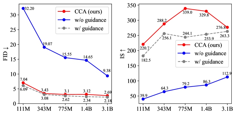
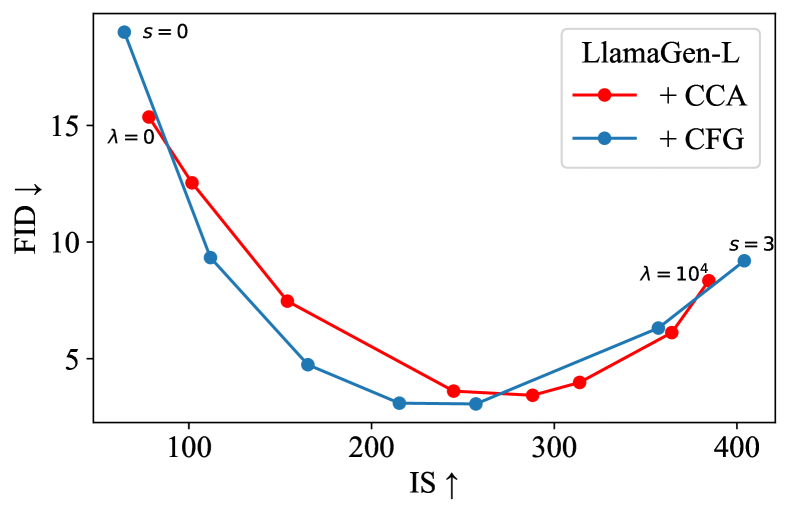
(a) LlamaGen
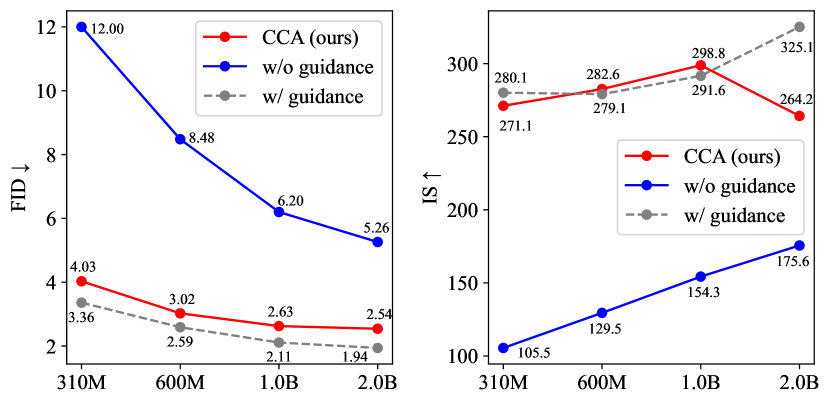
(b) VAR
1 Introduction
Witnessing the scalability and generalizability of autoregressive (AR) models in language domains, recent works have been striving to replicate similar success for visual generation (Esser et al., 2021; Lee et al., 2022). By quantizing images into discrete tokens, AR visual models can process images using the same next-token prediction approach as Large Language Models (LLMs). This approach is attractive because it provides a potentially unified framework for vision and language, promoting consistency in reasoning and generation across modalities (Team, 2024; Xie et al., 2024).
Despite the design philosophy of maximally aligning visual modeling with language modeling methods, AR visual generation still differs from language generation in a notable aspect. AR visual generation relies heavily on Classifier-Free Guidance (CFG) (Ho & Salimans, 2022), a sampling technique unnecessary for language generation, which has caused design inconsistencies between the two types of content. During sampling, while CFG helps improve sample quality by contrasting conditional and unconditional models, it requires two model inferences per visual token, which doubles the sampling cost. During training, CFG requires randomly masking text conditions to learn the unconditional distribution, preventing the simultaneous training of text tokens (Team, 2024).
In contrast to visual generation, LLMs rarely rely on guided sampling. Instead, the surge of LLMs’ instruction-following abilities has largely benefited from fine-tuning-based alignment methods (Schulman et al., 2022). Motivated by this observation, we seek to study: “Can we avoid guided sampling in AR visual generation, but attain similar effects by directly fine-tuning pretrained models?”
In this paper, we derive Condition Contrastive Alignment (CCA) for enhancing visual AR performance without guided sampling. Unlike CFG which necessitates altering the sampling process to achieve a more desirable sampling distribution, CCA directly fine-tunes pretrained AR models to fit the same distribution target, leaving the sampling scheme untouched. CCA is quite convenient to use since it does not rely on any additional datasets beyond the pretraining data. Our method functions by contrasting positive and negative conditions for a given image, which can be easily created from the existing pretraining dataset as matched or mismatched image-condition pairs. CCA is also highly efficient given its fine-tuning nature. We observe that our method achieves ideal performance within just one training epoch, indicating negligible computational overhead (1% of pretraining).
In Sec. 4, we highlight a theoretical connection between CCA and guided sampling techniques (Dhariwal & Nichol, 2021; Ho & Salimans, 2022). Essentially these methods all target at the same sampling distribution. The distributional gap between this target distribution and pretrained models is related to a physical quantity termed conditional residual (). Guidance methods typically train an additional model (e.g., unconditional model or classifier) to estimate this quantity and enhance pretrained models by altering their sampling process. Contrastively, CCA follows LLM alignment techniques (Rafailov et al., 2023; Chen et al., 2024a) and parameterizes the conditional residual with the difference between our target model and the pretrained model, thereby directly training a sampling model. This analysis unifies language-targeted alignment and visual-targeted guidance methods, bridging the gap between the two previously independent research fields.
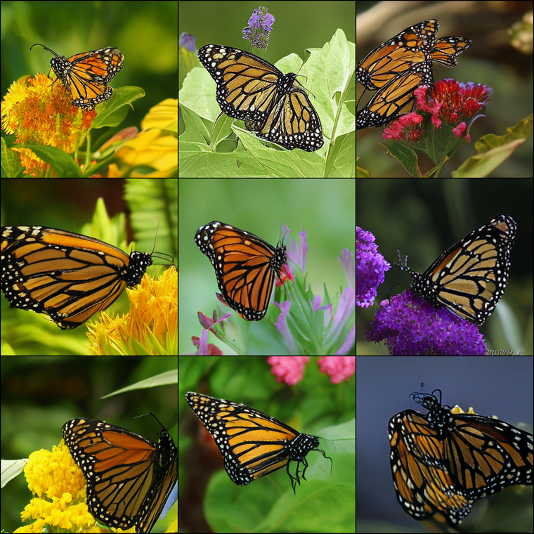
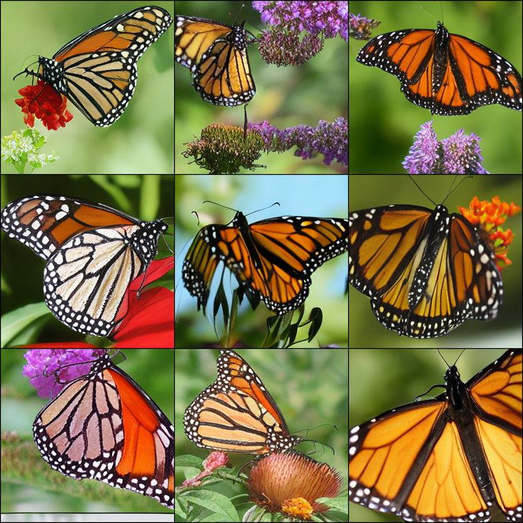
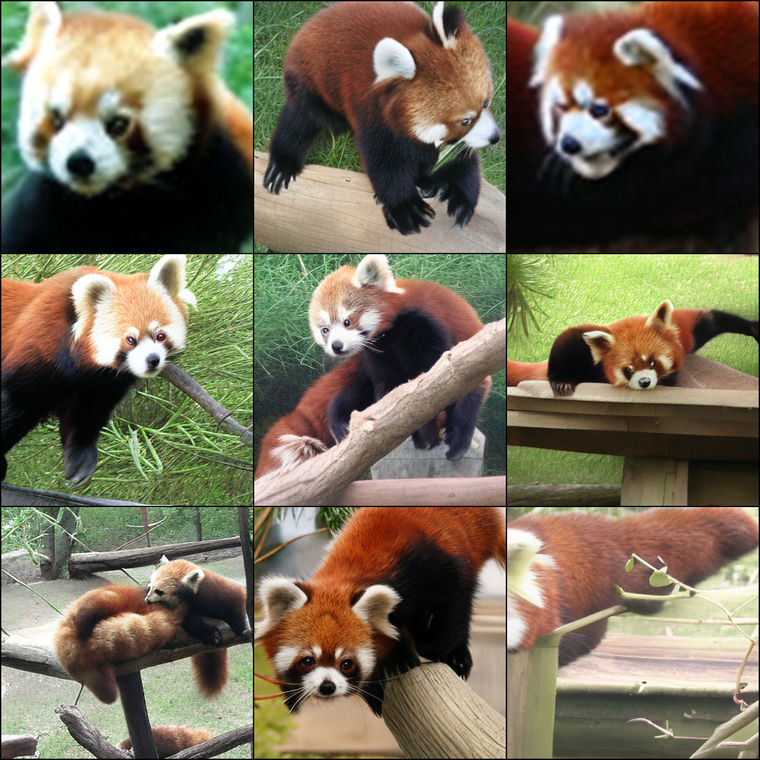
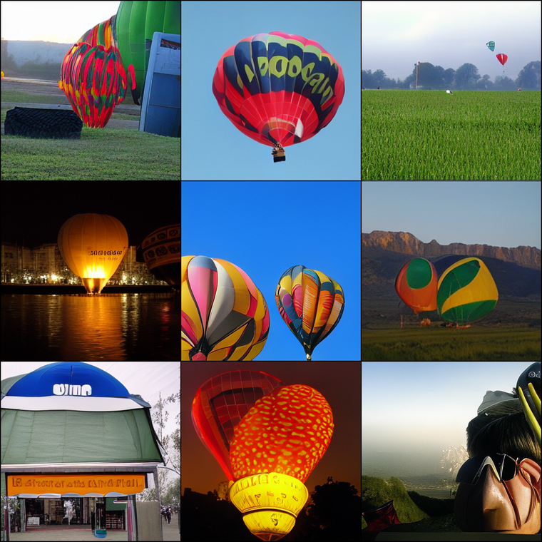
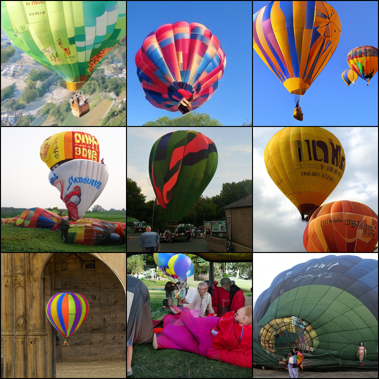
We apply CCA to two state-of-the-art autoregressive (AR) visual models, LLamaGen (Sun et al., 2024) and VAR (Tian et al., 2024), which feature distinctly different visual tokenization designs. Both quantitative and qualitative results show that CCA significantly and consistently enhances the guidance-free sampling quality across all tested models, achieving performance levels comparable to CFG (Figure 1). We further show that by varying training hyperparameters, CCA can realize a controllable trade-off between image diversity and fidelity similar to CFG. This further confirms their theoretical connections. We also compare our method with some existing LLM alignment methods (Welleck et al., 2019; Rafailov et al., 2023) to justify its algorithm design. Finally, we demonstrate that CCA can be combined with CFG to further improve performance.
Our contributions: 1. We take a big step toward guidance-free visual generation by significantly improving the visual quality of AR models. 2. We reveal a theoretical connection between alignment and guidance methods. This shows that language-targeted alignment can be similarly applied to visual generation and effectively replace guided sampling, closing the gap between these two fields.
2 Background
2.1 Autoregressive (AR) Visual Models
Autoregressive models.
Consider data represented by a sequence of discrete tokens , where each token is an integer. Data probability can be decomposed as:
| (1) |
AR models thus aim to learn , where each token is conditioned only on its previous input . This is known as next-token prediction (Radford et al., 2018).
Visual tokenization.
Image pixels are continuous values, making it necessary to use vector-quantized tokenizers for applying discrete AR models to visual data (Van Den Oord et al., 2017; Esser et al., 2021). These tokenizers are trained to encode images into discrete token sequences and decode them back by minimizing reconstruction losses. In our work, we utilize pretrained and frozen visual tokenizers, allowing AR models to process images similarly to text.
2.2 Guided Sampling for Visual Generation
Despite the core motivation of developing a unified model for language and vision, the AR sampling strategies for visual and text contents differ in one key aspect: AR visual generation necessitates a sampling technique named Classifier-Free Guidance (CFG) (Ho & Salimans, 2022). During inference, CFG adjusts the sampling logits for each token as:
| (2) |
where and are the conditional and unconditional logits provided by two separate AR models, and . The condition can be class labels or text captions, formalized as prompt tokens. The scalar is termed guidance scale. Since token logits represent the (unnormalized) log-likelihood in AR models, Ho & Salimans (2022) prove that the sampling distribution satisfies:
| (3) |
At , the sampling model becomes exactly the pretrained conditional model . However, previous works (Ho & Salimans, 2022; Podell et al., 2023; Chang et al., 2023; Sun et al., 2024) have widely observed that an appropriate is critical for an ideal trade-off between visual fidelity and diversity, making training another unconditional model necessary. In practice, the unconditional model usually shares parameters with the conditional one, and can be trained concurrently by randomly dropping condition prompts during training.
2.3 Direct Preference Optimization for Language Model Alignment
Reinforcement Learning from Human Feedback (RLHF) is crucial for enhancing the instruction-following ability of pretrained Language Models (LMs) (Schulman et al., 2022; OpenAI, 2023). Performing RL typically requires a reward model, which can be learned from human preference data. Formally, the Bradley-Terry preference model (Bradley & Terry, 1952) assumes.
| (4) |
where and are respectively the winning and losing response for an instruction , evaluated by human. represents an implicit reward for each response. The target LM should satisfy to attain higher implicit reward compared with the pretrained LM .
Direct Preference Optimization (Rafailov et al., 2023) allows us to directly optimize pretrained LMs on preference data, by formalizing :
| (5) |
DPO is more streamlined and thus often more favorable compared with traditional two-stage RLHF pipelines: first training reward models, then aligning LMs with reward models using RL.
3 Condition Contrastive Alignment
Autoregressive visual models are essentially learning a parameterized model to approximate the standard conditional image distribution . Guidance algorithms shift the sampling policy away from according to Sec. 2.2:
| (6) |
At guidance scale , sampling from is most straightforward. However, it is widely observed that an appropriate usually leads to significantly enhanced sample quality. The cost is that we rely on an extra unconditional model for sampling. This doubles the sampling cost and causes an inconsistent training paradigm with language.
In this section, we derive a simple approach to directly model the same target distribution by fine-tuning pretrained models. Specifically, our methods leverage a singular loss function for optimizing to become . Despite having similar effects as guided sampling, our approach does not require altering the sampling process. We theoretically derive our method in Sec. 3.1 and discuss its practical implementation in Sec. 3.2.
3.1 Algorithm Derivation
The core difficulty of directly learning is that we cannot access datasets under the distribution of . However, we observe the distributional difference between and is related to a simple quantity that can be potentially learned from existing datasets. Specifically, by taking the logarithm of both sides in Eq. 6 and applying some algebra, we have111We ignore a normalizing constant in Eq. 7 for brevity. A more detailed discussion is in Appendix B.:
| (7) |
of which the right-hand side (i.e., ) corresponds to the log gap between the conditional probability and unconditional probability for an image , which we term as conditional residual.
Our key insight here is that the conditional residual can be directly learned through contrastive learning approaches (Gutmann & Hyvärinen, 2012), as sated below:
Theorem 3.1 (Noise Contrastive Estimation, proof in Appendix A).
Let be a parameterized model which takes in an image-condition pair and outputs a scalar value . Consider the loss function:
| (8) |
Given unlimited model expressivity for , the optimal solution for minimizing satisfies
| (9) |
Now that we have a tractable way of learning , the target distribution can be jointly defined by and the pretrained model . However, we would still lack an explicitly parameterized model if is another independent network. To address this problem, we draw inspiration from the widely studied alignment techniques in language models (Rafailov et al., 2023) and parameterize with our target model and according to Eq. 7:
| (10) |
Then, the loss function becomes
| (11) |
During training, is learnable while pretrained is frozen. can be initialized from .
This way we can fit with a single AR model , eliminating the need for training a separate unconditional model for guided sampling. Sampling strategies for are consistent with standard language model decoding methods, which unifies decoding systems for multi-modal generation.
3.2 Practical Algorithm
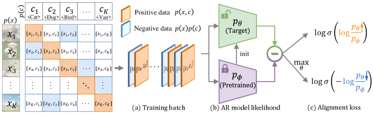
Figure 2 illustrates the CCA method. Specifically, implementing Eq. 11 requires approximating two expectations: one under the joint distribution and the other under the product of its two marginals . The key difference between these distributions is that in , images and conditions are correctly paired. In contrast, and are sampled independently from , meaning they are most likely mismatched.
In practice, we rely solely on the pretraining dataset to estimate . Consider a batch of data pairs . We randomly shuffle the condition batch to become , where each represents a negative condition of image , while the original is a positive one. This results in our training batch . The loss function is
| (12) |
where and are two hyperparameters that can be adjusted. replaces the guidance scale parameter , while is for controlling the loss weight assigned to negative conditions. The learnable is initialized from the pretrained conditional model , making a fine-tuning loss.
We give an intuitive understanding of Eq. 12. Note that is monotonically increasing. The first term of Eq. 12 aims to increase the likelihood of an image given a positive condition, with a similar effect to maximum likelihood training. For mismatched image-condition data, the second term explicitly minimizes its relative model likelihood compared with the pretrained .
We name the above training technique Condition Contrastive Alignment (CCA) due to its contrastive nature in comparing positive and negative conditions with respect to a single image. This naming also reflects its theoretical connection with Noise Contrastive Estimation (Theorem 3.1).
4 Connection between CCA and guidance methods
As summarized in Table 1, the key distinction between CCA and guidance methods is how to model , which defines the distributional gap between the target and (Eq. 7).
In particular, Classifier Guidance (Dhariwal & Nichol, 2021) leverages Bayes’ Rule and turn into a conditional posterior:
where is explicitly modeled by a classifier , which is trained by a standard classification loss. is regarded as a uniform distribution. CFG trains an extra unconditional model to estimate the unknown part of :
Despite their effectiveness, guidance methods all require learning a separate model and a modified sampling process compared with standard autoregressive decoding. In comparison, CCA leverages Eq. 7 and models as
which allows us to directly learn instead of another guidance network.
Although CCA and conventional guidance techniques have distinct modeling methods, they all target at the same sampling distribution and thus have similar effects in visual generation. For instance, we show in Sec. 5.2 that CCA offers a similar trade-off between sample diversity and fidelity to CFG.
Method Classifier Guidance Classifier-Free Guidance Condition Contrastive Alignment Modeling of Training loss in Eq. 11 Sampling policy Extra training cost 9% of learning 10% of learning 1% of pretraining Sampling cost 1.3 2 1 Applicable area Diffusion Diffusion & Autoregressive Autoregressive
5 Experiments
We seek to answer the following questions through our experiments:
-
1.
How effective is CCA in enhancing the guidance-free generation quality of pretrained AR visual models, quantitatively and qualitatively? (Sec. 5.1)
-
2.
Does CCA allow controllable trade-offs between sample diversity (FID) and fidelity (IS) similar to CFG? (Sec. 5.2)
-
3.
How does CCA perform in comparison to alignment algorithms for LLMs? (Sec. 5.3)
-
4.
Can CCA be combined with CFG to further improve performance? (Sec. 5.4)
5.1 Toward Guidance-Free AR Visual Generation
| Model | w/o Guidance | w/ Guidance | |||||
| FID | IS | Precision | Recall | FID | IS | ||
| Diffusion | ADM (Dhariwal & Nichol, 2021) | 7.49 | 127.5 | 0.72 | 0.63 | 3.94 | 215.8 |
| LDM-4 (Rombach et al., 2022) | 10.56 | 103.5 | 0.71 | 0.62 | 3.60 | 247.7 | |
| U-ViT-H/2 (Bao et al., 2023) | – | – | – | – | 2.29 | 263.9 | |
| DiT-XL/2 (Peebles & Xie, 2023) | 9.62 | 121.5 | 0.67 | 0.67 | 2.27 | 278.2 | |
| MDTv2-XL/2 (Gao et al., 2023) | 5.06 | 155.6 | 0.72 | 0.66 | 1.58 | 314.7 | |
| Mask | MaskGIT (Chang et al., 2022) | 6.18 | 182.1 | 0.80 | 0.51 | – | – |
| MAGVIT-v2 (Yu et al., 2023) | 3.65 | 200.5 | – | – | 1.78 | 319.4 | |
| MAGE (Li et al., 2023) | 6.93 | 195.8 | – | – | – | – | |
| Autoregressive | VQGAN (Esser et al., 2021) | 15.78 | 74.3 | – | – | 5.20 | 280.3 |
| ViT-VQGAN (Yu et al., 2021) | 4.17 | 175.1 | – | – | 3.04 | 227.4 | |
| RQ-Transformer (Lee et al., 2022) | 7.55 | 134.0 | – | – | 3.80 | 323.7 | |
| LlamaGen-3B (Sun et al., 2024) | 9.38 | 112.9 | 0.69 | 0.67 | 2.18 | 263.3 | |
| CCA (Ours) | 2.69 | 276.8 | 0.80 | 0.59 | – | – | |
| VAR-d30 (Tian et al., 2024) | 5.25 | 175.6 | 0.75 | 0.62 | 1.92 | 323.1 | |
| CCA (Ours) | 2.54 | 264.2 | 0.83 | 0.56 | – | – | |
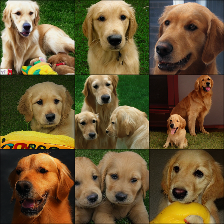
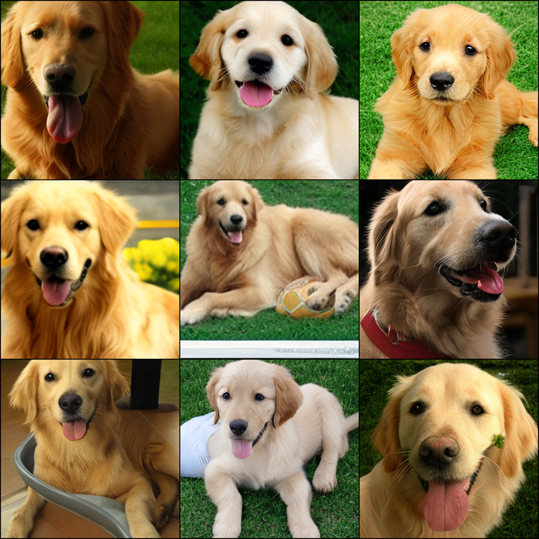
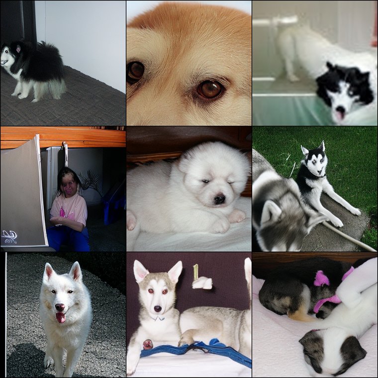
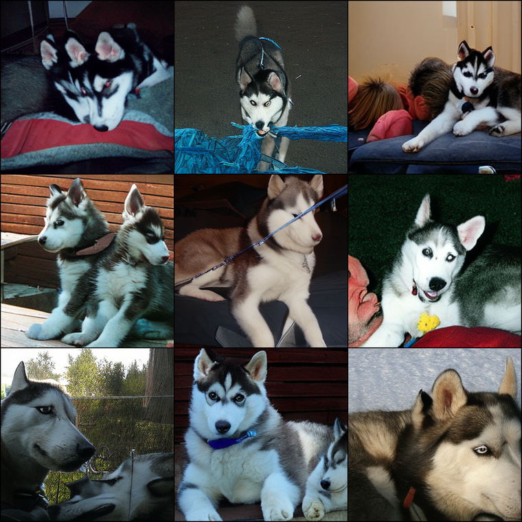
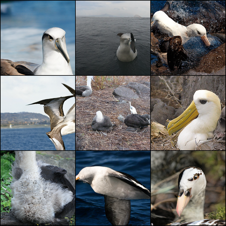
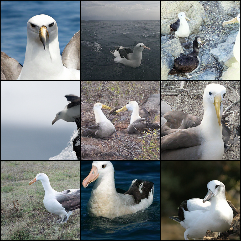
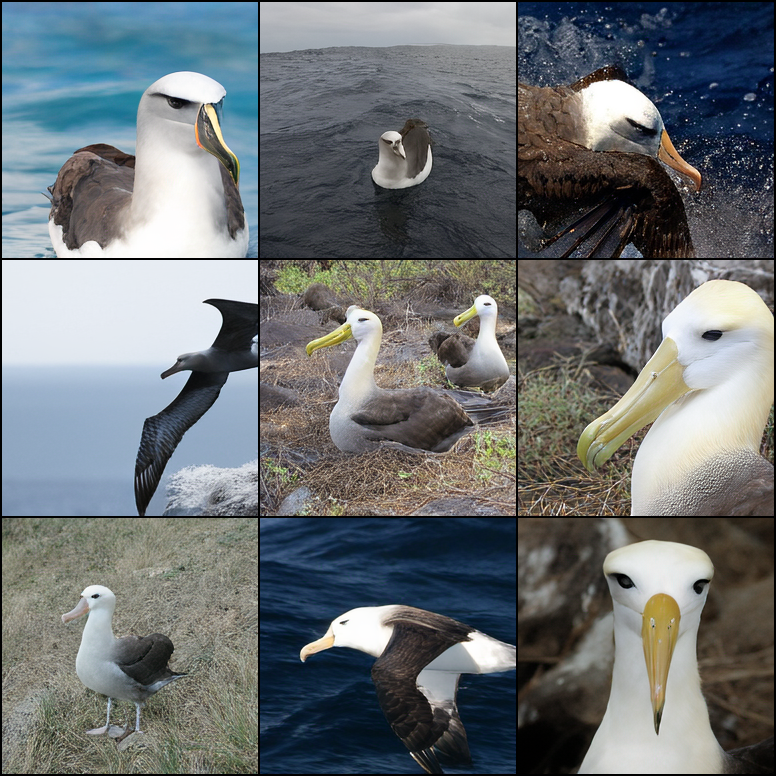
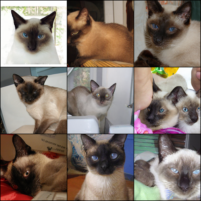
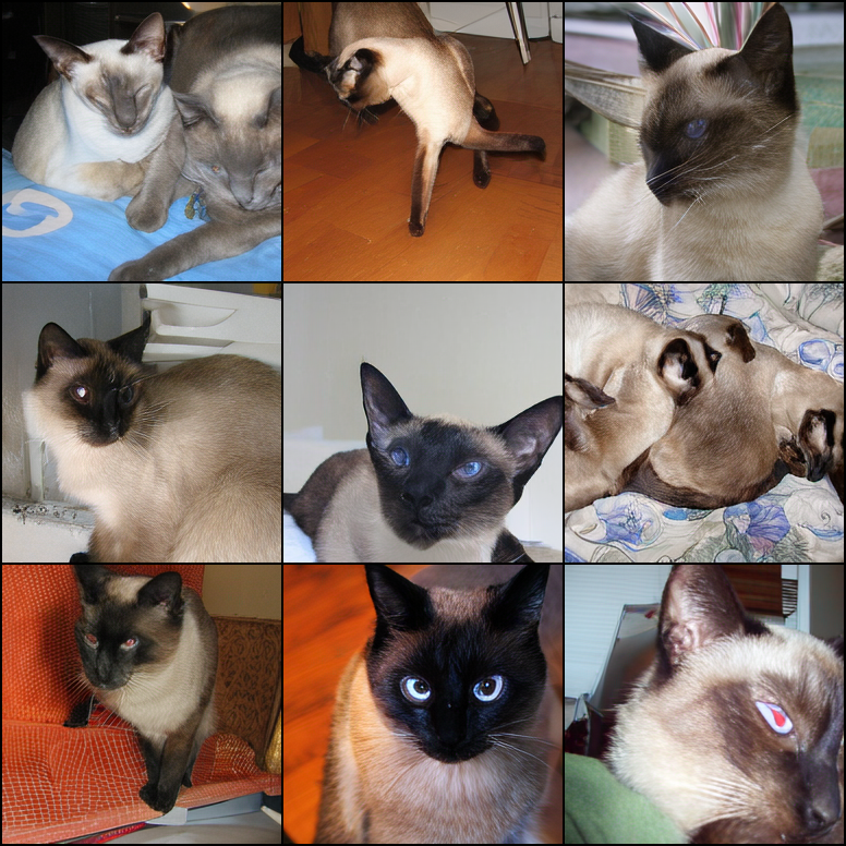
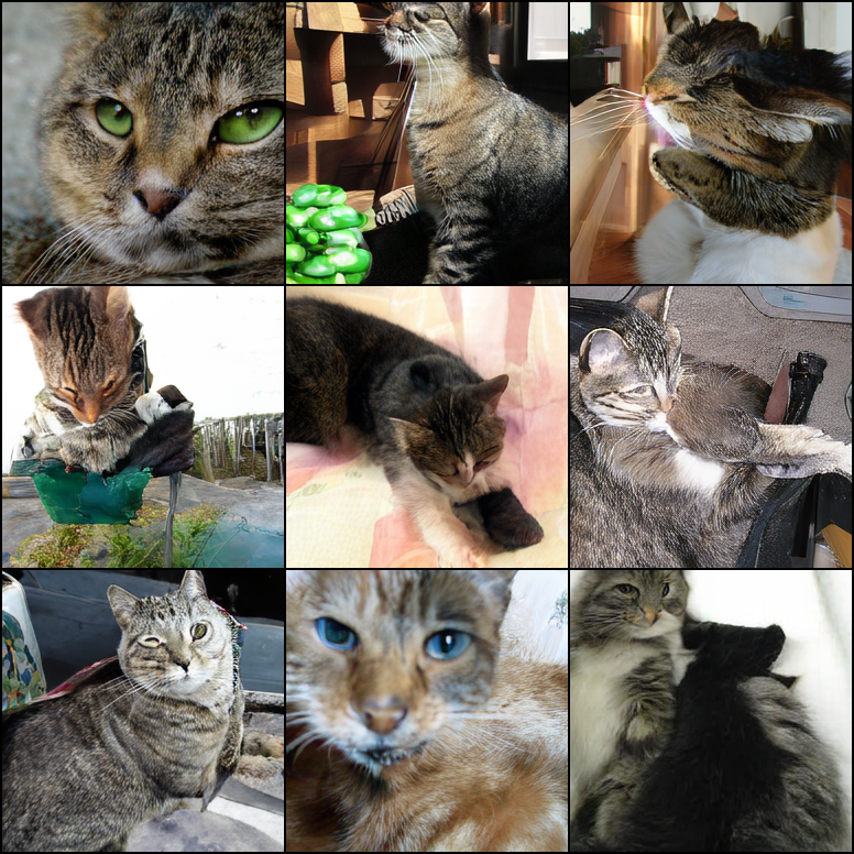
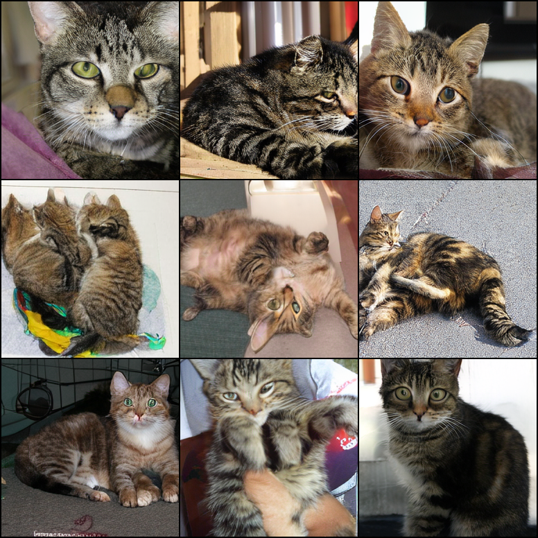
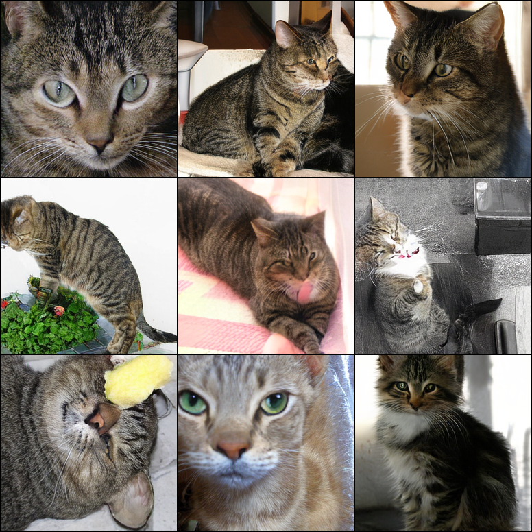
LlamaGen (w/o Guidance)
LlamaGen + CCA (w/o G.)
LlamaGen (w/ CFG)
IS=64.7
IS=384.6
IS=404.0
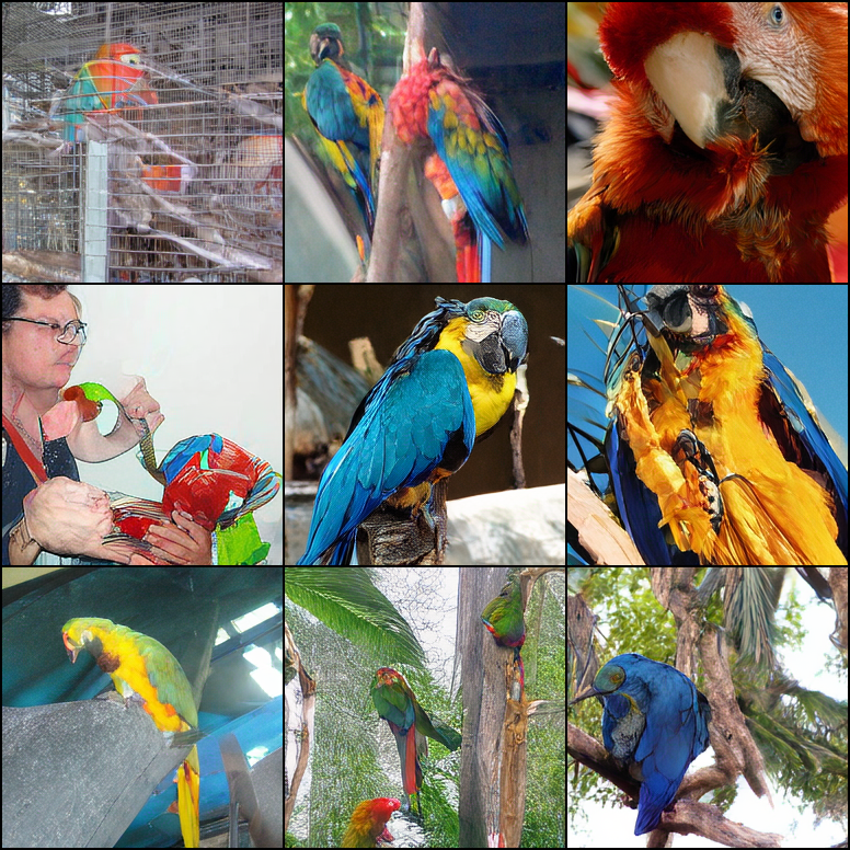
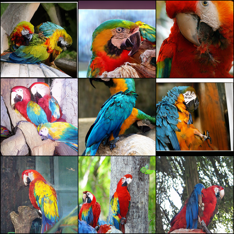
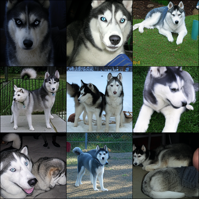
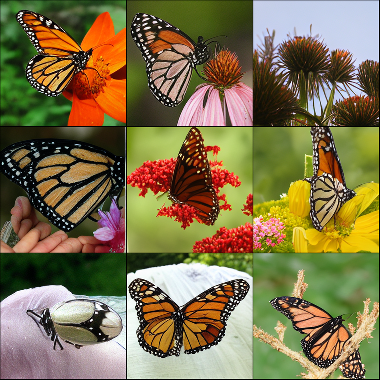
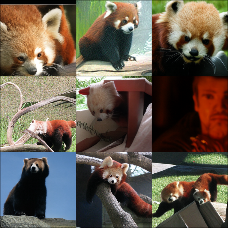
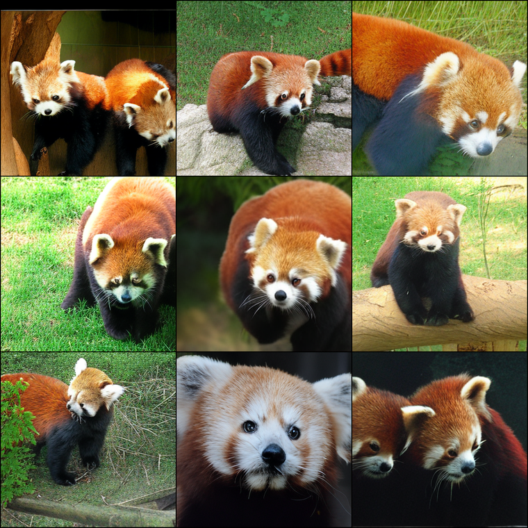
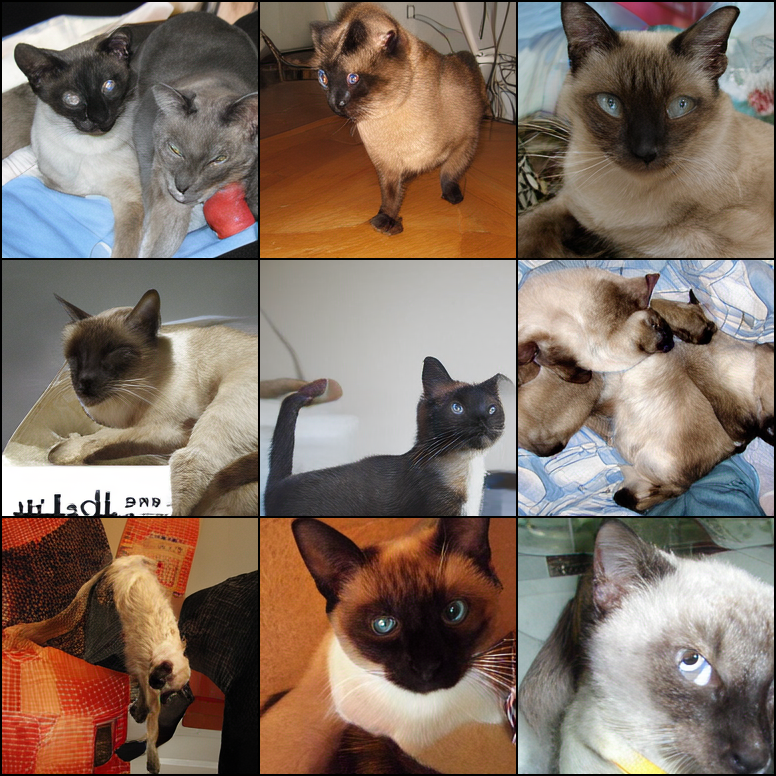
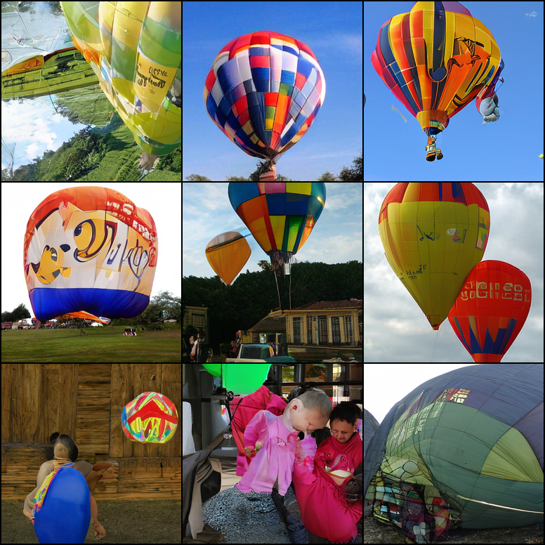
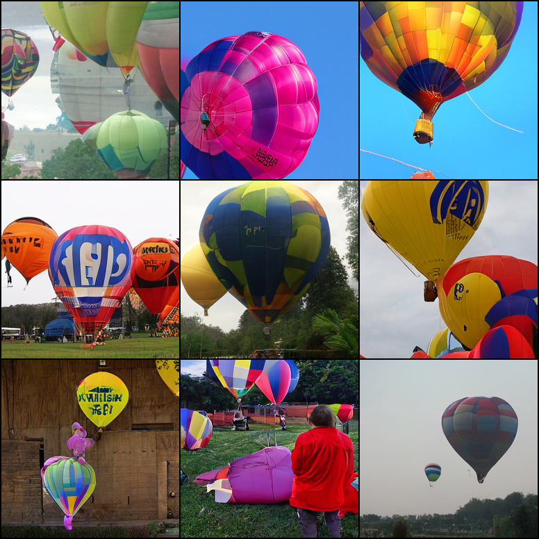
VAR (w/o Guidance)
VAR + CCA (w/o G.)
VAR (w/ CFGv2)
IS=154.3
IS=350.4
IS=390.8
Base model.
We experiment on two families of publicly accessible AR visual models, LlamaGen (Sun et al., 2024) and VAR (Tian et al., 2024). Though both are class-conditioned models pretrained on ImageNet, LlamaGen and VAR feature distinctively different tokenizer and architecture designs. LlamaGen focuses on reducing the inductive biases on visual signals. It tokenizes images in the classic raster order and adopts almost the same LLM architecture as Llama (Touvron et al., 2023a). VAR, on the other hand, leverages the hierarchical structure of images and tokenizes them in a multi-scale, coarse-to-fine manner. VAR adopts a GPT-2 architecture but tailors the attention mechanism specifically for visual content. For both works, CFG is a default and critical technique.
Training setup.
We leverage CCA to finetune multiple LlamaGen and VAR models of various sizes on the standard ImageNet dataset. The training scheme and hyperparameters are mostly consistent with the pretraining phase. We report performance numbers after only one training epoch and find this to be sufficient for ideal performance. We fix in Eq. 12 and select suitable for each model. Image resolutions are for LlamaGen and for VAR. Following the original work, we resize LlamaGen samples to whenever required for evaluation.
Experimental results.
We find CCA significantly improves the guidance-free performance of all tested models (Figure 1), evaluated by metrics like FID (Heusel et al., 2017) and IS (Salimans et al., 2016). For instance, after one epoch of CCA fine-tuning, the FID score of LlamaGen-L (343M) improves from 19.07 to 3.41, and the IS score from 64.3 to 288.2, achieving performance levels comparable to CFG. This result is compelling, considering that CCA has negligible fine-tunning overhead compared with model pretraining and only half of sampling costs compared with CFG.
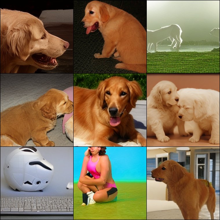
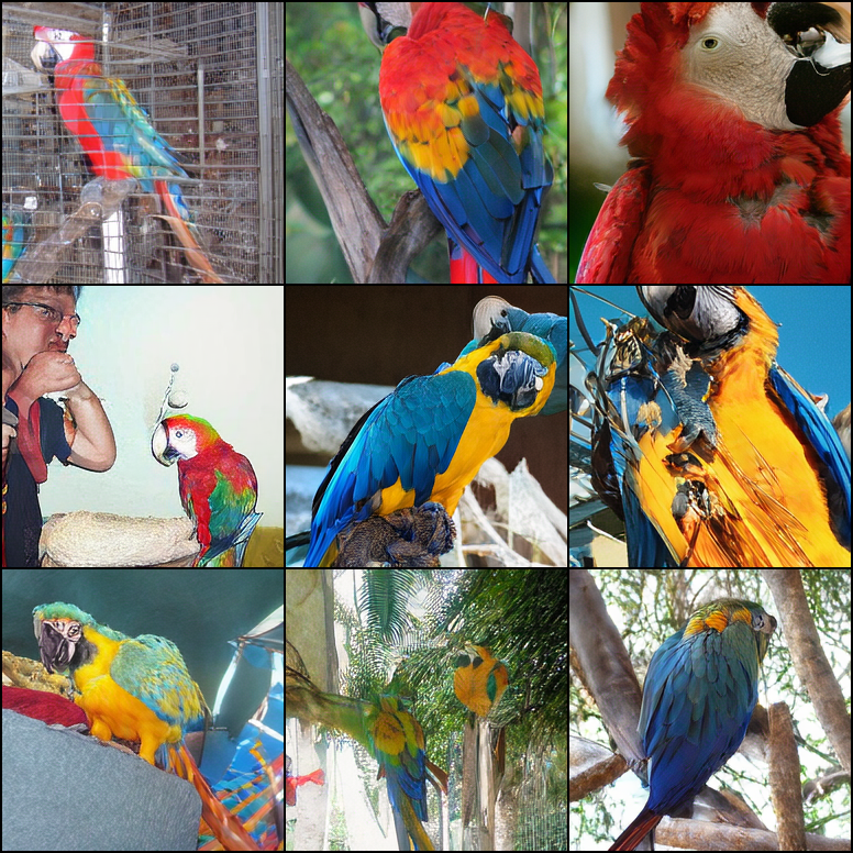
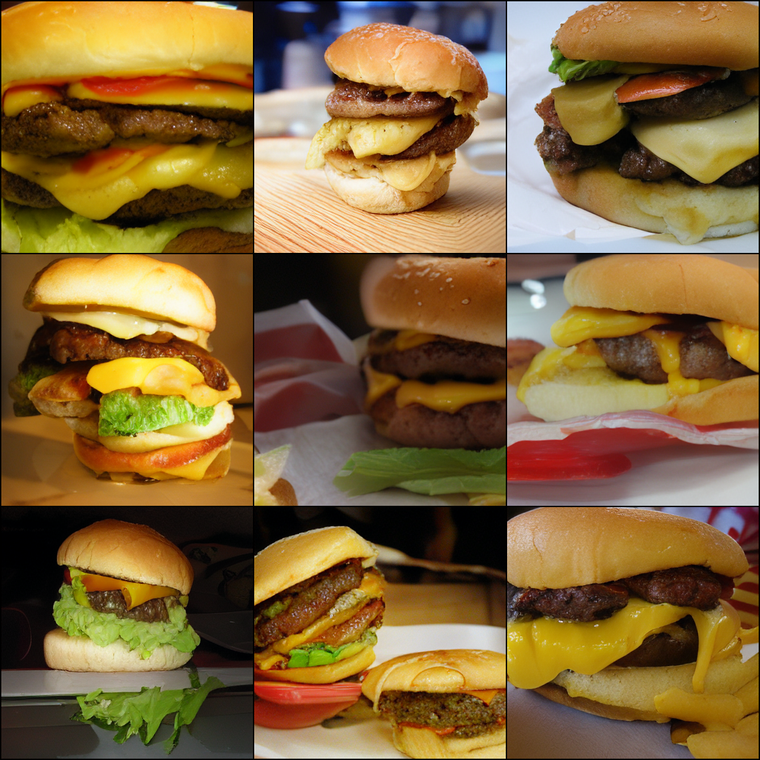
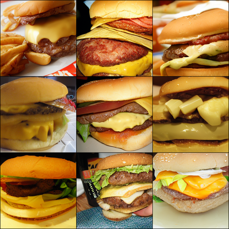
Figure 3 presents a qualitative comparison of image samples before and after CCA fine-tuning. The results clearly demonstrate that CCA can vastly improve image fidelity, as well as class-image alignment of guidance-free samples.
Table 2 compares our best-performing models with several state-of-the-art visual generative models. With the help of CCA, we achieve a record-breaking FID score of 2.54 and an IS score of 276.8 for guidance-free samples of AR visual models. Although these numbers still somewhat lag behind CFG-enhanced performance, they demonstrate the significant potential of alignment algorithms to enhance visual generation and indicate the future possibility of replacing guided sampling.
5.2 Controllable Trade-Offs between Diversity and Fidelity
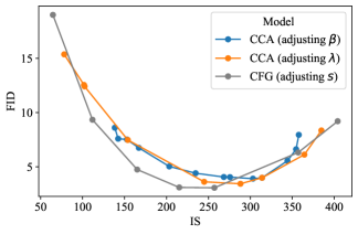
A distinctive feature of CFG is its ability to balance diversity and fidelity by adjusting the guidance scale. It is reasonable to expect that CCA can achieve a similar trade-off since it essentially targets the same sampling distribution as CFG.
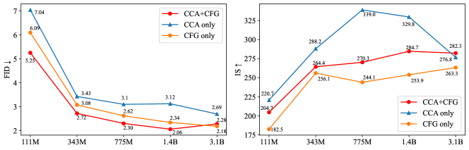
Figure 4 confirms this expectation: by adjusting the parameter for fine-tuning, CCA can achieve similar FID-IS trade-offs to CFG. The key difference is that CCA enhances guidance-free models through training, while CFG mainly improves the sampling process.
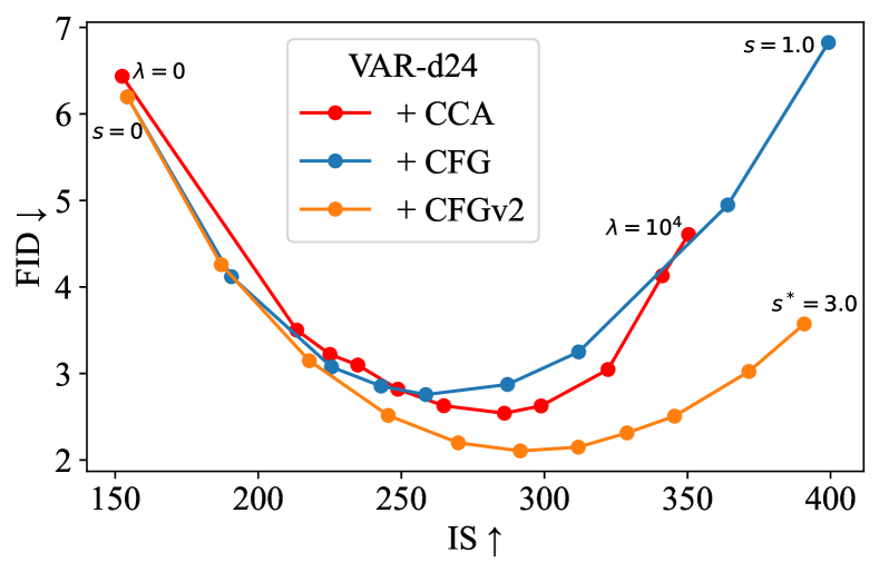
It is worth noting that VAR employs a slightly different guidance technique from standard CFG, which we refer to as CFGv2. CFGv2 involves linearly increasing the guidance scale during sampling, which was first proposed by Chang et al. (2023) and found beneficial for certain models. The FID-IS curve of CCA more closely resembles that of standard CFG. Additionally, the hyperparameter also affects CCA performance. Although our algorithm derivation shows that is directly related to the CFG scale , we empirically find adjusting is less effective and less predictable compared with adjusting . In practice, we typically fix and adjust . We ablate in Appendix C.
5.3 Can LLM Alignment Algorithms also Enhance Visual AR?
| Model | FID | IS | sFID | Precision | Recall |
|---|---|---|---|---|---|
| LlamaGen-L | 19.00 | 64.7 | 8.78 | 0.61 | 0.67 |
| DPO | 61.69 | 30.8 | 44.98 | 0.36 | 0.40 |
| Unlearn | 12.22 | 111.6 | 7.99 | 0.66 | 0.64 |
| CCA | 3.43 | 288.2 | 7.44 | 0.81 | 0.52 |
| Model | FID | IS | sFID | Precision | Recall |
|---|---|---|---|---|---|
| VAR-d24 | 6.20 | 154.3 | 8.50 | 0.74 | 0.62 |
| DPO | 7.53 | 232.6 | 19.10 | 0.85 | 0.34 |
| Unlearn | 5.55 | 165.9 | 8.41 | 0.75 | 0.61 |
| CCA | 2.63 | 298.8 | 7.63 | 0.84 | 0.55 |
Intuitively, existing preference-based LLM alignment algorithms such as DPO and Unlearning (Welleck et al., 2019) should also offer improvement for AR visual models given their similarity to CCA. However, Table 3 shows that naive applications of these methods fail significantly.
DPO.
As is described in Eq. 5, one can treat negative image-condition pairs as dispreferred data and positive ones as preferred data to apply the DPO loss. We ablate and report the best performance in Table 3. Results indicate that DPO fails to enhance pretrained models, even causing performance collapse for LlamaGen-L. By inspecting training logs, we find that the likelihood of the positive data continuously decreases during fine-tuning, which may explain the collapse. This phenomenon is a well-observed problem of DPO (Chen et al., 2024a; Pal et al., 2024), stemming from its focus on optimizing only the relative likelihood between preferred and dispreferred data, rather than controlling likelihood for positive and negative image-condition pairs separately. We refer interested readers to Chen et al. (2024a) for a detailed discussion.
Unlearning.
Also known as unlikelihood training, this method maximizes through standard maximum likelihood training on positive data, while minimizing to unlearn negative data. A training parameter controls the weight of the unlearning loss. We find that with small , Unlearning provides some benefit, but it is far less effective than CCA. This suggests the necessity of including a frozen reference model.
5.4 Integration of CCA and CFG
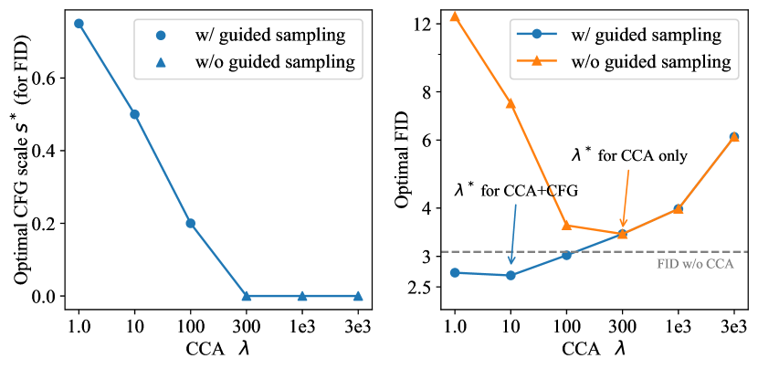
If extra sampling costs and design inconsistencies of CFG are not concerns, could CCA still be helpful? A takeaway conclusion is yes: CCA+CFG generally outperforms CFG (Figure 6), but it requires distinct hyperparameter choices compared with CCA-only training.
Implementation.
After pretraining the unconditional AR visual model by randomly dropping conditions, CFG requires us to also fine-tune the unconditional model during alignment. To achieve this, we follow previous approaches by also randomly replacing data conditions with [MASK] tokens at a probability of 10%. These unconditional samples are treated as positive data during CCA training.
Comparison of CCA-only and CCA+CFG.
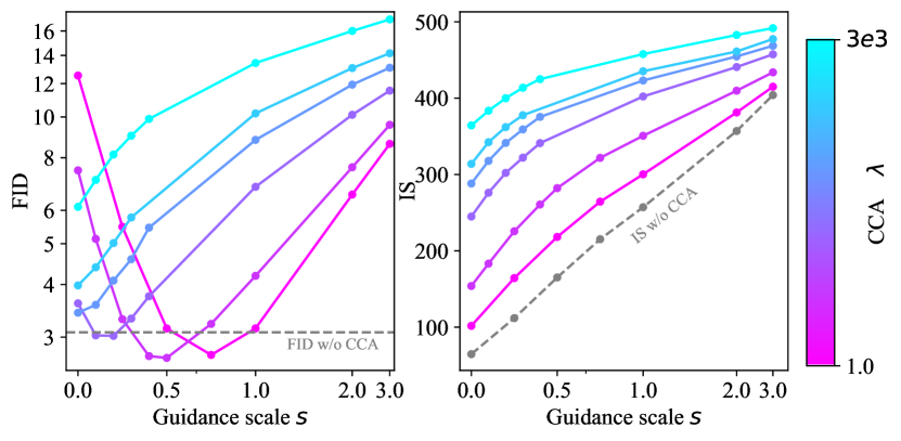
They require different hyperparameters. As shown in Figure 5, a larger is typically needed for optimal FID scores in guidance-free generation. For models optimized for guidance-free sampling, adding CFG guidance does not further reduce the FID score. However, with a smaller , CCA+CFG could outperform the CFG method.
6 Related Works
Visual generative models.
Generative adversarial networks (GANs) (Goodfellow et al., 2014; Brock et al., 2018; Karras et al., 2019; Kang et al., 2023) and diffusion models (Ho et al., 2020; Song & Ermon, 2019; Song et al., 2020; Dhariwal & Nichol, 2021; Kingma & Gao, 2024) are representative modeling methods for visual content generation, widely recognized for their ability to produce realistic and artistic images (Sauer et al., 2022; Ho et al., 2022; Ramesh et al., 2022; Podell et al., 2023). However, because these methods are designed for continuous data like images, they struggle to effectively model discrete data such as text, limiting the development of unified multimodal models for both vision and language. Recent approaches seek to address this by integrating diffusion models with language models (Team, 2024; Li et al., 2024; Zhou et al., 2024). Another line of works (Chang et al., 2022; 2023; Yu et al., 2023; Xie et al., 2024; Ramesh et al., 2021; Yu et al., 2022) explores discretizing images (Van Den Oord et al., 2017; Esser et al., 2021) and directly applying language models such as BERT-style (Devlin et al., 2018) masked-prediction models and GPT-style (Radford et al., 2018) autoregressive models for image generation.
Language model alignment.
Different from visual generative models which generally enhance sample quality through sampling-based methods (Dhariwal & Nichol, 2021; Ho & Salimans, 2022; Zhao et al., 2022; Lu et al., 2023), LLMs primarily employ training-based alignment techniques to improve instruction-following abilities (Touvron et al., 2023b; OpenAI, 2023). Reinforcement Learning (RL) is well-suited for aligning LLMs with human feedback (Schulman et al., 2017; Ouyang et al., 2022). However, this method requires learning a reward model before optimizing LLMs, leading to an indirect two-stage optimization process. Recent developments in alignment techniques (Rafailov et al., 2023; Cai et al., 2023; Azar et al., 2024; Ethayarajh et al., 2024; Chen et al., 2024a; Ji et al., 2024) have streamlined this process. They enable direct alignment of LMs through a singular loss. Among all LLM alignment algorithms, our method is perhaps most similar to NCA (Chen et al., 2024a). Both NCA and CCA are theoretically grounded in the NCE framework (Gutmann & Hyvärinen, 2012). Their differences are mainly empirical regarding loss implementations, particularly in how to estimate expectations under the product of two marginal distributions.
Visual alignment.
Motivated by the success of alignment techniques in LLMs, several studies have also investigated aligning visual generative models with human preferences using RL (Black et al., 2023a; Xu et al., 2024) or DPO (Black et al., 2023b; Wallace et al., 2023). For diffusion models, the application is not straightforward and must rely on some theoretical approximations, as diffusion models do not allow direct likelihood calculation, which is required by most LLM alignment algorithms (Chen et al., 2024b). Moreover, previous attempts at visual alignment have primarily focused on enhancing the aesthetic quality of generated images and necessitate a different dataset from the pretrained one. Our work distinguishes itself from prior research by having a fundamentally different optimization objective (replacing CFG) and does not rely on any additional data input.
7 Conclusion
In this paper, we propose Condition Contrastive Alignment (CCA) as a fine-tuning algorithm for AR visual generation models. CCA can significantly enhance the guidance-free sample quality of pretrained models without any modification of the sampling process. This paves the way for further development in multimodal generative models and cuts the cost of AR visual generation by half in comparison to CFG. Our research also highlights the strong theoretical connection between language-targeted alignment and visual-targeted guidance methods, facilitating future research of unifying visual modeling and language modeling.
Acknowledgments
We thank Fan Bao, Kai Jiang, Xiang Li, and Min Zhao for providing valuable suggestions. We thank Keyu Tian and Kaiwen Zheng for the discussion.
References
- Azar et al. (2024) Mohammad Gheshlaghi Azar, Zhaohan Daniel Guo, Bilal Piot, Remi Munos, Mark Rowland, Michal Valko, and Daniele Calandriello. A general theoretical paradigm to understand learning from human preferences. In International Conference on Artificial Intelligence and Statistics, pp. 4447–4455. PMLR, 2024.
- Bao et al. (2023) Fan Bao, Shen Nie, Kaiwen Xue, Yue Cao, Chongxuan Li, Hang Su, and Jun Zhu. All are worth words: A vit backbone for diffusion models. In Proceedings of the IEEE/CVF conference on computer vision and pattern recognition, pp. 22669–22679, 2023.
- Black et al. (2023a) Kevin Black, Michael Janner, Yilun Du, Ilya Kostrikov, and Sergey Levine. Training diffusion models with reinforcement learning. arXiv preprint arXiv:2305.13301, 2023a.
- Black et al. (2023b) Kevin Black, Michael Janner, Yilun Du, Ilya Kostrikov, and Sergey Levine. Training diffusion models with reinforcement learning. arXiv preprint arXiv:2305.13301, 2023b.
- Bradley & Terry (1952) Ralph Allan Bradley and Milton E Terry. Rank analysis of incomplete block designs: I. the method of paired comparisons. Biometrika, 39(3/4):324–345, 1952.
- Brock et al. (2018) Andrew Brock, Jeff Donahue, and Karen Simonyan. Large scale gan training for high fidelity natural image synthesis. arXiv preprint arXiv:1809.11096, 2018.
- Cai et al. (2023) Tianchi Cai, Xierui Song, Jiyan Jiang, Fei Teng, Jinjie Gu, and Guannan Zhang. Ulma: Unified language model alignment with demonstration and point-wise human preference. arXiv preprint arXiv:2312.02554, 2023.
- Chang et al. (2022) Huiwen Chang, Han Zhang, Lu Jiang, Ce Liu, and William T Freeman. Maskgit: Masked generative image transformer. In Proceedings of the IEEE/CVF Conference on Computer Vision and Pattern Recognition, pp. 11315–11325, 2022.
- Chang et al. (2023) Huiwen Chang, Han Zhang, Jarred Barber, AJ Maschinot, Jose Lezama, Lu Jiang, Ming-Hsuan Yang, Kevin Murphy, William T Freeman, Michael Rubinstein, et al. Muse: Text-to-image generation via masked generative transformers. arXiv preprint arXiv:2301.00704, 2023.
- Chen et al. (2024a) Huayu Chen, Guande He, Hang Su, and Jun Zhu. Noise contrastive alignment of language models with explicit rewards. Advances in neural information processing systems, 2024a.
- Chen et al. (2024b) Huayu Chen, Kaiwen Zheng, Hang Su, and Jun Zhu. Aligning diffusion behaviors with q-functions for efficient continuous control. Advances in neural information processing systems, 2024b.
- Devlin et al. (2018) Jacob Devlin, Ming-Wei Chang, Kenton Lee, and Kristina Toutanova. Bert: Pre-training of deep bidirectional transformers for language understanding. arXiv preprint arXiv:1810.04805, 2018.
- Dhariwal & Nichol (2021) Prafulla Dhariwal and Alexander Nichol. Diffusion models beat gans on image synthesis. Advances in neural information processing systems, 34:8780–8794, 2021.
- Esser et al. (2021) Patrick Esser, Robin Rombach, and Bjorn Ommer. Taming transformers for high-resolution image synthesis. In Proceedings of the IEEE/CVF conference on computer vision and pattern recognition, pp. 12873–12883, 2021.
- Ethayarajh et al. (2024) Kawin Ethayarajh, Winnie Xu, Niklas Muennighoff, Dan Jurafsky, and Douwe Kiela. Kto: Model alignment as prospect theoretic optimization. arXiv preprint arXiv:2402.01306, 2024.
- Gao et al. (2023) Shanghua Gao, Pan Zhou, Ming-Ming Cheng, and Shuicheng Yan. Masked diffusion transformer is a strong image synthesizer. In Proceedings of the IEEE/CVF International Conference on Computer Vision, pp. 23164–23173, 2023.
- Goodfellow et al. (2014) Ian Goodfellow, Jean Pouget-Abadie, Mehdi Mirza, Bing Xu, David Warde-Farley, Sherjil Ozair, Aaron Courville, and Yoshua Bengio. Generative adversarial nets. Advances in neural information processing systems, 27, 2014.
- Gutmann & Hyvärinen (2012) Michael U Gutmann and Aapo Hyvärinen. Noise-contrastive estimation of unnormalized statistical models, with applications to natural image statistics. Journal of machine learning research, 13(2), 2012.
- Heusel et al. (2017) Martin Heusel, Hubert Ramsauer, Thomas Unterthiner, Bernhard Nessler, and Sepp Hochreiter. Gans trained by a two time-scale update rule converge to a local nash equilibrium. Advances in neural information processing systems, 30, 2017.
- Ho & Salimans (2022) Jonathan Ho and Tim Salimans. Classifier-free diffusion guidance. arXiv preprint arXiv:2207.12598, 2022.
- Ho et al. (2020) Jonathan Ho, Ajay Jain, and Pieter Abbeel. Denoising diffusion probabilistic models. Advances in neural information processing systems, 33:6840–6851, 2020.
- Ho et al. (2022) Jonathan Ho, Chitwan Saharia, William Chan, David J Fleet, Mohammad Norouzi, and Tim Salimans. Cascaded diffusion models for high fidelity image generation. The Journal of Machine Learning Research, 23(1):2249–2281, 2022.
- Ji et al. (2024) Haozhe Ji, Cheng Lu, Yilin Niu, Pei Ke, Hongning Wang, Jun Zhu, Jie Tang, and Minlie Huang. Towards efficient and exact optimization of language model alignment. arXiv preprint arXiv:2402.00856, 2024.
- Kang et al. (2023) Minguk Kang, Jun-Yan Zhu, Richard Zhang, Jaesik Park, Eli Shechtman, Sylvain Paris, and Taesung Park. Scaling up gans for text-to-image synthesis. In Proceedings of the IEEE/CVF Conference on Computer Vision and Pattern Recognition, pp. 10124–10134, 2023.
- Karras et al. (2019) Tero Karras, Samuli Laine, and Timo Aila. A style-based generator architecture for generative adversarial networks. In Proceedings of the IEEE/CVF conference on computer vision and pattern recognition, pp. 4401–4410, 2019.
- Kingma & Gao (2024) Diederik Kingma and Ruiqi Gao. Understanding diffusion objectives as the elbo with simple data augmentation. Advances in Neural Information Processing Systems, 36, 2024.
- Lee et al. (2022) Doyup Lee, Chiheon Kim, Saehoon Kim, Minsu Cho, and Wook-Shin Han. Autoregressive image generation using residual quantization. In Proceedings of the IEEE/CVF Conference on Computer Vision and Pattern Recognition, pp. 11523–11532, 2022.
- Li et al. (2023) Tianhong Li, Huiwen Chang, Shlok Mishra, Han Zhang, Dina Katabi, and Dilip Krishnan. Mage: Masked generative encoder to unify representation learning and image synthesis. In Proceedings of the IEEE/CVF Conference on Computer Vision and Pattern Recognition, pp. 2142–2152, 2023.
- Li et al. (2024) Tianhong Li, Yonglong Tian, He Li, Mingyang Deng, and Kaiming He. Autoregressive image generation without vector quantization. arXiv preprint arXiv:2406.11838, 2024.
- Lu et al. (2023) Cheng Lu, Huayu Chen, Jianfei Chen, Hang Su, Chongxuan Li, and Jun Zhu. Contrastive energy prediction for exact energy-guided diffusion sampling in offline reinforcement learning. In International Conference on Machine Learning, pp. 22825–22855. PMLR, 2023.
- OpenAI (2023) OpenAI. Gpt-4 technical report. arXiv preprint arXiv:2303.08774, 2023.
- Ouyang et al. (2022) Long Ouyang, Jeffrey Wu, Xu Jiang, Diogo Almeida, Carroll Wainwright, Pamela Mishkin, Chong Zhang, Sandhini Agarwal, Katarina Slama, Alex Ray, et al. Training language models to follow instructions with human feedback. Advances in neural information processing systems, 35:27730–27744, 2022.
- Pal et al. (2024) Arka Pal, Deep Karkhanis, Samuel Dooley, Manley Roberts, Siddartha Naidu, and Colin White. Smaug: Fixing failure modes of preference optimisation with dpo-positive. arXiv preprint arXiv:2402.13228, 2024.
- Peebles & Xie (2023) William Peebles and Saining Xie. Scalable diffusion models with transformers. In Proceedings of the IEEE/CVF International Conference on Computer Vision, pp. 4195–4205, 2023.
- Podell et al. (2023) Dustin Podell, Zion English, Kyle Lacey, Andreas Blattmann, Tim Dockhorn, Jonas Müller, Joe Penna, and Robin Rombach. Sdxl: Improving latent diffusion models for high-resolution image synthesis. arXiv preprint arXiv:2307.01952, 2023.
- Radford et al. (2018) Alec Radford, Karthik Narasimhan, Tim Salimans, Ilya Sutskever, et al. Improving language understanding by generative pre-training. article, 2018.
- Rafailov et al. (2023) Rafael Rafailov, Archit Sharma, Eric Mitchell, Christopher D Manning, Stefano Ermon, and Chelsea Finn. Direct preference optimization: Your language model is secretly a reward model. In Thirty-seventh Conference on Neural Information Processing Systems, 2023.
- Ramesh et al. (2021) Aditya Ramesh, Mikhail Pavlov, Gabriel Goh, Scott Gray, Chelsea Voss, Alec Radford, Mark Chen, and Ilya Sutskever. Zero-shot text-to-image generation. In International Conference on Machine Learning, pp. 8821–8831. PMLR, 2021.
- Ramesh et al. (2022) Aditya Ramesh, Prafulla Dhariwal, Alex Nichol, Casey Chu, and Mark Chen. Hierarchical text-conditional image generation with clip latents. arXiv preprint arXiv:2204.06125, 1(2):3, 2022.
- Rombach et al. (2022) Robin Rombach, Andreas Blattmann, Dominik Lorenz, Patrick Esser, and Björn Ommer. High-resolution image synthesis with latent diffusion models. In Proceedings of the IEEE/CVF conference on computer vision and pattern recognition, pp. 10684–10695, 2022.
- Salimans et al. (2016) Tim Salimans, Ian Goodfellow, Wojciech Zaremba, Vicki Cheung, Alec Radford, and Xi Chen. Improved techniques for training gans. Advances in neural information processing systems, 29, 2016.
- Sauer et al. (2022) Axel Sauer, Katja Schwarz, and Andreas Geiger. Stylegan-xl: Scaling stylegan to large diverse datasets. In ACM SIGGRAPH 2022 conference proceedings, pp. 1–10, 2022.
- Schulman et al. (2017) John Schulman, Filip Wolski, Prafulla Dhariwal, Alec Radford, and Oleg Klimov. Proximal policy optimization algorithms. arXiv preprint arXiv:1707.06347, 2017.
- Schulman et al. (2022) John Schulman, Barret Zoph, Christina Kim, Jacob Hilton, Jacob Menick, Jiayi Weng, Juan Felipe Ceron Uribe, Liam Fedus, Luke Metz, Michael Pokorny, et al. Chatgpt: Optimizing language models for dialogue. OpenAI blog, 2022.
- Song et al. (2020) Jiaming Song, Chenlin Meng, and Stefano Ermon. Denoising diffusion implicit models. arXiv preprint arXiv:2010.02502, 2020.
- Song & Ermon (2019) Yang Song and Stefano Ermon. Generative modeling by estimating gradients of the data distribution. Advances in neural information processing systems, 32, 2019.
- Sun et al. (2024) Peize Sun, Yi Jiang, Shoufa Chen, Shilong Zhang, Bingyue Peng, Ping Luo, and Zehuan Yuan. Autoregressive model beats diffusion: Llama for scalable image generation. arXiv preprint arXiv:2406.06525, 2024.
- Team (2024) Chameleon Team. Chameleon: Mixed-modal early-fusion foundation models. arXiv preprint arXiv:2405.09818, 2024.
- Tian et al. (2024) Keyu Tian, Yi Jiang, Zehuan Yuan, Bingyue Peng, and Liwei Wang. Visual autoregressive modeling: Scalable image generation via next-scale prediction. arXiv preprint arXiv:2404.02905, 2024.
- Touvron et al. (2023a) Hugo Touvron, Thibaut Lavril, Gautier Izacard, Xavier Martinet, Marie-Anne Lachaux, Timothée Lacroix, Baptiste Rozière, Naman Goyal, Eric Hambro, Faisal Azhar, et al. Llama: Open and efficient foundation language models. arXiv preprint arXiv:2302.13971, 2023a.
- Touvron et al. (2023b) Hugo Touvron, Louis Martin, Kevin Stone, Peter Albert, Amjad Almahairi, Yasmine Babaei, Nikolay Bashlykov, Soumya Batra, Prajjwal Bhargava, Shruti Bhosale, et al. Llama 2: Open foundation and fine-tuned chat models. arXiv preprint arXiv:2307.09288, 2023b.
- Van Den Oord et al. (2017) Aaron Van Den Oord, Oriol Vinyals, et al. Neural discrete representation learning. Advances in neural information processing systems, 30, 2017.
- Wallace et al. (2023) Bram Wallace, Meihua Dang, Rafael Rafailov, Linqi Zhou, Aaron Lou, Senthil Purushwalkam, Stefano Ermon, Caiming Xiong, Shafiq Joty, and Nikhil Naik. Diffusion model alignment using direct preference optimization. arXiv preprint arXiv:2311.12908, 2023.
- Welleck et al. (2019) Sean Welleck, Ilia Kulikov, Stephen Roller, Emily Dinan, Kyunghyun Cho, and Jason Weston. Neural text generation with unlikelihood training. arXiv preprint arXiv:1908.04319, 2019.
- Xie et al. (2024) Jinheng Xie, Weijia Mao, Zechen Bai, David Junhao Zhang, Weihao Wang, Kevin Qinghong Lin, Yuchao Gu, Zhijie Chen, Zhenheng Yang, and Mike Zheng Shou. Show-o: One single transformer to unify multimodal understanding and generation. arXiv preprint arXiv:2408.12528, 2024.
- Xu et al. (2024) Jiazheng Xu, Xiao Liu, Yuchen Wu, Yuxuan Tong, Qinkai Li, Ming Ding, Jie Tang, and Yuxiao Dong. Imagereward: Learning and evaluating human preferences for text-to-image generation. Advances in Neural Information Processing Systems, 36, 2024.
- Yu et al. (2021) Jiahui Yu, Xin Li, Jing Yu Koh, Han Zhang, Ruoming Pang, James Qin, Alexander Ku, Yuanzhong Xu, Jason Baldridge, and Yonghui Wu. Vector-quantized image modeling with improved vqgan. arXiv preprint arXiv:2110.04627, 2021.
- Yu et al. (2022) Jiahui Yu, Yuanzhong Xu, Jing Yu Koh, Thang Luong, Gunjan Baid, Zirui Wang, Vijay Vasudevan, Alexander Ku, Yinfei Yang, Burcu Karagol Ayan, et al. Scaling autoregressive models for content-rich text-to-image generation. arXiv preprint arXiv:2206.10789, 2(3):5, 2022.
- Yu et al. (2023) Lijun Yu, José Lezama, Nitesh B Gundavarapu, Luca Versari, Kihyuk Sohn, David Minnen, Yong Cheng, Agrim Gupta, Xiuye Gu, Alexander G Hauptmann, et al. Language model beats diffusion–tokenizer is key to visual generation. arXiv preprint arXiv:2310.05737, 2023.
- Zhao et al. (2022) Min Zhao, Fan Bao, Chongxuan Li, and Jun Zhu. Egsde: Unpaired image-to-image translation via energy-guided stochastic differential equations. Advances in Neural Information Processing Systems, 35:3609–3623, 2022.
- Zhou et al. (2024) Chunting Zhou, Lili Yu, Arun Babu, Kushal Tirumala, Michihiro Yasunaga, Leonid Shamis, Jacob Kahn, Xuezhe Ma, Luke Zettlemoyer, and Omer Levy. Transfusion: Predict the next token and diffuse images with one multi-modal model. arXiv preprint arXiv:2408.11039, 2024.

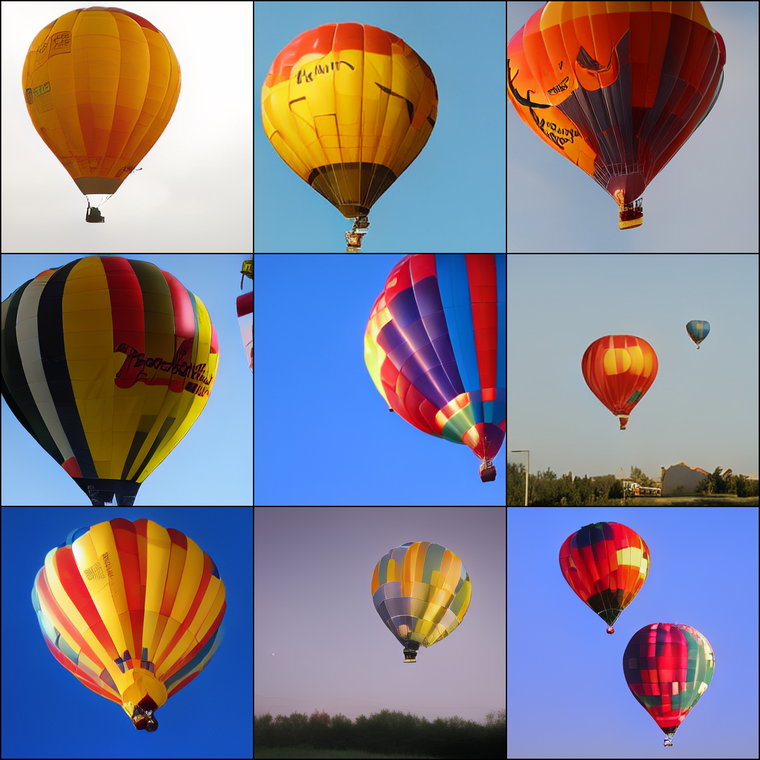
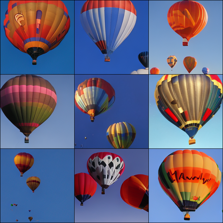
w/o Guidance
+CCA (w/o Guidance)
w/ CFG Guidance
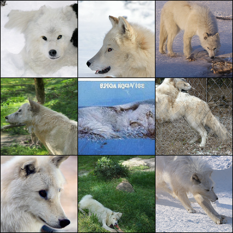
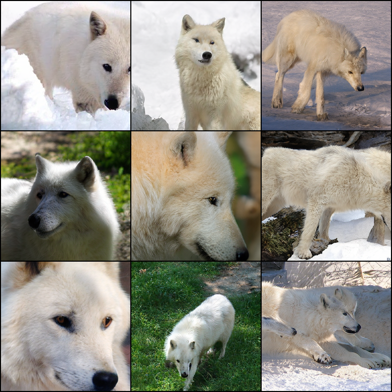
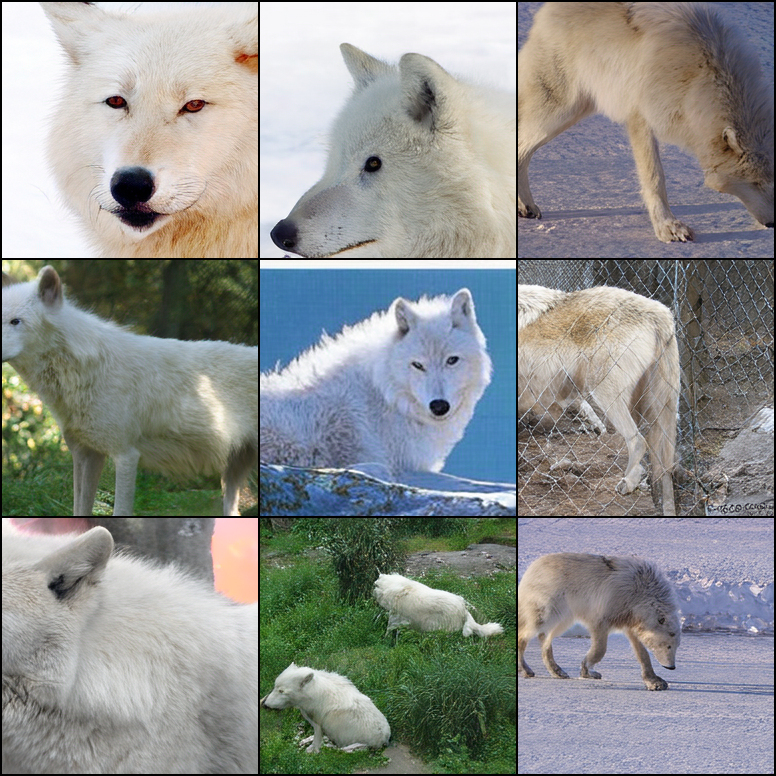
w/o Guidance
+CCA (w/o Guidance)
w/ CFG Guidance
Appendix A Theoretical Proofs
In this section, we provide the proof of Theorem 3.1.
Theorem A.1 (Noise Contrastive Estimation ).
Let be a parameterized model which takes in an image-condition pair and outputs a scalar value . Consider the loss function:
| (13) |
Given unlimited model expressivity for , the optimal solution for minimizing satisfies
| (14) |
Proof.
First, we construct two binary (Bernoulli) distributions:
Then we rewrite as
Here represents the cross-entropy between distributions and . is the entropy of , which can be regarded as a constant number with respect to parameter . Due to the theoretical properties of KL-divergence, we have
constantly hold. The equality holds if and only if , such that
∎
Appendix B Theoretical Analyses of the Normalizing Constant
We omit a normalizing constant in Eq. 7 for brevity when deriving CCA. Strictly speaking, the target sampling distribution should be:
such that
The normalizing constant ensures that is properly normalized, i.e., . We have .
To mitigate the additional effects introduced by , in our practical algorithm, we introduce a new training parameter to bias the optimal solution for Noise Contrastive Estimation. Below, we present a result that is stronger than Theorem 3.1.
Theorem B.1.
Let be a scalar function conditioned only on . Consider the loss function:
| (15) |
Given unlimited model expressivity for , the optimal solution for minimizing satisfies
| (16) |
Proof.
If let , we could guarantee the convergence of to . However, in practice estimating could be intricately difficult, so we formalize as a training parameter, resulting in our practical algorithm in Eq. 12.
Appendix C Additional Experimental Results
We illustrate the effect of training parameter on the FID-IS trade-off in Figure 9. Overall, affects the fidelity-diversity trade-off similar to CCA and the CFG method.
Appendix D Training Hyperparameters
Table 4 reports hyperparameters for chosen models in Figure 1 and Figure 6. Other unmentioned design choices and hyperparameters are consistent with the default setting for LlamaGen https://github.com/FoundationVision/LlamaGen and VAR https://github.com/FoundationVision/VAR repo. All models are fine-tuned for 1 epoch on the ImageNet dataset. We use a mix of NVIDIA-H100, NVIDIA A100, and NVIDIA A40 GPU cards for training.
| Type | LlamaGen | VAR | |||||||
|---|---|---|---|---|---|---|---|---|---|
| Model | B | L | XL | XXL | 3B | d16 | d20 | d24 | d30 |
| Size | 111M | 343M | 775M | 1.4B | 3.1B | 310M | 600M | 1.0B | 2.0B |
| CCA | 0.02 | 0.02 | 0.02 | 0.02 | 0.02 | 0.02 | 0.02 | 0.02 | 0.02 |
| CCA | 1000 | 300 | 1000 | 1000 | 500 | 50 | 50 | 100 | 1000 |
| CCA+CFG | 0.1 | 0.02 | 0.1 | 0.1 | 0.1 | - | - | - | - |
| CCA+CFG | 1 | 1 | 1 | 1 | 1 | - | - | - | - |
| Learning rate | 1e-5 | 1e-5 | 1e-5 | 1e-5 | 1e-5 | 2e-5 | 2e-5 | 2e-5 | 2e-5 |
| Dropout? | Yes | Yes | Yes | Yes | Yes | None | Yes | Yes | Yes |
| Batch size | 256 | 256 | 256 | 256 | 256 | 256 | 256 | 256 | 256 |