Toward Causal-Aware RL:
State-Wise Action-Refined Temporal Difference

Hao Sun
[email protected] &Taiyi Wang
[email protected]

Abstract

Although it is well known that exploration plays a key role in Reinforcement Learning (RL), prevailing exploration strategies for continuous control tasks in RL are mainly based on naive isotropic Gaussian noise regardless of the causality relationship between action space and the task and consider all dimensions of actions equally important. In this work, we propose to conduct interventions on the primal action space to discover the causal relationship between the action space and the task reward. We propose the method of State-Wise Action Refined (SWAR), which addresses the issue of action space redundancy and promote causality discovery in RL. We formulate causality discovery in RL tasks as a state-dependent action space selection problem and propose two practical algorithms as solutions. The first approach, TD-SWAR, detects task-related actions during temporal difference learning, while the second approach, Dyn-SWAR, reveals important actions through dynamic model prediction. Empirically, both methods provide approaches to understand the decisions made by RL agents and improve learning efficiency in action-redundant tasks.

1 Introduction

Although model-free RL has achieved great success in various challenging tasks and outperforms experts in most cases [21, 26, 17, 33, 4], the design of action space always requires elaboration. For example, in the game StarCraftII, hundreds of units can be selected and controlled to perform various actions. To tackle the difficulty in exploration caused by the extremely large action and state space, hierarchical action space design and imitation learning are used [27, 33] to reduce the exploration space. Both of those approaches require expert knowledge of the task. On the other hand, even in the context of imitation learning where expert data is assumed to be accessible, causal confusion will still hinder the performance of an agent [8]. Those defects motivate us to explore the causality-awareness of an agent that permits an agent to discover the causal relationship for the environment and select useful dimensions of action space during policy learning in pursuance of improved learning efficiency. Another motivating example is the in-hand manipulation tasks [2]: robotics equipped with touch sensors outperforms the policies learned without sensors by a clear margin in hand-in manipulation tasks [20], showing the importance of causality discovery between actions and feedbacks in RL. A similar example can be found in human learning: knowing nothing about how to control the finger joints flexibly may not hinder a baby learns to walk, and a baby has not learned how to walk can still learn to use forks and spoons skillfully, inspiring us to believe that the challenge for exploration can be greatly eased after the causality between action space and the given task is learned.

In this work, the recent advance of instance-wise feature selection technique [37] is improved to be more suitable in large-scale state-wise action selection tasks and adapted to the time-series causal discovery setting to select state-conditioned action space in RL with redundant action space. With the proposed method, the agent learns to perform intervention, discover the true structural causal model (SCM) and select task-related actions for a given task, remarkably reduces the burden of exploration and obtains on-par learning efficiency as well as asymptotic performance compared with agents trained in the oracle settings where the action spaces are pruned according to given tasks manually.

2 Preliminary

Refer to caption — Figure 1: Block diagram of INVASE in temporal difference learning. States and actions sampled from replay buffer are fed into the selector network that predicts the selection probabilities of different dimensions of actions. A selection mask is then generated according to such a selection probability vector. The critic network and the baseline network are trained to minimize temporal difference error with states and the selected dimension of actions and primal action respectively. The difference of TD-Error is used to conduct a policy gradient to update the selector network.

Markov Decision Processes

RL tasks can be formally defined as Markov Decision Processes (MDPs), where an agent interacts with the environment and learns to make decision at every timestep. Formally, we consider the deterministic MDP with a fixed horizon $H\in\mathbb{N}^{+}$ denoted by a tuple $(\mathcal{S},\mathcal{A},H,r,\gamma,\mathcal{T},\rho_{0})$ , where $\mathcal{S}$ and $\mathcal{A}$ are the $|\mathcal{S}|$ -dimensional state and $|\mathcal{A}|$ -dimensional action space; $r:\mathcal{S}\times\mathcal{A}\mapsto\mathbb{R}$ denotes the reward function; $\gamma\in(0,1]$ is the discount factor indicating importance of present returns compared with long-term returns; $\mathcal{T}:\mathcal{S}\times\mathcal{A}\mapsto\mathcal{S}$ denotes the transition dynamics; $\rho_{0}$ is the initial state distribution.

We use $\Pi$ to represent the stationary deterministic policy class, i.e., $\Pi=\{\pi:\mathcal{S}\mapsto\mathcal{A}\}$ . The learning objective of an RL algorithm is to find $\pi^{*}\in\Pi$ as the solution of the following optimization problem: $\max_{\pi\in\Pi}\mathbb{E}_{\tau\sim\rho_{0},\pi,\mathcal{T}}[\sum_{t=1}^{H}\gamma^{t}r_{t}]$ where the expectation is taken over the trajectory $\tau=(s_{1},a_{1},r_{1},\dots,s_{H},a_{H},r_{H})$ generated by policy $\pi$ under the environment $\mathcal{T}$ , starting from $s_{0}\sim\rho_{0}$ .

INVASE

INVASE is proposed by [37] to perform instance-wise feature selection to reduce overfitting in predictive models. The learning objective is to minimize the KL-Divergence of the full-conditional distribution and the minimal-selected-features-only conditional distribution of the outcome, i.e., $\min_{F}\mathcal{L}$ , with

\begin{array}[]{ll}\mathcal{L}=\mathcal{D}_{KL}(p(Y|X=x)||p(Y|X^{(F(x))}=x^{(F(x)})))+\lambda|F(x)|_{0}.\end{array}

(1)

where $F:\mathcal{X}\to\{0,1\}^{d}$ is a feature selection function and $|F(x)|_{0}$ denotes the cardinality ( $l_{0}$ norm) of selected features, i.e., the number of $1$ ’s in $F(x)$ . ¹¹1To avoid confusion between state notion $s\in\mathcal{S}$ and the selector notion $S$ used in [37], $F$ is used in this work to represent the selector (i.e., mask generator). $d$ is the dimension of input features. $x^{(F(x))}=F(x)\odot x$ denotes the element-wise product of $x$ and generated mask $m=F(x)$ . Ideally, the optimal selection function $F$ should be able to minimize the two terms in Equation (1) simultaneously.

INVASE applies the Actor-Critic framework in the optimization of $F$ through sampling, where $f_{\theta}(\cdot|x)$ , parameterized by a neural network $\theta$ ²²2In this work, subscripts $\phi,\psi,\theta,w$ are used to denote the parameter of neural networks., is used as a stochastic actor. Two predictive networks $C_{\phi}(\cdot),B_{\psi}(\cdot)$ are considered as the critic and the baseline network used for variance reduction [35] and trained with the Cross-Entropy loss to produce return signal $\mathcal{L}$ , based on which $f_{\theta}(\cdot|x)$ can be optimized through policy gradient:

\mathbb{E}_{(x,y)\sim p}[\mathbb{E}_{m\sim f_{\theta}(\cdot|x)}[\mathcal{L}\nabla_{\theta}\log f_{\theta}(\cdot|x)]].

(2)

Finally, $F(x)=(F_{1}(x),...,F_{d}(x))$ can be get by sampling from $f(\cdot|x)=(f_{1}(x),...,f_{d}(x))$ , with

F_{i}(x)=\begin{cases}1,\quad\mathbf{w.p.}\quad f_{i}(\cdot|x).\\ 0,\quad\mathbf{w.p.}\quad 1-f_{i}(\cdot|x).\end{cases}

(3)

3 Proposed Method

The objective of this work is to carry out state-wise action selection in RL through intervention, and thereby enhance the learning efficiency with a pruned task-related action space after finding the correct causal model. Section 3.1 starts with the formalization of the action space refinery objective in RL tasks under the framework of causal discovery. Section 3.2 introduces SWAR, which improves the scalability of INVASE in high dimensional variable selection tasks. We integrate SWAR with deterministic policy gradient methods [25] in Section 3.3 to perform state-wise action space pruning, resulting in two practical causality-aware RL algorithms.

3.1 Temporal Difference Objective with Structural Causal Models

In modern RL algorithms, the most general approach is based on the Actor-Critic framework [15], where the critic $Q_{w}(s,a)$ approximates the return of given state-action pair $(s,a)$ and guides the Actor to maximize the approximated return at state $s$ . The Critic is optimized to reduce Temporal Difference (TD) error [28], defined as

\mathcal{L}_{TD}=\mathbb{E}_{s_{i},a_{i},r_{i},s^{\prime}_{i}\sim\mathcal{B}}[(r_{i}+\gamma Q_{w}(s^{\prime}_{i},a^{\prime}_{i})-Q_{w}(s_{i},a_{i}))^{2}].

(4)

where $\mathcal{B}={(s_{i},a_{i},r_{i},s^{\prime}_{i})}_{i=1,2,...}$ is the replay buffer used for off-policy learning [17, 10, 12], and $a^{\prime}_{i}=\pi(s^{\prime}_{i})$ is the predicted action for state $s^{\prime}_{i}$ . In practice, the calculations of $Q_{w}(s^{\prime}_{i},a^{\prime}_{i})$ are usually based on another set of slowly updated target networks for stability [10, 12]. Henceforth, TD-learning can be roughly simplified as regression with notion $y_{i}=r_{i}+\gamma Q_{w}(s^{\prime}_{i},a^{\prime}_{i})$ :

\mathcal{L}_{TD}=\mathbb{E}_{s_{i},a_{i},r_{i},s^{\prime}_{i}\sim\mathcal{B}}[(y_{i}-Q_{w}(s_{i},a_{i}))^{2}].

(5)

Assume there are only $M<L$ actions are related to a specific task among the $L$ -dimensional actions $a_{i}=a_{i}^{(1)},...,a_{i}^{(L)}$ , i.e., $Q_{w}(\cdot,\cdot)$ is function of $s_{i},a_{i}^{(1)},...,a_{i}^{(M)}$ . Learning with the primal redundant action space will lead to around $\frac{L+|\mathcal{S}|}{M+|\mathcal{S}|}$ times sample complexity [9, 38]. Therefore, we are motivated to improve the learning efficiency of $Q$ by pruning those task-irrelevant action dimensions $a_{i}^{(M+1)},...,a_{i}^{(L)}$ by finding an action selection function $G$ , satisfying

\min_{G,Q_{w}}\mathbb{E}_{s_{i},a_{i},r_{i},s^{\prime}_{i}\sim\mathcal{B}}[(y^{\prime}_{i}-Q_{w}(s_{i},a_{i}^{(G(a_{i}|s_{i}))}))^{2}]+\lambda|G(a_{i}|s_{i})|_{0}.

(6)

where $y^{\prime}_{i}=r_{i}+\gamma Q_{w}(s^{\prime}_{i},a_{i}^{{}^{\prime}G(a^{\prime}_{i}|s_{i})})$ .

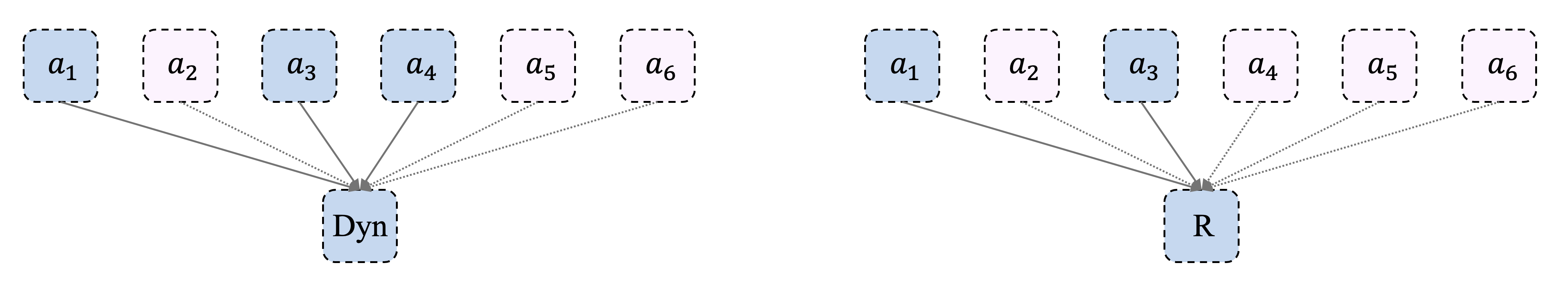
Such a problem can be addressed from the perspective of causal discovery. Formally, we can use the Structural Causal Models (SCMs) to represent the underlying causal structure of a sequential decision making process, as shown in Figure 2. Under this language, we use the notion of causal actions to denote $a_{i}^{(1,...,M)}$ , and nuisance actions for other dimension of actions. In our work, we use IC-INVASE for causal discovery. Ideally, the action selection function $G$ should be able to distinguish between nuisance action dimensions and the causal ones that has causal relation with either dynamics or reward mechanism. We present in the next section our causal discovery algorithms.

3.2 Iterative Curriculum INVASE (IC-INVASE)

Instead of directly applying INVASE to solve Equation (6). We first propose two improvements to make the vanilla INVASE more suitable for large-scale variable selection tasks as the action dimension in RL might be extremely large [33]. Specifically, the first improvement, based on curriculum learning, is introduced to tackle the exploration difficulty when $\lambda$ in Equation (1) is large, where INVASE tends to converge to poor sub-optimal solutions and prune all variables including the useful ones [37]. The second improvement is based on the iterative structure of variable selection tasks: the feature selection operator $G$ can be applied multiple times to conduct hierarchical feature selection without introducing extra computation expenses.

3.2.1 Curriculum Learning For High Dimensional Variable Selection

The work of [3] first introduces Curriculum Learning to mimic human learning by gradually learn more complex concepts or handle more difficult tasks. Effectiveness of the method has been demonstrated in various set-ups [3, 19, 7, 34, 36]. In general, it should be easier to select $M$ useful variables out of $L$ input variables when $M$ is larger. The most trivial case is to select all $L$ variables, with an identical mapping $x^{(G(x))}=G(x)\odot x=x$ . Formally, we have

Proposition 1 (Curriculum Property in Variable Selection).

Assume $M$ out of $L$ variables are outcome-related, let $M\leq N_{1}<N_{2}\leq L$ , $G_{N_{1}}(x)$ minimizes $\mathcal{D}_{KL}(p(Y|X=x)||p(Y|X^{(G(x))}=x^{(G(x))}))+\lambda||G(x)|_{0}-N_{1}|$ . Then
$G_{N_{2}}(x)$ minimizes $\mathcal{D}_{KL}(p(Y|X=x)||p(Y|X^{G(x)}=x^{G(x)}))+\lambda||G(x)|_{0}-N_{2}|$ can be get through:
$G_{N_{2}}(x)\in\{G_{N_{1}}(x)\lor[G_{N_{1}}(x)\mathbf{XOR}~{}\mathbf{1}]_{1_{N_{2}-N_{1}}}\}$ ,
where $[\cdot]_{1_{N_{2}-N_{1}}}$ means keep $N_{2}-N_{1}$ none-zero elements unchanged while replacing other elements by $0$ .

Proof.

By the definition of the $[\cdot]_{1_{N_{2}-N_{1}}}$ operator, $||G(x)|_{0}-N_{2}|=0$ is minimized. On the other hand, starting from $N_{1}=M$ , minimizing $\mathcal{D}_{KL}(p(Y|X=x)||p(Y|X^{(G(x))}=x^{(G(x))}))$ requires all the $M$ outcome-related variables being selected by $G_{N_{1}}$ . Therefore, $G_{N_{2}}$ also minimizes the KL-divergence by the independent assumption of the other $L-M$ variables with the outcomes. ∎

The proposition indicates the difficulty of selecting $N$ useful out of $L$ variables decreases monotonically as $N\geq M$ increase from $M,M+1,...,L$ . In this work, two classes of practical curriculum are designed: 1. curriculum on the $l_{0}$ penalty coefficient, and 2. curriculum on the proportion of variables to be selected.

Curriculum on $l_{0}$ Penalty Coefficient

In this curriculum design, the penalty coefficient $\lambda$ in Equation (1) is increased from $0$ to a pre-determined number (e.g., $1.0$ ). Increasing the value of $\lambda$ will lead to a larger penalty on the number of variables selected by the feature selector. Experiments in [37] has shown a large $\lambda$ always lead to a trivial selector that does not select any variable.

Curriculum on the Proportion of Selected Features

In this curriculum design, the proportion of variables to be selected, denoted by $p_{r}$ , is adjusted from the default setting $0$ to a decreasing number from a pre-determined value (e.g., $0.5$ ) to $0$ . i.e., the $l_{0}$ penalty term $\lambda|G(x)|_{0}$ in Equation (1) is revised to be $\lambda||G(x)|_{0}-d\cdot p_{r}|$ , where $d$ is the dimension of input $x$ . When the proportion is set to be $p_{r}=0.5$ , the selector will be penalized whenever less or more than half of all variables are selected. Such a curriculum design forces the feature selector to learn to select less but increasingly more important variables gradually.

Thus, we get the learning objective of curriculum-INVASE:

\mathcal{L}=\mathcal{D}_{KL}(p(Y|X=x)||p(Y|X^{(G(x))}=x^{(G(x)})))+\lambda||G(x)|_{0}-d\cdot p_{r}|.

(7)

where $\lambda$ increases from $0$ to some value and $p_{r}$ decreases from a value in $[0,1)$ to $0$ .

3.2.2 Iterative Variable Selection

The second improvement proposed in this work is based on the iterative structure of variable selection tasks. Specifically, the $G(x)$ mapping $x\in\mathcal{X}$ to $\{0,1\}^{d}$ is an iterative operator, which can be applied for multiple times to perform coarse-to-fine variable selection. Although in practice we follow [37] to apply an element-wise product in producing $x^{(G(x))}$ : $x^{(G(x))}=G(x)\odot x\in\mathcal{X}$ . In more general cases, the i-th element of $x_{i}^{(G(x))}$ is

x_{i}^{(G(x))}=\begin{cases}1,\quad\mathbf{if}\quad G_{i}(x)=1.\\ *,\quad\mathbf{if}\quad G_{i}(x)=0.\end{cases}

(8)

where $*$ can be an arbitrary identifiable indicator that represents the variable is not selected.

Algorithm 1 TD3 with TD-SWAR

Initialize critic networks

C_{\phi_{1}}

C_{\phi_{2}}

, baseline networks

B_{\psi_{1}}

B_{\psi_{2}}

and actor network

\pi_{\nu}

, IC-INVASE selector network

G_{\theta}

Initialize target networks

\phi^{\prime}_{1}\leftarrow{\phi_{1}}

\phi^{\prime}_{2}\leftarrow{\phi_{2}}

\psi^{\prime}_{1}\leftarrow{\psi_{1}}

\psi^{\prime}_{2}\leftarrow{\psi_{2}}

\nu^{\prime}\leftarrow{\nu}

Initialize replay buffer

\mathcal{B}

for

t=1,H

Interact with environment and store transition tuple

(s,a,r,s^{\prime})

\mathcal{B}

Sample mini-batch of transitions

\{(s,a,r,s^{\prime})\}

from

\mathcal{B}

Calculate perturbed next action by

\tilde{a}\leftarrow\pi_{\nu^{\prime}}(s^{\prime})+\epsilon

\epsilon

is sampled from a clipped Gaussian.

Select actions with target selector network

\tilde{a}^{(G(\tilde{a}|s^{\prime}))}\leftarrow G_{\theta^{\prime}}(\tilde{a}|s^{\prime})\odot\tilde{a}

Calculate target critic value

y_{c}

and baseline value

y_{b}

y_{c}\leftarrow r+\gamma\min_{i=1,2}C_{\phi^{\prime}_{i}}(s^{\prime},\tilde{a}^{(G(\tilde{a}|s^{\prime}))})

y_{b}\leftarrow r+\gamma\min_{i=1,2}B_{\psi^{\prime}_{i}}(s^{\prime},\tilde{a})

Update critics and baselines with selected actions:

a^{(G(a|s))}\leftarrow G_{\theta}(a|s^{\prime})\odot a

\phi_{i}\leftarrow\arg\min_{\phi_{i}}\mathbf{MSE}(y_{c},C_{\phi_{i}}(s,a^{(G(a|s))}))

\psi_{i}\leftarrow\arg\min_{\psi_{i}}\mathbf{MSE}(y_{b},B_{\psi_{i}}(s,a))

Update IC-INVASE selector network by the policy gradient, with learning rate

\eta_{1}

\theta\leftarrow\theta-\eta_{1}(l_{b}-l_{c})\nabla_{\theta}\log G_{\theta}(a|s)

l_{b}

l_{c}

are MSE losses in the previous step.

Update

\nu

by the deterministic policy gradient, with learning rate

\eta_{2}

\nu\leftarrow\nu-\eta_{2}\nabla_{a}C_{\phi_{1}}(s,a)|_{a=\pi_{\nu}(s)}\nabla_{\nu}\pi_{\nu}(s)

Update target networks, with

\tau\in(0,1)

\phi^{\prime}_{i}\leftarrow\tau{\phi_{i}}+(1-\tau)\phi^{\prime}_{i}

\psi^{\prime}_{i}\leftarrow\tau{\psi_{i}}+(1-\tau)\psi^{\prime}_{i}

\nu^{\prime}\leftarrow\tau{\nu}+(1-\tau)\nu^{\prime}

end for

On the other hand, once the outputs $G(x)$ of the selector have been recorded, $*$ can be replaced by any label-independent variable $G(x)\odot z$ , where $z\sim p_{z}(\cdot)$ is outcome-independent. Then $x^{(G(x))}$ can be regarded as a new sample and be fed into the variable selector, resulting in a hierarchical variable selection process:

\begin{array}[]{ll}&x^{(1)}=(G(x)\odot x)\oplus(G(x)\odot z),\\ &x^{(2)}=(G(x^{(1)})\odot x^{(1)})\oplus(G(x^{(1)})\odot z),\\ &...\\ &x^{(n)}=(G(x^{(n-1)})\odot x^{(n-1)})\oplus(G(x^{(n-1)})\odot z),\end{array}

(9)

where $z\sim p_{z}(\cdot)$ , and $\oplus$ is the element-wise sum operator. Moreover, if the distribution of irrelevant variable $p_{x}(\cdot)$ is known, applying the variable selection operator obtained from Equation (7) for multiple times with $p_{z}(\cdot)\buildrel d\over{=}p_{x}(\cdot)$ has the meaning of hierarchical variable selection: after each operation, the most obvious $1-p_{r}$ irrelevant variables are discarded. e.g., when $p_{r}=0.5$ , ideally top- $50\%,25\%,12.5\%$ most important variables will be selected after the first three selection operations. In this work, a coarse approximation is utilized by selecting $z$ to be $z=0$ for simplicity. ³³3 $p_{z}(\cdot)$ may be learned through generative models to approximate $p_{x}(\cdot)$ , and Equation (9) can be regarded as a kind of data-augmentation or ensemble method. This idea is left for the future work.

Combining those two improvements lead to an Iterative Curriculum version of INVASE (IC-INVASE) that addresses the exploration difficulty in high-dimensional variable selection tasks. Curriculum learning helps IC-INVASE to achieve better asymptotic performance, i.e., achieve higher True Positive Rate (TPR) and lower False Discovery Rate (FDR), while iterative application of the selection operator contributes to higher learning efficiency: selectors models with different level of TPR/FDR can be generated on-the-fly.

3.3 State-Wise Action Refinery with IC-INVASE

3.3.1 Temporal Difference State-Wise Action Refinery

With the techniques introduced in the previous section, higher dimensional variable selection tasks can be better solved, therefore we are ready to use IC-INVASE to solve Equation (6). The resulting algorithm is called Temporal Difference State-Wise Action Refinery (TD-SWAR).

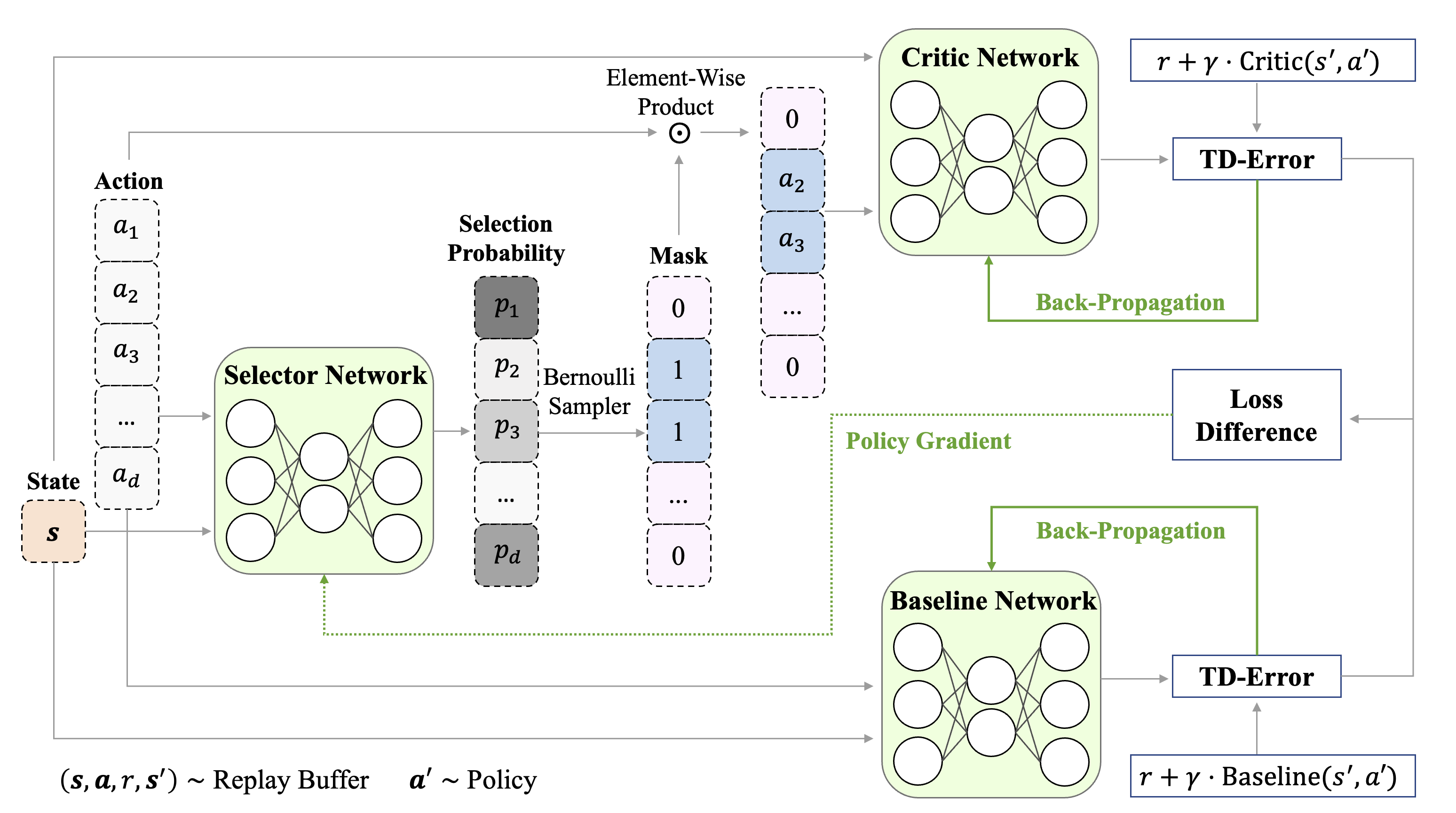
In this work, TD3 [10] is used as the basic algorithm we build TD-SWAR up on. In addition to the policy network $\pi_{\nu}$ , double critic networks $C_{\phi_{1}}$ , $C_{\phi_{2}}$ and their corresponding target networks used in vanilla TD3, TD-SWAR includes an action selector model $G_{\theta}$ and two baseline networks $B_{\psi_{1}}$ , $B_{\psi_{2}}$ following [37] to reduce the variance in policy gradient learning. Pseudo-code for the proposed algorithm is shown in Algorithm 1. And the block diagram in Figure 1 illustrates how different modules in TD-SWAR updates their parameters.

3.3.2 Static Approximation: Model-Based Action Selection

While IC-INVASE can be formally integrated with temporal difference learning, the learning stability is not guaranteed. Different from general regression tasks where the label for every instance is fixed across training, in temporal difference learning, the regression target is closely related to the present critic function $C_{\phi}$ , the policy $\pi_{\nu}$ that generates the transition tuples used for training, and the selector model of IC-INVASE itself. In this section, a static approach is proposed to approximately solve the challenge of instability in TD-SWAR ⁴⁴4Analysis on the approximation is provided in Appendix A.

Other than applying the IC-INVASE algorithm to solve Equation (6), another way of leveraging IC-INVASE in action space pruning is to combine it with the model-based methods [11, 16, 13, 14], where a dynamic model $\mathcal{P}:\mathcal{S}\times\mathcal{A}\mapsto\mathcal{S}$ is learned through regression:

\mathcal{P}=\arg\min_{\mathcal{P}}\mathbb{E}_{(s,a,s^{\prime})\sim\pi,\mathcal{T}}(s^{\prime}-\mathcal{P}(s,a))^{2}

(10)

Although the task of precise model-based prediction is in general challenging [24], in this work, we only adopt model-based prediction in action selection, and the target is action discovery other than precise prediction. As the dynamic models are always static across learning, such an approach can be much more stable than TD-SWAR. We name this method as Dyn-SWAR and present the pseudo-code in Algorithm 2, where we infuse IC-INVASE to Equation (10) and get the learning objective:

\min_{G,\mathcal{P}}\mathbb{E}_{(s,a,s^{\prime})\sim\pi,\mathcal{T}}(s^{\prime}-\mathcal{P}(s,a^{(G(a|s))}))^{2}

(11)

4 Experiment

Algorithm 2 TD3 with Dyn-SWAR

Initialize critic networks

Q_{w_{1}}

Q_{w_{2}}

, Dynamics critic model

C_{\phi}

, dynamic baseline model

B_{\psi}

, actor network

\pi_{\nu}

, and IC-INVASE selector network

G_{\theta}

Initialize target networks

w^{\prime}_{1}\leftarrow{w_{1}}

w^{\prime}_{2}\leftarrow{w_{2}}

\nu^{\prime}\leftarrow{\nu}

Initialize replay buffer

\mathcal{B}

for

t=1,H

Interact with environment and store transition tuple

(s,a,r,s^{\prime})

\mathcal{B}

Sample mini-batch of transitions

\{(s,a,r,s^{\prime})\}

from

\mathcal{B}

Update dynamic critics and dynamic baselines with equation (10):

\phi\leftarrow\arg\min_{\phi}\mathbf{MSE}(s^{\prime},C_{\phi}(s,a^{(G(a|s))}))

\psi\leftarrow\arg\min_{\psi}\mathbf{MSE}(s^{\prime},B_{\psi}(s,a))

Update IC-INVASE selector network by the policy gradient, with learning rate

\eta_{1}

\theta\leftarrow\theta-\eta_{1}(l_{b}-l_{c})\nabla_{\theta}\log G_{\theta}(a|s)

l_{b}

l_{c}

are MSE losses in the previous step.

Calculate perturbed next action by

\tilde{a}\leftarrow\pi_{\nu^{\prime}}(s^{\prime})+\epsilon

\epsilon

is sampled from a clipped Gaussian.

Select actions with selector network

\tilde{a}^{(G(\tilde{a}|s^{\prime}))}\leftarrow G_{\theta^{\prime}}(\tilde{a}|s^{\prime})\odot\tilde{a}

Calculate target critic value

y

and update critic networks:

y\leftarrow r+\gamma\min_{i=1,2}Q_{w^{\prime}_{i}}(s^{\prime},\tilde{a}^{(G(\tilde{a}|s^{\prime}))})

w_{i}\leftarrow\arg\min_{w_{i}}\mathbf{MSE}(y,Q_{w_{i}}(s,a^{(G(a|s))}))

Update

\nu

by the deterministic policy gradient, with learning rate

\eta_{2}

\nu\leftarrow\nu-\eta_{2}\nabla_{a}Q_{w_{1}}(s,a)|_{a=\pi_{\nu}(s)}\nabla_{\nu}\pi_{\nu}(s)

Update target networks, with

\tau\in(0,1)

w^{\prime}_{i}\leftarrow\tau{w_{i}}+(1-\tau)w^{\prime}_{i}

\nu^{\prime}\leftarrow\tau{\nu}+(1-\tau)\nu^{\prime}

end for

In this section, we demonstrate our proposed methods in five continuous control RL tasks with redundant action space where our proposed methods can perform causality-aware RL. We provide quantitatively comparison between IC-INVASE and the vanilla INVASE on synthetic datasets to show its improved scalability in Appendix B.

Table 1: Tasks used in evaluating SWAR in temporal difference learning

Task/Dimension	$\|\mathcal{S}\|$	$\|\mathcal{A}\|$	$\|\mathcal{A}_{red.}\|$
Pendulum-v0	3	1	100
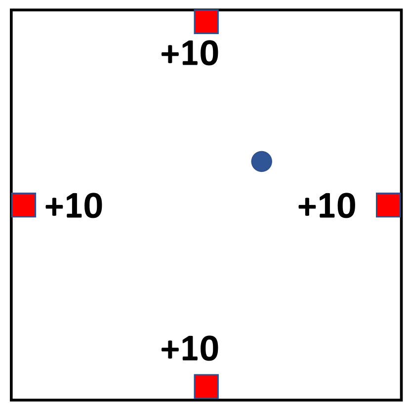
FourRewardMaze	2	2	100
LunarLanderContinuous-v2	8	2	100
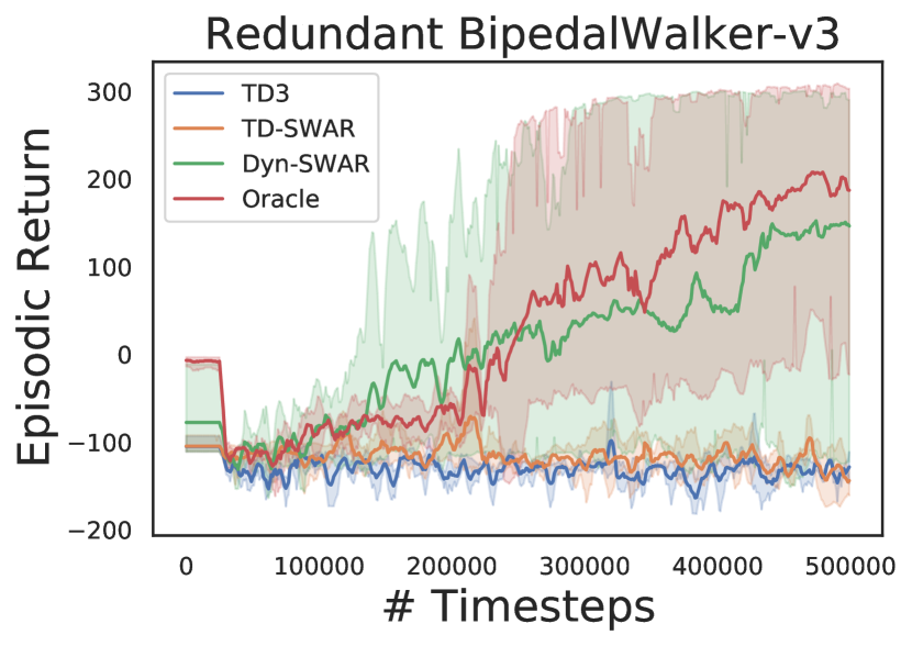
BipedalWalker-v3	24	4	100
Walker2d-v2	17	6	100

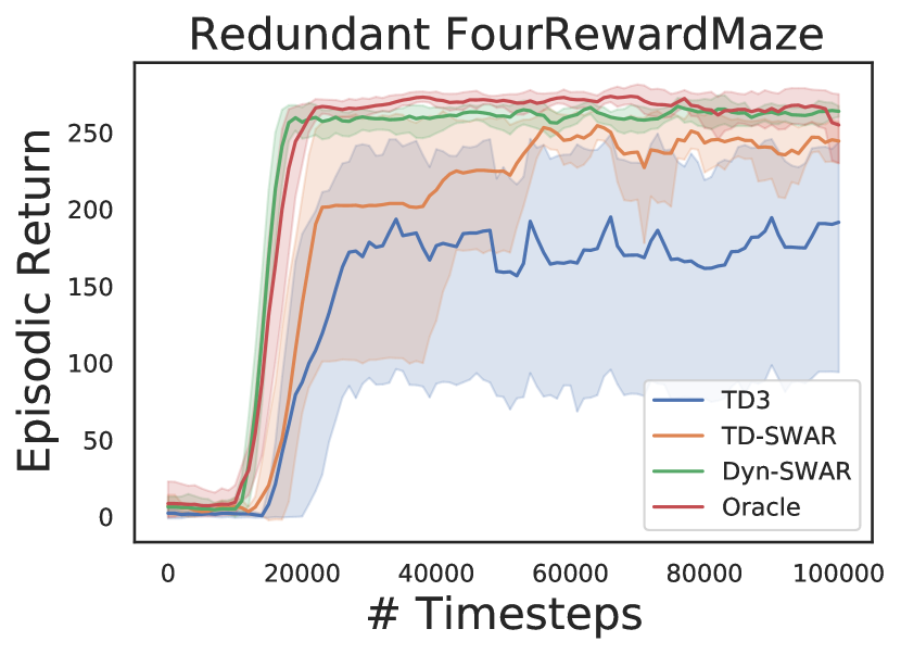
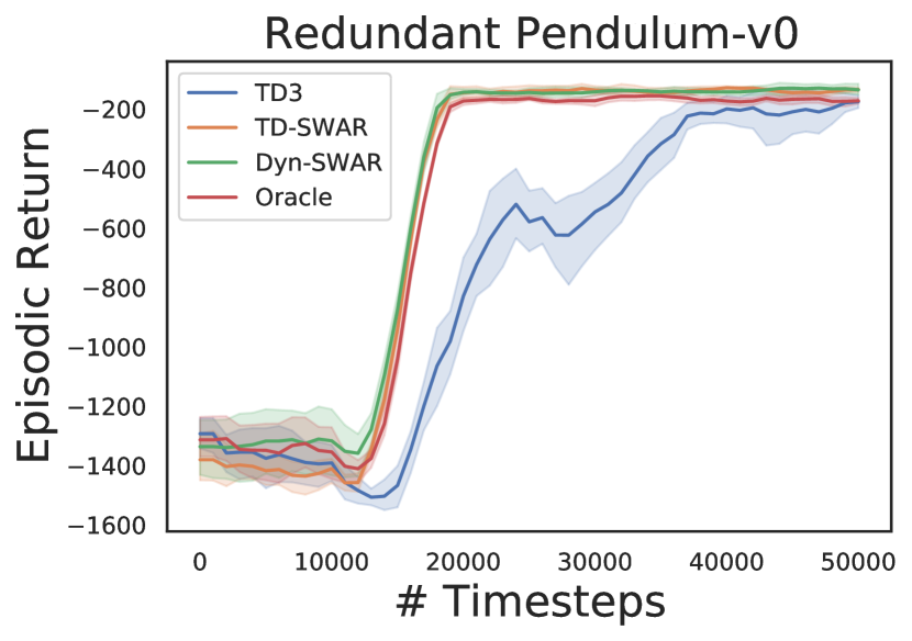
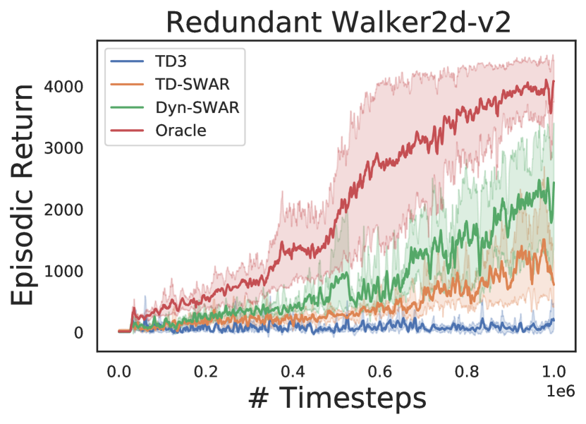
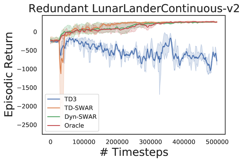
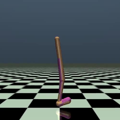
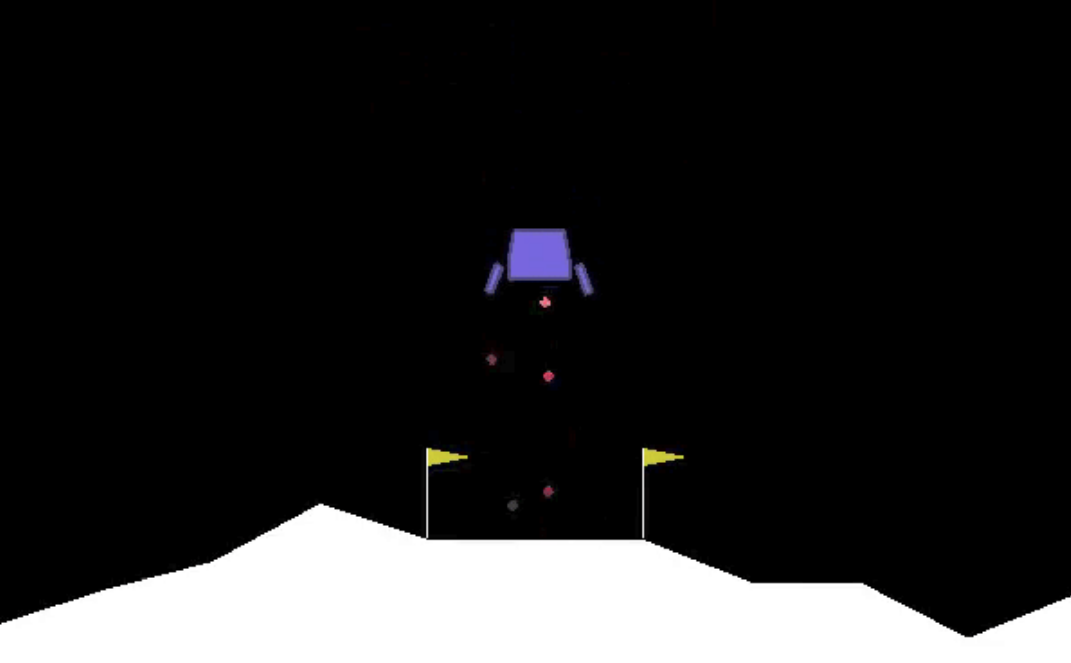
For this set of experiments, we use five RL environments (Figure 5) that are listed in Table 1 ⁵⁵5For more details of the environments please refer to Appendix C. $|\mathcal{S}|$ means the dimension of state space in each task, $|\mathcal{A}|$ represents the dimension of task-related action space, and $|\mathcal{A}_{red.}|$ indicates the dimension of redundant action space that is injected to each task. Those redundant dimensions of actions will not affect the state transitions or reward calculation, but an agent needs to learn to identify those redundant dimensions to perform efficient learning.

We evaluate both TD-SWAR that integrate IC-INVASE with temporal difference learning and its static variant Dyn-SWAR that applies IC-INVASE in dynamics prediction. The results are compared with two baselines: the Oracle: redundant action dimensions are eliminated manually; and TD3: the vanilla TD3 algorithm without explicit action redundancy reduction.

In experiments, we find the implementation of Dyn-SWAR can be much more efficient in terms of both sample complexity and computational expense: while the TD-SWAR need to continuously update all parameters for the IC-INVASE selector to keep consistent with the real-time policy and value networks as the regression label varies along time, the Dyn-SWAR selector can be trained with far less amount of data. Say, $10,000$ to $25,000$ timesteps of interactions with the environment. Such a property can be naturally combined with the warm-up trick used in TD3 [10], i.e., the Dyn-SWAR selector can be trained with warm-up transition tuples collected in the random exploration phase and then be fixed in the later learning process. Compared with normal RL settings where millions of interactions with the environment are always needed, the training of Dyn-SWAR only increases negligible computational expense.

The results are shown in Figure 4. In all environments, agent learning with IC-INVASE in both manner (TD-/Dyn-) outperforms the vanilla TD3 baseline. The Dyn-SWAR achieves high learning efficiency that is comparable to the oracle benchmarks. However, the performance of TD-SWAR in higher dimensional tasks (Walker2d-v2 and BipedalWalker-v3) still has a lot of room for improvement. Improving the stability of and scalability of instance-wise variable selection in temporal difference learning thereby should be addressed in future work.

5 Related Work

Instance-Wise Feature Selection

While traditional feature selection method like LASSO [30] aims at finding globally important features across the whole dataset, instance-wise feature selection try to discover the feature-label dependency on a case-by-case basis. L2X [5] performs instance-wise feature selection through mutual information maximization with the technique of Gumbel softmax. L2X requires pre-determined hyper-parameter $k$ to indicate how many features should be selected for each instance, which limits its performance while the number of label-relevant features varies across instances.

In this work, we build our instance-wise action selection model on top of INVASE [37], where policy gradient is applied to replace the Gumbel softmax trick and the size of chosen features per instance is more flexible. [31] considers instance-wise feature selection problems in time-series setting, and build generative models to capture counterfactual effects in time series data. Their work enables evaluation of the importance of features over time, which is crucial in the context of healthcare. [18] formally defines different types of feature redundancy and leverages mutual information maximization in instance-wise feature group discovery and introduces theoretical guidance to find the optimal number of different groups.

Our work is distinguished from previous works for instance-wise feature selection in two aspects. First, while previous works focus on static scenarios like classification and regression, this work focus on temporal difference learning where there is no static label. Second, the scalability of previous methods in variable selection is challenged as there might exist hundreds of redundant actions in the context of RL.

Dimension Reduction in RL

In the context of RL, attention models [32] have been applied to interpret the behaviors of learned policies. [29] proposes to perceive the state information through a self-attention bottleneck in vision-based RL tasks, which concentrates on the state space redundancy reduction with image inputs. The work of [22] also applies the attention mechanism to learn task-relevant information. The proposed method achieves state-of-the-art performance on Atari games with image input while being more understandable with top-down attention models.

Different from those papers, this work considers relatively tight state representations (vector input), and focuses on the task-irrelevant action reduction. We aim at finding the task-related actions and improving the learning efficiency without wasting samples in learning the task-irrelevant dimensions of actions. Our work is most closely related to AE-DQN [38] in that we both consider the problem of redundant action elimination. AE-DQN tackles action space redundancy with an action-elimination network that eliminates sub-optimal actions. Yet its discussion is limited in the discrete settings. In contrast, our work focuses on action elimination in continuous control tasks.

6 Conclusion and Future Work

In this work, we tackle the challenge of action space pruning in action redundant RL tasks. Recent advance on instance-wise feature selection technique (INVASE) is exploited after curriculum learning and iterative operation are integrated for the pursuance of scalability and efficiency. The resulting method, termed IC-INVASE, is then generalized to the RL setting where two different algorithms are proposed, TD-SWAR and Dyn-SWAR, to conduct causality-aware RL. While the former algorithm addresses the action redundant issue directly in temporal difference learning, the latter algorithm captures dynamical causality with model-based prediction. Experiments on various tasks demonstrate the causality-awareness is crucial for RL agents to perform efficient learning in action-redundant environments.

In future work, the iterative property can be further explored to perform ensemble methods in variable selection. And a more proper curriculum might be designed to better fuse multiple curricula together. On the RL side, the stability of TD-SWAR might be further improved for better sample efficiency.

References

Abadi et al. [2016] Martín Abadi, Paul Barham, Jianmin Chen, et al. Tensorflow: A system for large-scale machine learning. In OSDI, 2016.
Andrychowicz et al. [2020] OpenAI: Marcin Andrychowicz, Bowen Baker, Maciek Chociej, et al. Learning dexterous in-hand manipulation. IJRR, 2020.
Bengio et al. [2009] Yoshua Bengio, Jérôme Louradour, et al. Curriculum learning. In ICML, 2009.
Berner et al. [2019] Christopher Berner, Greg Brockman, Brooke Chan, et al. Dota 2 with large scale deep reinforcement learning. arXiv:1912.06680, 2019.
Chen et al. [2018] Jianbo Chen, Le Song, et al. Learning to explain: An information-theoretic perspective on model interpretation. arXiv:1802.07814, 2018.
Chollet and others [2015] François Chollet et al. Keras. https://github.com/fchollet/keras, 2015.
Czarnecki et al. [2018] Wojciech Marian Czarnecki, Siddhant M Jayakumar, Max Jaderberg, et al. Mix&match-agent curricula for reinforcement learning. arXiv:1806.01780, 2018.
de Haan et al. [2019] Pim de Haan, Dinesh Jayaraman, and Sergey Levine. Causal confusion in imitation learning. In NeurIPS, pages 11698–11709, 2019.
Even-Dar et al. [2006] Eyal Even-Dar, Shie M., et al. Action elimination and stopping conditions for the multi-armed bandit and reinforcement learning problems. JMLR, 2006.
Fujimoto et al. [2018] Scott Fujimoto, Herke Van Hoof, and David Meger. Addressing function approximation error in actor-critic methods. arXiv:1802.09477, 2018.
Ha and Schmidhuber [2018] David Ha and Jürgen Schmidhuber. World models. arXiv:1803.10122, 2018.
Haarnoja et al. [2018] Tuomas Haarnoja, Aurick Zhou, et al. Soft actor-critic: Off-policy maximum entropy deep reinforcement learning with a stochastic actor. arXiv:1801.01290, 2018.
Hafner et al. [2019] Danijar Hafner, Timothy Lillicrap, Jimmy Ba, et al. Dream to control: Learning behaviors by latent imagination. arXiv:1912.01603, 2019.
Janner et al. [2019] Michael Janner, Justin Fu, Marvin Zhang, et al. When to trust your model: Model-based policy optimization. In NeurIPS, 2019.
Konda and Tsitsiklis [2000] Vijay R Konda and John N Tsitsiklis. Actor-critic algorithms. In NeurIPS, 2000.
Langlois et al. [2019] Eric Langlois, Shunshi Zhang, Guodong Zhang, et al. Benchmarking model-based reinforcement learning. arXiv:1907.02057, 2019.
Lillicrap et al. [2015] Timothy P Lillicrap, Jonathan J Hunt, Alexander Pritzel, et al. Continuous control with deep reinforcement learning. arXiv:1509.02971, 2015.
Masoomi et al. [2020] Aria Masoomi, Chieh Wu, Tingting Zhao, et al. Instance-wise feature grouping. NeurIPS, 2020.
Matiisen et al. [2019] Tambet Matiisen, Avital Oliver, et al. Teacher-student curriculum learning. TNNLS, 2019.
[20] Andrew Melnik, Luca Lach, Matthias Plappert, et al. Tactile sensing and deep reinforcement learning for in-hand manipulation tasks.
Mnih et al. [2015] Volodymyr Mnih, Koray Kavukcuoglu, David Silver, et al. Human-level control through deep reinforcement learning. Nature, 2015.
Mott et al. [2019] Alexander Mott, Daniel Zoran, et al. Towards interpretable reinforcement learning using attention augmented agents. In NeurIPS, 2019.
Paszke et al. [2017] Adam Paszke, Sam Gross, Soumith Chintala, et al. Automatic differentiation in pytorch. 2017.
Sharma et al. [2019] Archit Sharma, Shixiang Gu, Sergey Levine, et al. Dynamics-aware unsupervised discovery of skills. arXiv:1907.01657, 2019.
Silver et al. [2014] David Silver, Guy Lever, et al. Deterministic policy gradient algorithms. In ICML, 2014.
Silver et al. [2016] David Silver, Aja Huang, Chris J Maddison, et al. Mastering the game of go with deep neural networks and tree search. nature, 2016.
Sun et al. [2018] Peng Sun, Xinghai Sun, Lei Han, et al. Tstarbots: Defeating the cheating level builtin ai in starcraft ii in the full game. arXiv:1809.07193, 2018.
Sutton and Barto [1998] Richard S Sutton and Andrew G Barto. Reinforcement learning: An introduction. 1998.
Tang et al. [2020] Yujin Tang, Duong Nguyen, and David Ha. Neuroevolution of self-interpretable agents. arXiv:2003.08165, 2020.
Tibshirani [1996] Robert Tibshirani. Regression shrinkage and selection via the lasso. JRSS, 1996.
Tonekaboni et al. [2020] Sana Tonekaboni, S. Joshi, et al. What went wrong and when? instance-wise feature importance for time-series black-box models. NeurIPS, 2020.
Vaswani et al. [2017] Ashish Vaswani, Noam Shazeer, et al. Attention is all you need. In NeurIPS, 2017.
Vinyals et al. [2019] Oriol Vinyals, Igor Babuschkin, Wojciech M Czarnecki, et al. Grandmaster level in starcraft ii using multi-agent reinforcement learning. Nature, 2019.
Weinshall et al. [2018] Daphna Weinshall, Gad Cohen, et al. Curriculum learning by transfer learning: Theory and experiments with deep networks. arXiv:1802.03796, 2018.
Williams [1992] Ronald J Williams. Simple statistical gradient-following algorithms for connectionist reinforcement learning. Machine learning, 8(3-4):229–256, 1992.
Xu et al. [2020] Benfeng Xu, L. Zhang, et al. Curriculum learning for natural language understanding. In ACL, 2020.
Yoon et al. [2018] Jinsung Yoon, James Jordon, and Mihaela van der Schaar. Invase: Instance-wise variable selection using neural networks. In ICLR, 2018.
Zahavy et al. [2018] Tom Zahavy, Matan Haroush, et al. Learn what not to learn: Action elimination with deep reinforcement learning. In NeurIPS, 2018.

Appendix A On the Dynamic Model Approximation

We provide analysis on the approximation in this section based on the deterministic MDP model in finite action space where the problem degenerates to $Q$ -Learning. Similar results can be get to prove the Policy Evaluation Lemma, combined with Policy Improvement Lemma (given proper function approximation of the $\arg\max$ operator) and result in Policy Iteration Theorem.

In deterministic MDPs with $s_{t+1}=\mathcal{T}(s_{t},a_{t})$ , $r_{t}=r(s_{t},a_{t})$ , the value function of a state is defined as

V^{\pi}(s)=\sum_{t=0}^{\infty}\gamma^{t}r(s_{t},a_{t}),

(12)

given $s_{0}=s$ is the initial state and $a_{t}=\pi(s_{t})$ comes from the deterministic policy $\pi$ .

The learning objective is to find an optimal policy $\pi$ , such that an optimal state value can be achieved:

V^{*}(s)=\max_{\pi}V^{\pi}(s)

(13)

The state-action value function ( $Q$ -function) is then defined as

Q(s,a)=r(s,a)+\gamma V^{*}(\mathcal{T}(s,a))

(14)

Formally, the objective of action space pruning in action-redundant MDPs is to find an optimal policy $\pi^{(G)}=G(\pi(s_{t})|s_{t})\odot\pi(s_{t})$ with an action selector $G:\mathcal{S}\times\mathcal{A}\mapsto\{0,1\}^{d}$ ,

V^{*}(s)=\max_{\pi^{(G)}}V^{\pi^{(G)}}(s)=\max_{\pi}V^{\pi}(s),

(15)

with minimal number of actions selected, i.e., $|G|_{0}$ is minimized. The sufficient and necessary condition for Equation (15) to hold is $r(s_{t},\pi(s_{t}))=r(s_{t},\pi^{(G)}{(s_{t})})$ and $\mathcal{T}(s_{t},\pi(s_{t}))=\mathcal{T}(s_{t},\pi^{(G)}(s_{t}))$ .

In general, the reward function $r$ and transition dynamics $\mathcal{T}$ may depend on different subsets of actions and the optimal, i.e., $r(s_{t},a_{t})=r(s_{t},a_{t}^{(G_{1})})$ , while $\mathcal{T}(s_{t},a_{t})=\mathcal{T}(s_{t},a_{t}^{(G_{2})})$ , where $G_{1}$ , $G_{2}$ select different subset of given actions by $a_{t}^{(G_{1})}=G_{1}(a_{t}|s_{t})\odot a_{t}$ , $a_{t}^{(G_{2})}=G_{2}(a_{t}|s_{t})\odot a_{t}$ but $a_{t}^{(G_{1})}\neq a_{t}^{(G_{2})}$ . The final action selector $G$ should be generated according to $G(a|s)=G_{1}(a|s)\lor G_{2}(a|s)$ , where $\lor$ is the element-wise $\mathbf{OR}$ operation.

Therefore, in our approximation of Dyn-SWAR, we assume $G(a|s)=G_{2}(a|s)$ as an approximation for $G(a|s)=G_{1}(a|s)\lor G_{2}(a|s)$ . Future work may include another predictive model for the reward function and take the element-wise $\mathbf{OR}$ operation to get $G$ .

Appendix B Additional Experiments

B.1 Synthetic Data Experiment

The synthetic datasets are generated in the same way as [5, 37]. Specifically, there are $6$ synthetic datasets that have inputs generated from an $11$ -dim Gaussian distribution without correlations across features. The label $Y$ for each dataset is generated by a Bernoulli random variable with $P(Y=1|X)=\frac{1}{1+\text{logit}(X)}$ . In different tasks, $\text{logit}(X)$ takes the value of:

•

$\mathbf{Syn1}$ : $\exp(X_{1}X_{2})$
•

$\mathbf{Syn2}$ : $\exp(\sum_{i=3}^{6}X_{i}^{2}-4)$
•

$\mathbf{Syn3}$ : $-10\times\sin{2X_{7}}+2|X_{8}|+X_{9}+\exp(-X_{10})$
•

$\mathbf{Syn4}$ : if $X_{11}<0$ , logit follows $\mathbf{Syn1}$ , otherwise, logit follows $\mathbf{Syn2}$
•

$\mathbf{Syn5}$ : if $X_{11}<0$ , logit follows $\mathbf{Syn1}$ , otherwise, logit follows $\mathbf{Syn3}$
•

$\mathbf{Syn6}$ : if $X_{11}<0$ , logit follows $\mathbf{Syn2}$ , otherwise, logit follows $\mathbf{Syn3}$

In the first three synthetic datasets, the label $Y$ depends on the same feature across each dataset, while in the last three datasets, the subsets of features that label $Y$ depends on are determined by the values of $X_{11}$ .

For each dataset, $20,000$ samples are generated and be separated into a training set and a testing set. In this work, we focus on finding outcome-relevant features (e.g., finding task-relevant actions in the context of RL), thus the true positive rate (TPR) and false discovery rate (FDR) are used as performance metrics.

11-dim Feature Selection

Table 2 shows the quantitative results of the proposed method, IC-INVASE on the 11-dim feature selection tasks. To accelerate training and facilitate the usage of dynamical computational graphs in curriculum learning and RL settings, the vanilla INVASE is re-implemented with PyTorch [23]. In general, the PyTorch implementation is $4$ to $5$ times faster than the previous Keras [1, 6] implementation, with on-par performance on the $11$ -dim feature selection tasks. In the comparison, both the reported results in [37] (denoted by INVASE (REP.)) and our experimental results on INVASE (denoted by INVASE (EXP.)) are presented. The $p_{r}$ curriculum for IC-INVASE in all experiments are set to decrease from $0.5$ to $0.0$ except in ablation studies. Results of two different choices of the $\lambda$ curriculum are reported and denoted by IC-INVASE ( $\mathbf{\lambda\uparrow\cdot}$ ), e.g., $\lambda\uparrow 0.3$ means $\lambda$ increases from $0.0$ to $0.3$ in the experiment. We omit the results on the first three datasets ( $\mathbf{Syn1}$ , $\mathbf{Syn2}$ , $\mathbf{Syn3}$ ) where both IC-INVASE and INVASE achieve $100.0$ TPR and $0.0$ FDR. Iteration $1$ to Iteration $4$ in the table shows the results after applying the selection operator for different number of iterations.

In all experiments, IC-INVASE achieves better performance (i.e., larger TPR and lower FDR) than the vanilla INVASE with Keras and PyTorch implementation. Iterative applying the feature selection operator can reduce the FDR with a slight cost of TPR decay.

100-dim Feature Selection

We then increase the total number of feature dimensions to $100$ to demonstrate how IC-INVASE improves the vanilla INVASE in larege-scale variable selection settings. In this experiment. The features are generated with $100$ -dim Gaussian without correlations and the rules for label generation are still the same as the $11$ -dim settings. (i.e., $89$ additional label-independent noisy dimensions of input is concatenated to the $11$ -dim inputs.)

The results are shown in Table 3. IC-INVASE achieves much better performance in all datasets, i.e., higher TPR and lower FDR. The ablation studies on different curriculum show both an increasing $\lambda$ and a decreasing $p_{r}$ can benefit discovery of label-dependent features. As the hyper-parameters for curriculum are not elaborated in our experiments, direct combining the two curriculum may hinder the performance. The design for curriculum fusion is left to the future work.

Table 2: Relevant variables discovery results for Synthetic datasets with 11-dim input

Data Set	Method	Iteration $1$		Iteration $2$		Iteration $3$		Iteration $4$
Metric		TPR	FDR	TPR	FDR	TPR	FDR	TPR	FDR
$\mathbf{Syn4}$	INVASE (rep.)	99.8	10.3
	INVASE (exp.)	98.6	1.6	98.1	1.1	98.1	1.1	98.1	1.1
	IC-INVASE ( $\lambda\uparrow 0.2$ )	99.7	3.4	99.7	2.6	99.7	2.5	99.7	2.5
	IC-INVASE ( $\lambda\uparrow 0.3$ )	99.3	1.6	99.3	0.8	99.3	0.8	99.3	0.8
$\mathbf{Syn5}$	INVASE (rep.)	84.8	1.1
	INVASE (exp.)	82.1	1.0	79.7	1.0	79.3	1.0	79.2	1.0
	IC-INVASE ( $\lambda\uparrow 0.2$ )	99.3	1.6	99.1	1.1	99.1	1.1	99.1	1.1
	IC-INVASE ( $\lambda\uparrow 0.3$ )	96.8	1.0	96.4	0.4	96.4	0.4	96.4	0.4
$\mathbf{Syn6}$	INVASE (rep.)	90.1	7.4
	INVASE (exp.)	92.3	1.7	89.8	1.6	89.6	1.6	89.6	1.6
	IC-INVASE ( $\lambda\uparrow 0.2$ )	99.6	2.9	99.5	2.6	99.5	2.5	99.5	2.5
	IC-INVASE ( $\lambda\uparrow 0.3$ )	99.4	1.9	99.3	1.6	99.3	1.6	99.3	1.6

Table 3: Relevant feature discovery results for Synthetic datasets with 100-dim input

Data Set	Method	Iteration $1$		Iteration $2$		Iteration $3$		Iteration $4$
Metric		TPR	FDR	TPR	FDR	TPR	FDR	TPR	FDR
$\mathbf{Syn4}$	INVASE (rep.)	66.3	40.5
	INVASE (exp.)	27.0	6.5	18.0	6.4	18.0	6.4	18.0	6.4
	IC-INVASE W/O $p_{r}\downarrow$	66.3	40.5	66.3	40.5	66.3	40.5	66.3	40.5
	IC-INVASE W/O $\lambda\uparrow$	100.0	43.0	100.0	43.0	100.0	43.0	100.0	43.0
	IC-INVASE	100.0	43.0	100.0	43.0	100.0	43.0	100.0	43.0
$\mathbf{Syn5}$	INVASE (rep.)	73.2	23.7
	INVASE (exp.)	56.4	37.9	56.4	37.9	56.4	37.9	56.4	37.9
	IC-INVASE W/O $p_{r}\downarrow$	90.9	7.8	88.8	4.4	88.8	4.3	88.8	4.3
	IC-INVASE W/O $\lambda\uparrow$	96.1	11.3	95.2	8.2	95.5	8.1	95.5	8.1
	IC-INVASE	91.9	8.1	90.8	4.3	90.8	4.2	90.8	4.2
$\mathbf{Syn6}$	INVASE (rep.)	90.5	15.4
	INVASE (exp.)	90.1	43.7	90.1	43.7	90.1	43.7	90.1	43.7
	IC-INVASE W/O $p_{r}\downarrow$	98.5	4.1	98.4	2.4	98.4	2.3	98.4	2.3
	IC-INVASE W/O $\lambda\uparrow$	99.6	8.1	99.6	7.1	99.6	7.0	99.6	7.0
	IC-INVASE	98.9	7.0	98.9	5.0	98.9	4.9	98.9	4.9

Appendix C Environment Details

FourRewardMaze

The FourRewardMaze is a 2-D navigation task where an agent need to find all four solutions to achieve better performance. The state space is $2$ -D continuous vector indicating the position of the agent, while the action space is a $2$ -D continuous value indicating the direction and step length of the agent, which is limited to $[-1,1]$ . The initial location of the agent is randomly selected for each game, and each episode has the length of $32$ , which is the timesteps needed to collect all four rewards from any starting position.

Pendulum-v0

The Pendulum-v0 environment is a classic problem in the control literature. In the Pendulum-v0 of OpenAI Gym. The task has $3$ -D state space and $1$ -D action space. In every episode the pendulum starts in a random position, and the learning objective is to swing the pendulum up and keep it staying upright.

Walker2d-v2

The Walker2d-v2 environment is a locomotion task where the learning objective is to make a two-dimensional bipedal robot walk forward as fast as possible. The task has $17$ -D state space and $6$ -D action space.

LunarLanderContinuous-v2

In the tasks of LunarLanderContinuous-v2, the agent is asked to control a lander to move from the top of the screen to a landing pad located at coordinate $(0,0)$ . The fuel is infinite, so an agent can learn to fly and then land on its first attempt. The state is as $8$ -D real-valued vector and action is $2$ -D vector in the range of $[-1,1]$ , where the first dimension controls main engine, $[-1,0]$ off, $[0.,1]$ throttle from $50\%$ to $100\%$ power and the second value in $[-1,-0.5]$ will fire left engine, while a value in $[0.5,1.0]$ fires right engine, otherwise the engine is off.

BipedalWalker-v3

The BipedalWalker-v3 is a locomotion task where the state space is $24$ -D and the action space is $4$ -D. The agent needs to walk as far as possible in each episode where a total timestep of $1000$ are given and total $300$ points might be collected up to the far end. If the robot falls, it gets $-100$ points. Applying motor torque costs a small amount of points, more optimal agent will get better score.

Appendix D Reproduction Checklist

D.1 Neural Network Structure

In all experiments, we use the same neural network structure: in TD3, we follow the vanilla implementation to use $3$ -layer fully connected neural networks where $256$ hidden units are used. In the selector networks of the INVASE module, we follow the vanilla implementation to use $3$ -layer fully connected neural networks where $100$ , $200$ hidden units are used.

D.2 Hyper-Parameters

In both TD-SWAR and the Dyn-SWAR, we apply IC-INVASE with $p_{r}$ reducing from $0.5$ to $0.0$ and $\lambda$ increasing from $0.0$ to $0.2$ . While our experiments have already shown the effectiveness and robustness of those hyper-parameters, performing grid search on those hyper-parameters may lead to further performance improvement.

Toward Causal-Aware RL: State-Wise Action-Refined Temporal Difference