Toroidal Magnetic Flux Budget in Mean-Field Dynamo Model of Solar Cycles 23 and 24
Abstract
We study the toroidal magnetic flux budget of the axisymmetric part of a 3D mean-field dynamo model of Solar Cycles 23 and 24. The model simulates the global solar dynamo that includes effects of the formation and evolution of bipolar magnetic regions emerging on the solar surface. Our analysis shows that the hemispheric magnitude of the net axisymmetric toroidal magnetic field in the bulk of the convection zone is partly defined by the surface parameters of the differential rotation and the axisymmetric radial magnetic field. The contribution of the rotational radial shear to the net axisymmetric toroidal field production has the same magnitude and it goes nearly sin-phase with the effect of the latitudinal differential rotation. For our model, the effect of the radial shear to the net axisymmetric toroidal magnetic field is determined mostly by the near equatorial regions that are slightly above and below the bottom of the convection zone. Also, we find that the toroidal field generation rate depends strongly on the latitudinal profile of the axisymmetric radial magnetic field near the poles. We find that the magnitude of the axisymmetric toroidal flux generation rate in the 3D dynamo model is by about 10 percent higher than in the axisymmetric 2D mean-field dynamo model, due to the bipolar active regions.
1 Introduction
The total unsigned radial magnetic flux observed in the photosphere during the Sun’s 11-year activity cycle peaks at about Mx (Schrijver & Harvey, 1984, 1994). Some portion of this magnetic flux is likely produced by the large-scale dynamo in the convection zone. But how and where this flux is produced is under debate. A small fraction of it comes from active regions. Depending on the complexity of active regions, the total unsigned radial magnetic field flux associated with the bipolar sunspot groups (hereafter, bipolar magnetic regions, BMRs) peaks at about - Mx (Nagovitsyn et al., 2016; Abramenko et al., 2023). A part of this flux must participate in the surface flux transport and turbulent processes, e.g., via helical convection motion, contributing to the global dynamo. Following the basic ideas of Parker (1955), the solar dynamo cyclically transforms the large-scale poloidal magnetic field into the toroidal field and back by means of the differential rotation and the turbulent effect caused by the cyclonic convective motions. Cameron & Schüssler (2015) (hereafter CS15) showed that the hemispheric magnitude of the net axisymmetric toroidal flux production in the bulk of the convection zone is largely determined by the surface parameters of the differential rotation and the radial magnetic field. Using solar observations, they found that the toroidal flux generation rate by the latitudinal rotational shear is about Mx/yr or Mx/s. Therefore, this effect is capable of producing the toroidal flux of Mx during the solar cycles. It is interesting to compare this number with the typical unsigned radial magnetic field flux emergence rate of BMRs, which is about Mx/s (Golovko, 1998). Following the arguments of CS15, it is tempting to conclude that the poloidal magnetic flux produced by the magnetic flux of bipolar magnetic regions (BMRs) is sufficient for maintaining the solar dynamo. Indeed, this idea has been implemented in the Babcock-Leighton flux transport dynamo models (Babcock, 1961; Leighton, 1969; Hazra et al., 2023; Cameron & Schüssler, 2023). It is worth noting that the evidences found by CS15 reflect effects of the global axisymmetric dynamo inside the Sun. Our aim is to analyze these effects using the 3D mean-field dynamo model developed by Pipin (2022); Pipin et al. (2023) (hereafter, \al@P22,PKT23; \al@P22,PKT23).
Despite the simplicity and visual appeal of the magnetic ‘butterfly’ diagram reproduced by the Babcock-Leighton flux transport dynamo models, this dynamo scenario is not supported by the global-Sun 3D MHD simulations (e.g., (Guerrero et al., 2016; Käpylä et al., 2016; Warnecke et al., 2018, 2021). The simulations favor the dynamo scenario suggested by Parker (1955), in which a substantial portion of the poloidal magnetic flux is generated by helical turbulence deep in the convection zone. The Parker’s dynamo scenario suggests that the solar magnetic activity represents itself in the form of the dynamo waves propagating in the convection zone along the isorotation surfaces.
The helioseismic observations support Parker’s idea as well, showing the migrating zonal flows (‘torsional oscillations’), which reveal a dynamical pattern corresponding to the dynamo waves predicted by Parker’s theory (Kosovichev & Pipin, 2019). The dynamical mean-field model developed by Pipin (2018) and Pipin & Kosovichev (2019, 2020) reproduced the observed properties of the torsional oscillations and its‘ extended’ 20-year mode. The ‘extended’ cycle is observed in the evolution of the ephemeral active regions, the coronal green-line emission, the surface torsional oscillation (Wilson et al., 1988), and the evolution of the low-degree harmonics of the global magnetic fields (Obridko et al., 2023). The ‘extended’ cycle can be a result of the extended mode of the axisymmetric dynamo waves, and the modulation of the heat and angular momentum transport in the solar convection zone by the dynamo-generated magnetic fields (Stenflo, 1994; Pipin & Kosovichev, 2019). The model also showed the extended 22-year cycle in the time-latitude variations of the meridional circulation, which were found by helioseismic observations (Komm et al., 2018; Getling et al., 2021).
Further developments of our mean-field model included modeling the formation and emergence of BMRs driven by magnetic buoyancy instability (\al@P22,PKT23; \al@P22,PKT23). Comparing results of the 3D dynamo model runs with the 2D axisymmetric dynamo model, P22 found that the BMRs’ activity may increase of the total toroidal magnetic field flux in the convection zone by about 10 percent. Also, the results of P22 and PKT23 showed that the surface unsigned radial magnetic field flux reaches a magnitude of Mx in the magnetic cycle maximum. Most of this flux originates from the emergence and evolution of the BMRs. While the role of the surface BMR activity in dynamo is subdominant, the 3D model combines the essential elements of the Parker and Babcock-Leighton dynamo scenarios.
In this paper, we investigate the toroidal magnetic flux budget for the axisymmetric part of the dynamo model using the results of the 3D mean-field data-driven dynamo model of Solar Cycles 23 and 24 (PKT23). We compare the modeling results with the corresponding synoptic observations of magnetic fields from the Kitt Peak Observatory (KPO) and the Solar Dynamics Observatory (SDO/HMI). Section 2 briefly describes the model. Section 3 presents the results for the toroidal magnetic flux budgets and comparison with the synoptic observations. Finally, a summary of the main results is presented in Section 4. Some additional details of the BMR model, the basic dynamo model parameters, and the magnetic field evolution are described in Appendixes A and B.
2 Dynamo Model
We employ the dynamo model recently developed by P22. In the model, we decompose the mean magnetic field, , (associated with the statistical ensemble average) into the sum of the axisymmetric, , and the nonaxisymmetric parts, ,
| (1) |
These parts are further decomposed into a sum of the poloidal and toroidal components, as follows (Moss & Brandenburg, 1992):
| (2) | |||||
| (3) |
where is the azimuthal unit vector, is the radius vector, and is the polar angle. The gauge transformation for potentials and involves a sum with arbitrary r-dependent functions (Krause & Rädler 1980). The gauge dependence is removed if the integrals of and over the solid angle are zero. We seek the solution for and using the spherical harmonic decomposition. In this case, by definition, the modes in and are excluded, and the representation of Eq.(3) is gauge invariant (also, see Berger & Hornig, 2018).
The evolution of the large-scale magnetic field is governed by the mean-field induction equation,
| (4) |
where is the mean electromotive force; and are randomly fluctuating velocity and magnetic field components. Their evolution equations are solved separately, either analytically or numerically using the so-called test-field method (Schrinner, 2011). Typically, such a solution includes nonlinear effects that stem from effects of the global rotation and fluctuations of caused by background turbulent motions and small-scale dynamo (Käpylä et al., 2022; Brandenburg et al., 2023). We employ the phenomenological term to describe that emergence of bipolar magnetic regions on the solar surface.
In our model, we assume that the large-scale flow is axisymmetric, . The same assumption is applied to the mean entropy and the other thermodynamic parameters. However, the magnetic field is three-dimensional. To get the dynamo equations for the axisymmetric toroidal magnetic field evolution, we take the scalar product of Eq.(4) with the unit vector . We do the same for the uncurled version of Eq.(4) to get the equation for the vector potential, . To obtain the evolution equations for the nonaxisymmetric magnetic field, we apply the curl and double curl operations to Eq.(4). Then, we take the scalar product of these equations with vector (see details in Krause & Rädler 1980, and Moss & Brandenburg 1992).
We define using the mean-field MHD magnetohydrodynamics framework of Krause & Rädler (1980); it reads
| (5) |
where describes the turbulent generation by kinetic and magnetic helicity, describes the turbulent pumping, and is the eddy magnetic diffusivity tensor. The effect tensor includes effect of the magnetic helicity conservation (Kleeorin & Ruzmaikin, 1982; Kleeorin & Rogachevskii, 1999),
| (6) |
Here, the pseudoscalar (where ) is the small-scale magnetic helicity density, is the dynamo parameter characterizing the magnitude of the hydrodynamic effect, and and are the anisotropic versions of the kinetic and magnetic effects (Pipin, 2008; Pipin & Kosovichev, 2019; Brandenburg et al., 2023). The radial profiles of and depend on the mean density stratification and the spatial profiles of the convective velocity , and on the Coriolis number,
| (7) |
where is the global angular velocity of the star and is the convective turnover time. The magnetic quenching function depends on the parameter (Pipin & Kosovichev, 2019). The evolution of magnetic helicity is governed by the equation of the integral balance of the helicity density,
| (8) |
where is the total magnetic helicity, is the constant microscopic diffusivity, is the mean current density, and parameter is the magnetic Reynolds number, where and are the RMS convective velocity and the mixing length of the turbulent convection, respectively. We choose to be small enough so that its amplitude does not affect the evolution of the small-scale helicity density. Following the results of Mitra et al. (2010), we use the mixing-length estimation of the magnetic diffusivity , where, . Similarly to , the structure and radial profiles of and are determined by the effects of the global rotation and large-scale magnetic field on turbulent flows (Pipin, 2008; Pipin & Kosovichev, 2019 and P22). Figure 6 in Appendix B shows the convection zone profiles for , and the effective drift velocity, which is defined as a sum of the turbulent pumping and meridional circulation (Warnecke et al., 2018).
The calculation of the small-scale helicity density evolution from Eq.(8) depends on the gauge of the large-scale magnetic field vector potential, . The axisymmetric part of the vector-potential satisfies the Coulomb and Poincare gauges, by default. The nonaxisymmetric part of depends on gauges of scalars and . In our spherical harmonic decomposition, we exclude the modes of and . In this case, the representation of Eq.(3) is gauge invariant (Krause & Rädler, 1980; Berger & Hornig, 2018).
The electromotive force induced by the bipolar magnetic regions is determined by
| (9) |
Parameter determines the magnetic field generation effect, which is related to the BMRs tilt (P22). The second term of this equation models the emergence of the nonaxisymmetric magnetic field in the form of bipolar magnetic regions. Parameter is related to the buoyancy velocity of BMRs in the convection zone. The reader can find further details about in Appendix and \al@P22,PKT23; \al@P22,PKT23.
The reference profiles of the mean thermodynamic parameters, such as entropy, density, temperature, and the parameters of the background turbulent convection, such as the convective turnover time, , and the mixing length, , are determined from the solar interior model MESA (Paxton et al., 2013). For this computation, we use the default choice of the MESA input parameters, which includes the information on the solar mass (1M⊙), metalicity (z=0.02), and age (4.6 Gyr). The convective RMS velocity is determined from the mixing-length approximation,
| (10) |
where is the mixing length, is the mixing length parameter, and is the pressure scale height. Equation (10) determines the reference profiles for the eddy heat conductivity, , eddy viscosity, , and eddy diffusivity, , as follows,
| (11) | |||||
| (12) | |||||
| (13) |
where is the turbulent Prandtl number. We put the magnetic turbulent Prandtl number . This choice allows us to match the solar cycle period in our dynamo model.
The model includes the effects of the dynamo-generated magnetic field on the evolution of global axisymmetric flows and the heat transport in the solar convection zone. We take into account the effect of the nonaxisymmetric magnetic field using the longitudinal averaging of the Lorentz force and the Maxwell stresses. The reader can find further details in our papers (Pipin & Kosovichev, 2019; Pipin, 2022; Pipin et al., 2023). The large-scale flow and turbulence parameters profiles of our 3D model as well as the modeled surface evolution of the radial magnetic field are presented in Appendix B.
2.1 The boundary conditions and parameters
Our models include the convection zone and the convective overshoot region. The bottom of the integration domain is fixed at the bottom of the overshoot zone, R, where is the radius of the Sun,. The convection zone extends from to . The top layers of the solar convection zone are not included because of the strong density variations in the very near surface layer, which can be problematic because of the numerical resolution issues. At the bottom boundary, R, we set the magnetic field induction vector to zero. At the top boundary, we use the condition,
| (14) |
which allows penetration of the toroidal magnetic field to the surface (Pipin & Kosovichev, 2011). Parameter controls the magnitude of the axisymmetric toroidal field at the top boundary. For the set of parameters: and G, the surface toroidal field magnitude is around 1.5 G. The poloidal magnetic field is potential outside the dynamo domain. For the nonaxisymmetric magnetic field, we put potentials and to zero at the bottom boundary, . At the top, we use the standard vacuum boundary conditions, i.e, , and is defined by the potential magnetic field solution outside of the dynamo domain. The dynamo model equations are solved using the spherical harmonics with angular degree . For the numerical solution, we employ the fortran version of the shtns library of Schaeffer (2013). To integrate over the radius, we employ the finite differences using the uniform mesh of 80 points over interval and 30 mesh points for the region below the convection zone, . The model employs the second-order Crank-Nicholson scheme with alternate directions for integration in time.
The full dynamo cycle of about years is reproduced if the turbulent magnetic Prandtl number , and the -effect parameter . The critical value of this parameter . The magnitude of the alpha effect in our model is about 0.5 m/s. These parameters are adopted in the reference axisymmetric model T0. In the range , the dynamo solution shows the antisymmetric magnetic field about the equator. The magnetic flux loss due to the mean-field magnetic buoyancy results in a weakly nonlinear dynamo regime with the maximum toroidal magnetic field strength of about 2.5 kG and parameter in the solar convection zone. We evolve the axisymmetric model to a quasi-stationary stage and choose the profile of the magnetic field at the minimum of a magnetic cycle with the sign of the polar magnetic field, which corresponds to the minimum state of Solar Cycle 22 on Jan 1, 1996. This magnetic field profile is considered as the initial state of the data-driven non-axisymmetric model S2. In this model, a part of the axisymmetric poloidal magnetic field flux is generated due to the evolution of the surface BMRs. Therefore, in this model, we reduced the baseline magnitude of the mean-field effect to the threshold value of the axisymmetric dynamo model (). To reproduce the magnitude and duration of Solar Cycles 23 and 24, we further decreased after five years from the start of Cycle 23, and increased it back to at the end of the cycle in 2007, see the further details of the data-driven model S2 in PKT23.
To evaluate the effects of BMRs in the magnetic flux budget, we compare the non-axisymmetric data-driven model S2 with the axisymmetric reference model T0 calculated without BMRs.
Some output parameters of our models are given in Table 1, where we use the same model notations as in PKT23. The model results were extensively discussed in our previous papers (Pipin & Kosovichev, 2019; Pipin, 2022; Pipin et al., 2023). For convenience, we included some of those results in the Appendices.
| Model | Baseline | BMR injection | Toroidal flux and flux rate | Poloidal flux and flux rate | Cycle period |
|---|---|---|---|---|---|
| setup | [Mx], [Mx/yr] | [Mx], [Mx/yr] | [yr] | ||
| T0 | 1.1 | no injection | , | , | 10.4 |
| S2 | data-driven injection | , | , | 11.2, 11.6 |
Note. — Model T0 is the axisymmetric baseline model without BMRs. Model S2 is the data-driven model with the BMR emergence. The forth column shows the magnitude of the unsigned toroidal flux in the convection zone and its generation rate; the fourth column shows the magnitude of the unsigned surface axisymmetric radial magnetic field flux; the last column shows the duration of the activity cycles (half dynamo periods of the magnetic cycles).
3 Magnetic Flux Budget
To estimate variations of the axisymmetric toroidal magnetic flux in the dynamo region, we follow the approach of CS15 and apply Stokes’ theorem to the induction equation. The time derivative of the axisymmetric toroidal magnetic field flux in the Northern hemisphere of the Sun is calculated as follows,
| (15) |
where , is the area of the meridional cut through the solar convection zone in the hemisphere, stands for the contour line confining the cut, and is the line element of ; , , and , are the large-scale axisymmetric flow velocity, magnetic field vector, and the longitudinally averaged components of the mean electromotive force. The integration over contour is performed clockwise, first, along the top boundary at R from the equator to the North pole, then along the North axis to the bottom boundary at R, and, finally, along the radius in the equatorial plane, back to the top boundary. A similar contour integration can be written for the Southern hemisphere flux, .
Similarly to CS15, we estimate the RHS of Equation (15) in the coordinate system co-rotating with the solar equator with the angular velocity nHz :
Here, is the rotational velocity, , superscripts (E) and (N) refer to the solar equator and North pole; superscripts (t) and (i) denote the top boundary level at R and the inner boundary level at R. The integral kernels, and , represent magnetic induction calculated along the top boundary and the equatorial radius, respectively. The kernels, and , represent the contributions of the turbulent electromotive force.
The nonaxisymmetric components of the large-scale magnetic field and magnetic field of BMRs can contribute to this budget equation via the longitudinally averaged effects of the mean-electromotive force and effects of . In the solar case, our model shows that the axisymmetric toroidal field is dominant inside the convection zone (\al@P22, PKT23; \al@P22, PKT23). Therefore, we neglect the direct effects of the nonaxisymmetric magnetic field and BMR’s activity in Eq. (3). Injections of BMRs in the convection zone and the near-surface activity of the nonaxisymmetric magnetic field generate the poloidal magnetic field. These effects are included in the terms and . It is noteworthy that the first two terms of Eq.(3)could be transformed using integration by part as follows,
| (17) | |||||
| (18) |
where is the axisymmetric vector-potential, see the Eq(2. While the first line (Eq.17) is very useful for the numerical estimation, especially using observational data sets, it could be misinterpreted sometimes. The second line preserves the standard interpretation of the the differential rotation effect. Here, the term, , represents (with the factor 2) the net flux of the meridional component of the poloidal magnetic field across the radial section of the convection zone at polar angle . The second term represents the net flux of the axisymmetric radial magnetic field through the northern hemisphere of radius .
To estimate and , we use the mean angular velocity profile produced in our dynamo models. In this procedure, we neglect the effect of the torsional oscillations on and (associated with the large-scale dynamo). We normalize the kernels by dividing them on the solar radius.

Figure 1(a-c) shows the time-latitude diagrams of the integral kernel, , calculated for our dynamo models and for the observation data. To estimate from observational data, we use the same surface differential rotation profile as in the model. We use synoptic maps of the radial magnetic field obtained from the data set produced cooperatively by the NASA Goddard Space Flight Center and NOAO Space Environment Laboratory. This work utilizes the SOLIS data obtained by the National Solar Observatory (NSO) Integrated Synoptic Program (NISP). This data set is combined with the synoptic maps of the radial magnetic field from SDO/HMI (Sun et al., 2011).
The dynamo models qualitatively agree with the observational data, as well as the results of CS15, regarding the magnitude and sign of . This agreement comes from the similarity of the axisymmetric magnetic field evolution in the dynamo models and observations. However, in our model, parameter is confined to a much narrower region closer to the poles than in the observations. This is because of a stronger concentration of the radial magnetic field to the poles in our model in comparison to the solar observations.


Figure 2 shows the latitudinal profiles of and and the radial profiles of and for model T0 for the magnetic cycle minimum in 1996. The models show a sharp poleward increase of (Figure 2(a)). This effect contributes to the axisymmetric toroidal magnetic field generation by the latitudinal shear in the bulk of the convection zone.
The term describes the axisymmetric toroidal magnetic field generation by the radial gradient of the angular velocity. This term has a maximum near the bottom of the convection zone, where it has same sign and nearly the same order of magnitude as at the northern pole. In the main part of the convection zone, it changes sign. The terms and include the effects of the diffusive loss and the loss of the magnetic flux due to magnetic buoyancy. Generally, the sign of these terms is opposite to the sign of the flux generation terms and .
Figure 3 illustrates the latitudinal profiles of for the minima of Cycles 22, 23, and 24 in our dynamo models and the observations. In all cases, the observations show a step-like increase of above latitude and almost uniform near the solar poles. The dynamo models show similar profiles, but the distribution of is not uniform near the poles. PKT23 found that the polar magnetic field in solar observations does not increase toward the poles as strongly as our models show. This can be a reason for nearly uniform near the solar poles for the data of observations.

Figure 4a shows the time evolution of the RHS contributions in Equation (3) for models T0 and S2, and for the observational data set. Notably, these variations in the Southern hemisphere have the opposite sign. Model S2 shows a larger magnitude of of than model T0. The magnitude of this increase is about 10 percents of the whole . The larger is due to the effects of BMRs activity on the magnitude of the axisymmetric poloidal magnetic field. Similar effect was found by P22. The models fail to reproduce the relatively low of the solar cycle 24. Both models show that the integrals of and are about the same magnitude, and they evolve sin-phase. These results suggest an important role of the radial rotational shear in the axisymmetric mean-field dynamo.
Figure 4b shows the phase diagrams illustrating the toroidal flux generation rate (horizontal axis) and the loss rate (vertical axis) in our dynamo models. The model parameters are similar to those deduced by CS15 from solar observations. Some differences are because of the additional generation and loss terms included in our models. Also, the behavior of the radial magnetic field near the poles affects the magnetic flux budget considerably.
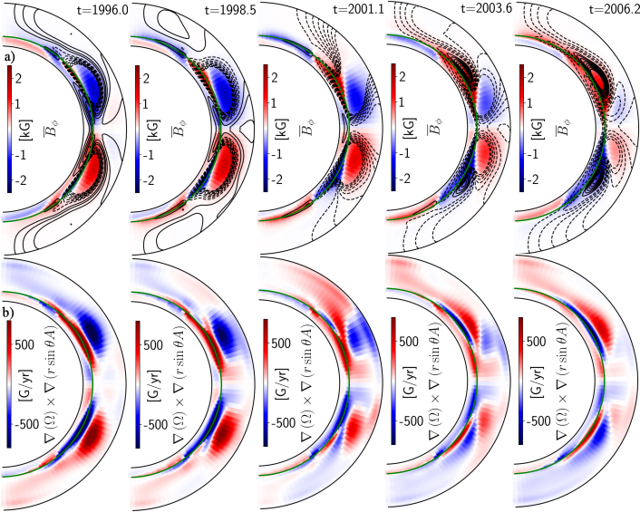
Figure 5 shows the axisymmetric toroidal magnetic field (images in the top panels), the poloidal magnetic field lines (the solid lines show the clockwise oriented field), and the corresponding toroidal field generation rate by the differential rotation, i.e., (bottom panels) in the convection zone in model S2 during Cycle 23. The toroidal field generation rate reaches its maximum of about 2 kG/yr at mid-latitudes near the bottom of the convection zone. These images and the accompanying animation illustrate the dynamo wave propagation and the induction effects of the radial and latitudinal gradients of the angular velocity on the evolving large-scale magnetic field. In the lower part of the convection zone, the radial gradient of the angular velocity stretches the closed parts of the axisymmetric poloidal magnetic field lines. This results in the opposite signs of the toroidal flux generation rate in the lower and upper parts of the convection zone. Simultaneously, it produces the dynamo wave propagating along the lines of constant rotation according to the Parker-Yoshimura rule (Parker, 1955; Yoshimura, 1975). The latitudinal shear stretches the open poloidal field lines in the upper half of the dynamo domain. The positive sign of the -effect in the Northern hemisphere results in a coordinated action of the radial and latitudinal shear in the upper part of the convection zone. It follows that the radial gradient of the solar differential rotation provides a substantial part of the toroidal flux inside the convection zone and affects the magnitude of the mean toroidal flux there. It is noteworthy that, similar to results presented in Fig.2 and Fig.4a effects of the differential rotation near the surface of the solar poles and near equator below the bottom of the convection zone have the same sign. The open poloidal flux and the latitudinal rotational shear control the magnitude of the subsequent cycle. Their properties affect the correlation of the polar magnetic field strength during the solar minima with the magnitude of the toroidal field dynamo wave of the subsequent magnetic cycle.
4 Discussion and Conclusions
The solar dynamo is responsible for the generation and decay of the axisymmetric toroidal and poloidal magnetic field fluxes on the Sun. Motivated by the results of Cameron & Schüssler (2015) (CS15), we analyzed the dynamo magnetic flux budget using solar synoptic observations and results of our mean-field dynamo models (Pipin et al., 2023). One of the hypotheses of CS15 is the dominant role of the surface latitudinal differential rotation in the generation of the axisymmetric toroidal magnetic field of the Sun. Our results suggest that the radial rotational shear can be important as well, at least for the mean-field type distributed dynamo models. The study shows the generation rate of the toroidal field by the differential rotation in the 3D dynamo models, which include the emergence of Bipolar Magnetic Regions (BMRs), is higher than in the corresponding axisymmetric 2D models without BMRs. This is because the BMRs activity provides the additional source of the poloidal magnetic field generation for this type of dynamo (P22).
We find that the toroidal flux generation rate by the surface latitudinal differential rotation strongly depends on the radial magnetic field profile in the polar regions. Observations show that the radial magnetic field is almost uniform near the solar poles during epochs of the solar minima. In contrast, the dynamo models show a sharp increase in the toroidal flux generation rate toward the poles. One reason could be a strong effect of the meridional circulation on the near-surface radial magnetic field. The toroidal flux generation rate by the latitudinal differential rotation reaches its maximum at the poles in the observations and dynamo models during the solar activity minima. This property explains the relative success of the correlation between the polar magnetic field strength and the magnitude of the subsequent magnetic cycle for the solar cycle predictions (e.g., Schatten et al., 1978; Choudhuri et al., 2007). Our results suggest that this correlation may depend on the profile of the radial magnetic field near solar poles. The long-term measurements of the large-scale solar magnetic fields in the solar polar regions can help to resolve the issue.
Acknowledgments
VP thanks the financial support of the Ministry of Science and Higher Education of the Russian Federation (Subsidy No.075-GZ/C3569/278). AK acknowledges the partial support of the NASA grants: NNX14AB70G, 80NSSC20K0602, 80NSSC20K1320, and 80NSSC22M0162.
Data Availability Statements. The data underlying this article are available by request.
References
- Abramenko et al. (2023) Abramenko, V. I., Suleymanova, R. A., & Zhukova, A. V. 2023, MNRAS, 518, 4746, doi: 10.1093/mnras/stac3338
- Babcock (1961) Babcock, H. W. 1961, ApJ, 133, 572, doi: 10.1086/147060
- Berger & Hornig (2018) Berger, M. A., & Hornig, G. 2018, Journal of Physics A Mathematical General, 51, 495501, doi: 10.1088/1751-8121/aaea88
- Brandenburg et al. (2023) Brandenburg, A., Elstner, D., Masada, Y., & Pipin, V. 2023, Space Sci. Rev., 219, 55, doi: 10.1007/s11214-023-00999-3
- Cameron & Schüssler (2015) Cameron, R., & Schüssler, M. 2015, Science, 347, 1333, doi: 10.1126/science.1261470
- Cameron & Schüssler (2023) —. 2023, arXiv e-prints, arXiv:2305.02253, doi: 10.48550/arXiv.2305.02253
- Choudhuri et al. (2007) Choudhuri, A. R., Chatterjee, P., & Jiang, J. 2007, Physical Review Letters, 98, 131103, doi: 10.1103/PhysRevLett.98.131103
- Getling et al. (2021) Getling, A. V., Kosovichev, A. G., & Zhao, J. 2021, ApJ, 908, L50, doi: 10.3847/2041-8213/abe45a
- Golovko (1998) Golovko, A. A. 1998, Astronomy Reports, 42, 546
- Guerrero et al. (2016) Guerrero, G., Smolarkiewicz, P. K., de Gouveia Dal Pino, E. M., Kosovichev, A. G., & Mansour, N. N. 2016, ApJ, 819, 104, doi: 10.3847/0004-637X/819/2/104
- Hazra et al. (2023) Hazra, G., Nandy, D., Kitchatinov, L., & Choudhuri, A. R. 2023, Space Sci. Rev., 219, 39, doi: 10.1007/s11214-023-00982-y
- Käpylä et al. (2016) Käpylä, M. J., Käpylä, P. J., Olspert, N., et al. 2016, A&A, 589, A56, doi: 10.1051/0004-6361/201527002
- Käpylä et al. (2022) Käpylä, M. J., Rheinhardt, M., & Brandenburg, A. 2022, ApJ, 932, 8, doi: 10.3847/1538-4357/ac5b78
- Kitchatinov & Pipin (1993) Kitchatinov, L. L., & Pipin, V. V. 1993, A&A, 274, 647
- Kitchatinov & Rüdiger (1992) Kitchatinov, L. L., & Rüdiger, G. 1992, A&A, 260, 494
- Kleeorin & Rogachevskii (1999) Kleeorin, N., & Rogachevskii, I. 1999, Phys. Rev.E, 59, 6724
- Kleeorin & Ruzmaikin (1982) Kleeorin, N. I., & Ruzmaikin, A. A. 1982, Magnetohydrodynamics, 18, 116
- Komm et al. (2018) Komm, R., Howe, R., & Hill, F. 2018, Sol. Phys., 293, 145, doi: 10.1007/s11207-018-1365-7
- Kosovichev & Pipin (2019) Kosovichev, A. G., & Pipin, V. V. 2019, ApJ, 871, L20, doi: 10.3847/2041-8213/aafe82
- Krause & Rädler (1980) Krause, F., & Rädler, K.-H. 1980, Mean-Field Magnetohydrodynamics and Dynamo Theory (Berlin: Akademie-Verlag), 271
- Leighton (1969) Leighton, R. B. 1969, ApJ, 156, 1, doi: 10.1086/149943
- Mitra et al. (2010) Mitra, D., Candelaresi, S., Chatterjee, P., Tavakol, R., & Brandenburg, A. 2010, Astronomische Nachrichten, 331, 130, doi: 10.1002/asna.200911308
- Moss & Brandenburg (1992) Moss, D., & Brandenburg, A. 1992, A&A, 256, 371
- Nagovitsyn et al. (2016) Nagovitsyn, Y. A., Tlatov, A. G., & Nagovitsyna, E. Y. 2016, Astronomy Reports, 60, 831, doi: 10.1134/S1063772916090055
- Norton et al. (2023) Norton, A., Howe, R., Upton, L., & Usoskin, I. 2023, Space Sci. Rev., 219, 64, doi: 10.1007/s11214-023-01008-3
- Obridko et al. (2023) Obridko, V. N., Shibalova, A. S., & Sokoloff, D. D. 2023, MNRAS, 523, 982, doi: 10.1093/mnras/stad1515
- Parker (1955) Parker, E. 1955, Astrophys. J., 122, 293
- Parker (1979) Parker, E. N. 1979, Cosmical magnetic fields: Their origin and their activity (Oxford: Clarendon Press)
- Paxton et al. (2013) Paxton, B., Cantiello, M., Arras, P., et al. 2013, ApJS, 208, 4, doi: 10.1088/0067-0049/208/1/4
- Pipin (2008) Pipin, V. V. 2008, Geophysical and Astrophysical Fluid Dynamics, 102, 21
- Pipin (2018) —. 2018, Journal of Atmospheric and Solar-Terrestrial Physics, 179, 185, doi: 10.1016/j.jastp.2018.07.010
- Pipin (2022) —. 2022, MNRAS, 514, 1522, doi: 10.1093/mnras/stac1434
- Pipin & Kosovichev (2011) Pipin, V. V., & Kosovichev, A. G. 2011, ApJL, 727, L45, doi: 10.1088/2041-8205/727/2/L45
- Pipin & Kosovichev (2019) —. 2019, ApJ, 887, 215, doi: 10.3847/1538-4357/ab5952
- Pipin & Kosovichev (2020) —. 2020, ApJ, 900, 26, doi: 10.3847/1538-4357/aba4ad
- Pipin et al. (2023) Pipin, V. V., Kosovichev, A. G., & Tomin, V. E. 2023, ApJ, 949, 7, doi: 10.3847/1538-4357/acaf69
- Rempel (2005) Rempel, M. 2005, ApJ, 631, 1286, doi: 10.1086/432610
- Ruediger & Brandenburg (1995) Ruediger, G., & Brandenburg, A. 1995, A&A, 296, 557
- Schaeffer (2013) Schaeffer, N. 2013, Geochemistry, Geophysics, Geosystems, 14, 751, doi: 10.1002/ggge.20071
- Schatten et al. (1978) Schatten, K. H., Scherrer, P. H., Svalgaard, L., & Wilcox, J. M. 1978, Geophys. Res. Lett., 5, 411, doi: 10.1029/GL005i005p00411
- Schrijver & Harvey (1984) Schrijver, C., & Harvey, K. 1984, Sol.Phys., 150, 1
- Schrijver & Harvey (1994) Schrijver, C. J., & Harvey, K. L. 1994, Sol. Phys., 150, 1, doi: 10.1007/BF00712873
- Schrinner (2011) Schrinner, M. 2011, A&A, 533, A108, doi: 10.1051/0004-6361/201116642
- Stenflo (1994) Stenflo, J. O. 1994, in NATO Advanced Study Institute (ASI) Series C, Vol. 433, Solar Surface Magnetism, ed. R. J. Rutten & C. J. Schrijver, 365
- Sun et al. (2011) Sun, X., Liu, Y., Hoeksema, J. T., Hayashi, K., & Zhao, X. 2011, Sol. Phys., 270, 9, doi: 10.1007/s11207-011-9751-4
- Warnecke et al. (2018) Warnecke, J., Rheinhardt, M., Tuomisto, S., et al. 2018, A&A, 609, A51, doi: 10.1051/0004-6361/201628136
- Warnecke et al. (2021) Warnecke, J., Rheinhardt, M., Viviani, M., et al. 2021, ApJ, 919, L13, doi: 10.3847/2041-8213/ac1db5
- Weber et al. (2023) Weber, M. A., Schunker, H., Jouve, L., & Işık, E. 2023, Space Sci. Rev., 219, 63, doi: 10.1007/s11214-023-01006-5
- Wilson et al. (1988) Wilson, P. R., Altrocki, R. C., Harvey, K. L., Martin, S. F., & Snodgrass, H. B. 1988, Nature, 333, 748, doi: 10.1038/333748a0
- Yoshimura (1975) Yoshimura, H. 1975, ApJ, 201, 740, doi: 10.1086/153940
5 Appendix
5.1 A. Data-Driven BMR Model
Injection of the bipolar magnetic regions is determined by
| (19) |
where the first term describes the -effect caused by the BMR tilt, and the second term models the magnetic buoyancy instability. The magnetic buoyancy velocity, , includes the turbulent and mean-field buoyancy effects (Kitchatinov & Rüdiger, 1992; Kitchatinov & Pipin, 1993; Ruediger & Brandenburg, 1995):
| (20) |
where, function , defines the location and formation of the unstable part of the magnetic field, the function describes effects of magnetic tension,
where, , ( for ) and subscript ’m’ marks unstable points. To determine the radial position of the unstable point, , we use the maximum of product . Here, we restrict to the upper part of the convection zone (above ), where reads,
| (21) |
where is the strength of the axisymmetric toroidal magnetic field and is the density profile. For the case of , we get Parker’s instability condition (Parker, 1979). In our model, we use . In the unstable region, we must have . We define as follows,
where is a kink-type function of radius,
| (23) | |||||
| (24) |
The latitudinal and longitudinal coordinates and in function are taken from the active region database. We relate the BMR areas to the parameter as follows,
where is the maximum observed area (in the millionth of the hemisphere) of the bipolar active regions. In our computations, we exclude BMRs with . The solar observations show a wide range of variations in the BMR emergence time, and growth rate, . Also, there are periods of simultaneous emergence of several BMRs in one hemisphere. To avoid the overlaps, we reformat the emergence initiation time as follows. Firstly, for such cases, we shift the emergence of subsequent BMRs by two time steps after the end of the previous BMR emergence. Secondly, we define the minimal emergence time days, (Weber et al., 2023), and assume that these BMRs have growth of day. Specifically, we define:
where is the total emergence time of the BMRs, is the growth rate. The parameters , and are taken from the NOAA database of solar active regions (https://www.swpc.noaa.gov/).
The -effect of the is given as follows
| (25) |
Here, we put the amplitude of the -effect to be determined by the local magnetic buoyancy velocity. The parameter controls the random fluctuation of the BMR tilt. The parameter, controls the mean amplitude of the BMR -effect and tilt. To reproduce Joe’s law, we put (PKT23). Note that, for , the BMRs are oriented along the axisymmetric toroidal field. We model the randomness of the tilt using the parameter . Similar to Rempel (2005), the evolution follows the equation,
| (26) | |||||
Here, is a Gaussian random number. It is renewed every time step, . The is the relaxation time of . . The parameters are introduced to get smooth variations of . Similarly to the above-cited papers, we choose the parameters of the Gaussian process as follows: , . We choose months, which is roughly equal to the lifetime of big active regions (Norton et al., 2023). The varies independently in the northern and southern hemispheres.
5.2 B. Dynamo model parameters
Figure 6 illustrates distributions of the angular velocity, meridional circulation, the - effect, and the eddy diffusivity in the nonmagnetic case model. The amplitude of the meridional circulation on the surface is about 13m/s. The angular velocity distribution is in agreement with the helioseismology data.

Figure 7(a) shows a snapshot of the radial magnetic field at the top of the dynamo domain for model S2 for the epoch of the solar maximum around the year 2000. Figure 7(b) shows the time-latitude diagram of the axisymmetric magnetic field in the model S2. Further details can be found inPKT23.
