Topology optimization of 3D flow fields for flow batteries
Abstract
As power generated from renewables becomes more readily available, the need for power-efficient energy storage devices, such as redox flow batteries, becomes critical for successful integration of renewables into the electrical grid. An important component in a redox flow battery is the planar flow field, which is usually composed of two-dimensional channels etched into a backing plate. As reactant-laden electrolyte flows into the flow battery, the channels in the flow field distribute the fluid throughout the reactive porous electrode. We utilize topology optimization to design flow fields with full three-dimensional geometry variation, i.e., 3D flow fields. Specifically, we focus on vanadium redox flow batteries and use the optimization algorithm to generate 3D flow fields evolved from standard interdigitated flow fields by minimizing the electrical and flow pressure power losses. To understand how these designs improve performance, we analyze the polarization of the reactant concentration and exchange current within the electrode to highlight how the designed flow fields mitigate the presence of electrode dead zones. While interdigitated flow fields can be heuristically engineered to yield high performance by tuning channel and land dimensions, such a process can be tedious; this work provides a framework for automating that design process.
-
February 2022
1 Introduction
The need for effective, large-scale energy storage continues to grow as the technology driving renewables continues to mature [1, 2, 3]. Renewable sources, such as wind and solar, are inherently weather and time dependent. Unfortunately, this intermittent energy supply is not always aligned with user needs for electricity, necessitating the use of power plants to meet peak demand [4, 5]. The mismatch between supply and demand hampers our ability to completely integrate renewables into the electrical grid. A stable, integrated electrical grid requires effective, large-scale energy storage – that is, efficient conversion from electrical energy to potential (e.g. chemical) energy, and vice versa – to buffer against this mismatch by storing and dispatching any excess generated electricity as necessary [6, 3]. Additionally, to be industrially relevant, these storage devices must operate with high power efficiency while remaining economically practical [7]. Redox flow batteries inherently decouple energy storage from power production, allowing the former to scale independently by merely increasing the size of the external storage vessels. As a result, redox flow batteries are an especially promising energy storage system to meet these needs [8, 9, 10, 11].
A critical problem in designing large-scale electrochemical systems, and energy storage systems such as redox flow batteries in particular, is the distribution of reactants to the electrode. The electrode is a porous media with a large exposed surface area of electrochemically active material [12]. Often, the electrode is made of a stochastic, graphitic or vitreous carbon material cohered into a bulk material such as a paper or felt [8]. Ideally, the electrolyte flow to the electrode will minimize excess power losses while appropriately distributing the reactant to promote reaction and mitigate the emergence of dead zones (i.e., low concentration regions with insufficient mass transfer) [13, 14, 15, 16, 17]. This problem is usually addressed by using sophisticated fluid distribution systems both external and internal to the electrochemical cell stack. The internal fluid distribution system is known as a flow field [14, 18], and significant effort has been devoted to understanding how the flow field architecture impacts device performance [19, 20, 21, 22, 23, 24, 25, 13].
Two of the most prevalently used flow field architectures are serpentine channel designs, where a single winding flow channel connects the electrolyte inlet to the outlet [26, 27, 28, 29, 30, 31, 32], and interdigitated channel designs, composed of a series of interlocking channels spanning the electrode [33, 34, 35, 36, 37]. A key difference between the two is that interdigitated flow fields force all of the electrolyte through the electrode while serpentine designs allow fluid bypass. Thus, for the latter, only a fraction of the flowing reactant penetrates the electrode [14]. Gerhardt et al. [33] investigated the interdigitated flow field both computationally and experimentally. They showed how losses due to fluid pumping and the electrical overpotential change with the widths of the fluid channels and solid lands. While the former is generally reduced with larger fluid channel width, the latter is generally reduced with larger solid land width. Furthermore, for their specific system, they identified channel and land widths that lead to a minimum in overall power loss, though these dimensions changed as the operating conditions were varied. While this, and related, work have elucidated many of the associated transport mechanisms, there remains much debate about choosing an optimal flow field geometry [38, 39]. This difficult question is exacerbated by the vast design space possible for each architecture, including the recognition that the optimal flow field could change depending on the chemistry employed, the operating conditions, and the scale, etc.
Indeed, recent work is now beginning to focus on more widely exploring this design space by studying flow fields which deviate from standard 2D (i.e., a geometry that only varies in two dimensions) interdigitated and serpentine configurations [40, 41, 42, 43]. This includes introducing hierarchy [41], splitting and reconfiguration [42], and also the inclusion of 3D features such as ramps and obstructions [43]. A central focus of these efforts is to increase performance at larger scales where standard flow field designs may be less effective [38, 41, 43].
Despite their novelty, these architectures remain predominantly two dimensional, driven in large part by manufacturing constraints. However, recent advances in additive and advanced manufacturing offer viable techniques for fabricating complex 3D parts for electrochemical systems including flow fields [44, 45, 46, 47, 48, 49]. Additively manufactured, porous electrodes which include 3D features have been demonstrated to lead to improved mass transfer at higher flow rates [50]. There is also evidence that introducing three-dimensional features into the flow field itself can provide high performance at industrially relevant scales, e.g., as demonstrated by the design of the flow field used in the Toyota Mirai, a fuel cell vehicle [51].
However, even as additive and advanced manufacturing technologies improve, the community lacks guidance on what 3D features to consider for these 3D flow fields, i.e., flow fields with significant geometry variation in all three dimensions. This difficulty can be attributed to the complex nature of the underlying physical phenomena that couples together simultaneous fluid transport, mass transfer, and electrostatics. While it would be possible to iterate on 3D designs using a combination of intuition and simulation, such a process would be tedious, computationally expensive, and slow. Instead, we propose to use topology optimization [52] to computationally guide flow field design. This method has seen significant advancements in recent years, and researchers have used topology optimization to aid in the design of heat exchangers [53, 54, 55, 56, 57, 58], structural supports [59, 60], and microfluidic devices [61, 62]. Additionally, topology optimization has been applied to the design of two-dimensional flow fields for both flow batteries [63, 64] and fuel cells [65]. More recently, Beck et al. [66] demonstrated the application of three-dimensional optimization to electrochemical transport, by designing an optimized and homogenized variable porosity electrode. Here, we leverage the ideas of that work, and develop a topology optimization method to design 3D flow fields.
In this work, we aim to use topology optimization, in tandem with a high-resolution electrochemical model of a redox flow battery, to design 3D flow fields. We specifically focus on the well-studied vanadium redox flow battery [67, 68, 69, 70, 71, 72], the most widely commercialized redox flow battery [7]. We seek to improve upon the popular interdigitated design, and in particular, we aim to showcase the pertinent three-dimensional features that arise. We perform the optimization to reduce the sum of electrical and fluid flow pumping power losses, and we identify how the qualitative design features of the optimized design change as the operating conditions of the flow battery change. We quantify the power efficiencies of the optimized designs, showcase how different optimal designs appear depending on the initial design provided to the optimization algorithm, and discuss how the optimized designs more evenly distribute reactant to the electrode. Since flow fields, and flow manifolds in general, are necessary for any engineered system requiring fluid and mass distribution, we also provide suggestions for how our work can be extended in the future.
2 Methods
Problem overview
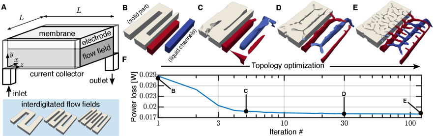
We consider the negative half-cell of a vanadium redox flow battery as shown in figure 1(A). Liquid electrolyte, comprised of a solution of and at a concentration in 1M sulfuric acid flows in, which is then guided by the flow field towards the porous carbon-felt electrode, where the reaction occurs on the surfaces of electrode fibers. The spent fluid then flows from the outlet. Inspired by the popularity and success of the interdigitated flow field design (examples of which are shown in the bottom of figure 1(A)), we utilize a combination of a continuum model of the flow battery half-cell following porous electrode theory [66, 73] – incorporating fluid mechanics, mass transfer, and electrostatics – and topology optimization to improve upon this design. An example of the optimization process used in this work is shown in figures 1(B-E). Specifically, the flow field designs at various iterations in the optimization process are shown, corresponding to points indicated on the plot of power loss plotted against iteration number in figure 1(F). To aid in visualization, in figures 1(B-E), half of the solid flow field is shown, and the negative of the solid part, i.e. the fluid channels within the flow field, are shown for the other half. In this work, we focus on a half-cell with experimentally relevant dimensions: the square porous carbon electrode has side length of cm, and thus an area of , and is thick, and the flow field is 3 mm thick.
We aim to design the flow field to minimize the excess power losses that occur for a specified discharge current and electrolyte flow rate . We consider in this work current densities and flow rates [71, 67, 33, 69, 72]. The total power loss is defined as
| (1) |
where is the half-cell overpotential, is the discharge current density, is the pump efficiency, which is assumed to be in this work, is the fluid pressure, and is the specified averaged inlet fluid velocity. The first term represents the electrical power loss due to the half-cell overpotential, while the second term represents the fluid pumping power loss. As highlighted by Gerhardt et al. [33], a flow field design with more solid present will typically have a reduced Ohmic electrical power loss due to the high conductivity of the solid, and a flow field design with more void will typically have a reduced fluid pumping power loss due to the reduced hydraulic resistance – this paradox highlights why optimization of this component is nontrivial. Equivalently, our goal is to maximize the overall power efficiency of the half-cell, which is defined as
| (2) |
where is the equilibrium half-cell potential. As defined, for a perfectly efficient cell and can be for a very poorly designed cell.
Continuum simulation
The equations governing the continuum electrochemical model are as follows. The fluid velocity is described by the steady incompressible Navier-Stokes equation with a Darcy drag,
| (3) | |||||
| (4) |
where is the fluid density, is the viscosity, is the pressure, and is the local permeability of the material. As described below, the topology optimization technique models the presence of solid and liquid material by smoothly varying the parameters using a position dependent design variable, . In the solid, takes on a large value to prevent fluid flow, in the liquid regions, , and in the fixed porous region representing the electrode, . This parameter thus controls the location of solid and liquid within the flow field and approximates the no-slip condition for the fluid velocity. At the inlet, we specify the velocity to be , and the fluid exits to zero pressure; no-slip is assumed at all other boundaries.
The mass transfer of the species concentration , where , is described by the steady advection-diffusion-reaction equation, given by,
| (5) |
where is the design variable dependent diffusivity, is the exposed surface area per volume of the porous electrode, and is an indicator function that returns in the electrode and elsewhere. The reaction within the homogenized electrode is given by , where is a mass transfer coefficient and is the concentration at the surface of the fibers of the electrode. At all boundaries, the no-flux condition is applied for .
The electrostatics of the solid and liquid are described by the following Poisson equations,
| (6) | |||||
| (7) |
where and are electric potentials of the liquid and solid, respectively, and and are the design variable dependent conductivities of the liquid and solid, respectively. The exchange current is given by the Butler-Volmer equation,
| (8) |
where is an arbitrary reference concentration to maintain dimensional consistency, is the local overpotential, , where is Faraday’s constant, is the ideal gas constant, is the temperature, and a charge transfer coefficient of has been assumed. The current is proportional to the mass transfer reaction term as . A current is discharged through the membrane via the liquid, so that at the membrane, and the current collector is attached to the solid part of the flow field so that at the current collector; all other boundaries are no-flux boundaries for the potential.
Topology optimization
We follow the optimization method described by Beck et al. [66], with some important differences. In contrast to [66], who performed optimization of a porous electrode via a homogenized model, we utilize topology optimization to generate flow field designs with well-defined solid and liquid boundaries separated by a thin, smoothly varying interface [52]. Our goal is to solve,
| (9) | |||||
| (10) |
where are the forward partial differential equations (PDEs) given in equations (3)-(7), and is the design variable within the flow field that is equal to where the flow field is pure liquid and equal to where the flow field is pure solid.
Within the flow field, the design variable is used to smoothly interpolate the material properties from that of pure solid to that of pure liquid. Thus, the permeability, diffusivities, and conductivities in equations (3)-(7) are all functions of the design variable. To ensure that optimized designs are “black-white,” i.e. comprised of pure solid and pure liquid with minimal material in between, the specific functional forms of the interpolations are chosen carefully (e.g. see [53]) and attain the appropriate values at the end points, and . These functions are described in the Supplementary Information.
To perform the optimization, the continuous adjoint approach is employed [74, 66]. Briefly, the Lagrangian of the problem is
| (11) |
The adjoint PDEs corresponding to each PDE given in equations (3)-(7) are derived analytically by setting the variation of with respect to each dependent variable to 0, i.e. . From this, the sensitivity is then determined by calculating . These equations are solved in OpenFOAM, and the sensitivities are used within the Method of Moving Asymptotes to update the values of in each computational cell [75]. For the simulations in this work, we use hexahedral meshes with M cells to solve the forward and adjoint PDEs. The Helmholtz filter with a filter radius of the mesh size used in the flow field, , is used to regularize the solution, and a Heaviside projection is used to push the solution to a black-white design [76]. This process is described in more detail in the Supplementary Information.
Estimation of electrochemical parameters
Estimated parameters and correlations used in our electrochemical simulation are shown in table 1. Notably, the Bruggeman correlation [71] is used to describe properties within the porous electrode. Specifically, in the electrode,
| (12) | |||||
| (13) | |||||
| (14) |
and in the flow field, interpolations relating the design variable to solid and liquid properties are described in the Supplementary Information.
-
Description Parameter Value Units Ref. Solid conductivity Est. Electrode porosity - [71] Electrode permeability [71] Electrode area/volume Est. Electrolyte conductivity Est. Electrolyte viscosity Est. Electrolyte density Est. Diffusivity [77] Mass transfer coeff. [78] Exchange current [71] Equilibrium potential [67]
3 Results and discussion
Optimized flow field designs
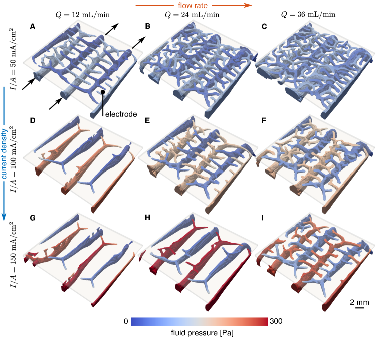
In figure 2, we show the liquid fraction of optimized flow fields for a range of operating conditions where the optimization is initialized with channel and land widths of 2 mm. In figures S1 and S2 of the Supplementary Information, results are also shown where the optimization is initialized with channel and land widths of 4 and 1.5 mm, respectively. The actual solid part is thus the negative of what is shown in the figure. The porous electrode is represented as a translucent sheet above the visible flow structures. As the operating current and flow rate change, the dominant physical phenomena change. This, in turn, changes the ratio of electrical power losses to pressure power losses, leading to qualitatively different optimal flow field designs. When the flow rate is low, the optimized fluid channels are thin and the flow field is comprised mostly of solid material, suggesting that an interdigitated design with thin channels would perform well. At even lower flow rates, we observe no clear three-dimensional structures that form in the nearly fully-solid flow field, and these designs are shown in figure S3 of the Supplementary Information. In contrast, as the flow rate increases and more reactant is supplied to the electrode, smaller secondary channels emerge from the primary fluid channels beneath – resembling a tree-root structure – and guide fluid up into the electrode. Additionally, the larger primary fluid distribution channels grow larger, presumably to avoid large fluid resistances and increased flow power losses.
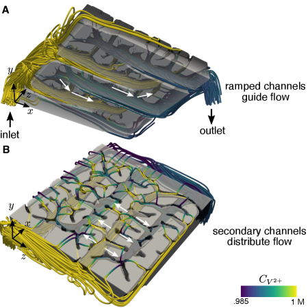
The observed features of the optimized designs are fully three-dimensional, providing evidence that there is room for improvement in more popular two-dimensional designs. Remarkably, the optimization algorithm automatically identified features which have previously been devised through experimentation. At flow rates of 12 mL/min and 24 mL/min, the optimized designs show a ramped channel design as in the work of Akuzum et al. [43], helping to guide both unreacted reactant up into the electrode and used reactant down out of the electrode. The optimized design, however, does further taper the channel in addition to ramping. Additionally, at high flow rates and currents, the optimization algorithm not only re-identified the use of hierarchy, but it further suggests that the density of branching should increase at lower operating currents and higher flow rates [41]. The optimization procedure not only suggests interesting design candidates, but because it uses a model and simulation for the system behavior to determine the geometries, it also provides strategies to most effectively employ the 3D features. To provide further intuition on the design features that form and how fluid flows through the solid part, in figure 3, we show a visualization of the fluid streamlines through the flow field for the example case where and . These streamlines are colored by reactant concentration to highlight the depletion of concentration as fluid leaves the flow field. In figure 3(A), we observe the previously described ramps that appear at the ends of the primary fluid distribution channels, and in figure 3(B), we observe the smaller secondary channels that form at the flow field-electrode interface that work to evenly distribute fluid across the electrode.
In our optimization procedure, it is important to note that the length scale of the smallest feature size can, in principle, be controlled to meet minimum feature size constraints imposed by a specific additive manufacturing technique. As described in §2, in these optimization simulations, a Helmholtz filter [76] is used to regularize the flow field design, which as a result sets the minimum feature size that can arise here. In this work, we have chosen a filter radius that results in a minimum feature size of approximately mm, however, this filter radius could be modified. Current additive manufacturing techniques have resolutions that range from sub-micron to millimeter scale [44].
Power losses and efficiencies
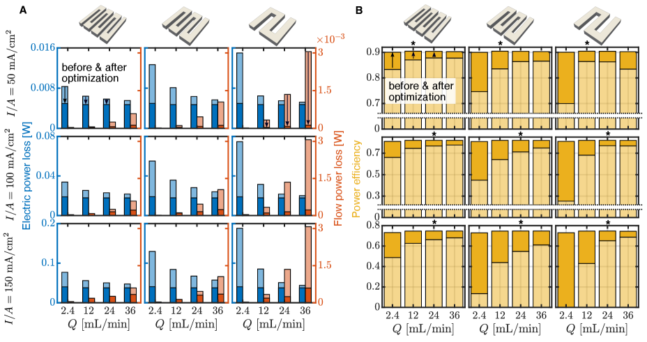
The qualitative design features observed in figure 2 are now quantitatively supported. As implied by the variety of designs shown in figure 2, the optimal flow field design is achieved by balancing the electrical and flow power losses. This balance is similar to what is observed in the optimized homogenized porous electrodes studied by Beck et al. [66], where lower operating flow rates lead to less porous optimized structures and vice versa. The associated electric and flow power losses of the optimized designs are shown in figure 4(A), along with the power losses obtained with the traditional, unoptimized interdigitated flow field. The power efficiencies , calculated from equation (2), corresponding to these power losses are shown in figure 4(B). In all cases, the optimized designs lead to greater power efficiency than the interdigitated designs.
At a particular current, traditional flow field designs yield power losses where the electric losses are maximized when the supplied flow rate is minimized, and the flow losses are maximized when the supplied flow rate is maximized. Thus, the optimization prioritizes reduction of the appropriate power loss contribution based on the operating conditions. This is evident in figure 4(A) from the large reduction in the electric power loss for designs generated for low flow rates, and, conversely, in the large reduction in flow power loss for designs generated for high flow rates. For the particular system studied here, the electrical power losses typically dominate, with the flow power losses typically contributing , due to the fact that the dominant source of flow resistance is only associated with the thin porous electrode. For larger area electrodes, the flow losses would be larger, and this optimization process would appropriately reprioritize the loss reduction. Since the specific choice of channel and land widths of traditional interdigitated flow fields are known to affect performance, we also consider simulations initialized with channel and land widths of 1.5 and 4 mm, and observe the same trends for each initial condition.
For a given current, the power efficiency of the optimized design reaches approximately the same value across all of the flow rates and initial conditions tested. For example, when , the optimized power efficiency is always . In contrast, at the same current density, the standard interdigitated designs have efficiency , when and the channel and land widths are 4mm, while , when and the channel and land widths are 1.5 mm. The improvement from optimization at this current density thus ranges from . This demonstrates that topology optimization can be an effective tool to identify a high performance geometry regardless of the desired operating conditions. Alternatively, a single standard unoptimized design shows strong variations in performance across operating conditions. While it is certainly possible to use a traditional interdigitated design to yield high performance, a significant amount of testing is required to find the optimal fluid channel and solid land widths for the specific system used; this process needs to be repeated whenever these conditions change. For example, Gerhardt et al. [33] find a channel and land width that yields a maximum pumping-corrected voltage efficiency, a metric similar to our definition of , of for their ferrocyanide-ferricyanide flow battery system operating at , but also discuss how the optimal dimensions change as the operating conditions change. A key takeaway from the present work is that this iterative process can be automated through the use of topology optimization methods such as the one presented here.
Analysis of 3D flow field design features
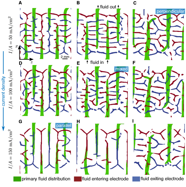
All of the flow field designs presented in figure 2 have been obtained by conducting simulations with the same initial condition: an interdigitated flow field with channel and land width of . However, as evidenced by the power efficiencies presented in figure 4(B), the optimization scheme is able to yield a design with similar performance, regardless of the initial channel and land widths chosen, even though the ultimate design depends on the specific initial conditions. To further understand how the optimization procedure is selecting design features, in figure 5, we show slices of the fluid fraction of the optimized flow fields from figures 2, S1, and S2, where the flow rate is selected based on the optimal power efficiency as observed in figure 4(B). In doing so, we highlight how the optimized three-dimensional structures change for various currents and starting initial conditions. In green, the primary underlying fluid distribution channels are shown by plotting the fluid fraction along a slice within the flow field ( mm), and in blue and red, the secondary fluid channels are shown by plotting the fluid fraction along a slice near the flow field-electrode interface ( mm). The fresh reactant-laden fluid thus enters the flow field through the green channels on the bottom, enters the electrode in the out-of-page direction through the red high pressure regions, exits the electrode through the blue low pressure regions, and out of the device through the green channels on the top.
The structure of the secondary channels that form provide clues for what constitutes an optimal design. In figure 5(C), where the current is relatively low and the initial interdigitated design has relatively thick channel and land widths, secondary channels appear perpendicular to the primary flow channels. In contrast, in figure 5(G), where the opposite is true, secondary channels appear parallel and coincident to the primary flow channels. In other cases, a mixed regime appears, where both parallel and perpendicular secondary channels appear. This provides evidence that the initial channel and land widths in figure 5(C) are too thick for the system, and the optimization algorithm works to create secondary channels to more evenly distribute reactant. Similarly, this shows that the initial channel and land widths in figure 5(G) are close to optimal, and the interdigitated design under these operating conditions already performs relatively well. In figure 5(A), we observe a design resembling that of figure 5(G), but with small perpendicular channels appearing: since the operating current in this case is lower, there is less need for the optimization to prioritize electrical contact with the flow field.
To further understand and quantify how evenly the reactant is distributed, we consider the dimensionless root-mean-squared-deviation of the oxidant concentration within the electrode,
| (15) |
where denotes an average over the volume of the porous electrode. This quantity thus gives a measure of the concentration polarization within the electrode. Similarly, we also consider the dimensionless root-mean-squared-deviation of the exchange current within the electrode,
| (16) |
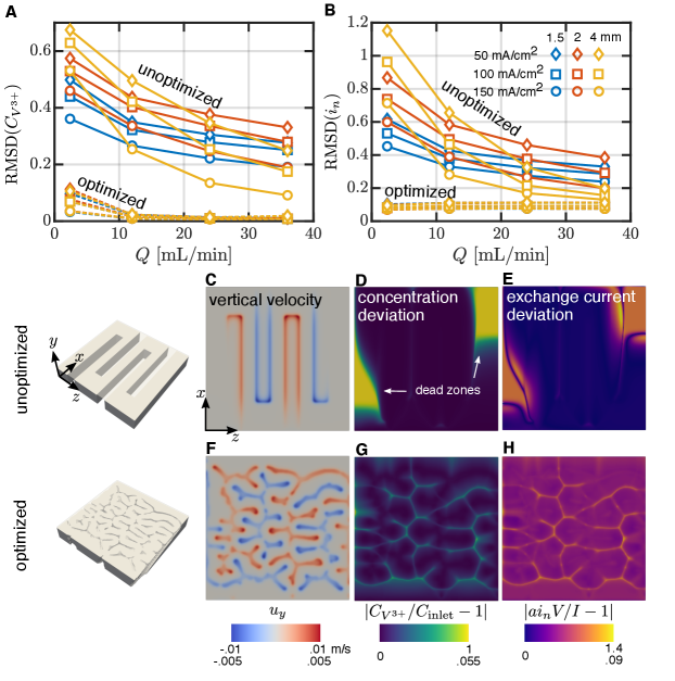
where is the exposed surface area per volume of the electrode, is the electrode volume, and is the exchange current given by the Butler-Volmer relation in equation (8). It is evident that the lower these quantities are, the more uniform the distribution of reactant and Faradaic reaction. In the limit of perfect uniformity, both approach a value of zero. In figure 6(A) and (B), we show both and as a function of flow rate for various currents and initial channel and land widths. In all cases, we observe an appreciable reduction in these quantities for the optimized designs, with the most significant improvement observed at low flow rate.
While both of these quantities give a global measure of how well the reactant is distributed within the electrode, it is also insightful to examine the local quantities. In figure 6(C)-(H), we compare the vertical fluid velocity, local concentration polarization, and local exchange current deviation within a slice of the electrode between the unoptimized and optimized flow field; we consider the particular case where , , and the initial channel and land width is . This highlights how the optimized design is able to more evenly utilize the entire electrode and avoid electrode dead zones. In figure 6(C), we observe that there is a large area of the electrode where the fluid is essentially stagnant. In contrast, the optimized design is able to deliver fluid to and from the electrode nearly uniformly (figure 6(F)), thus reducing the concentration and exchange current polarization (figure 6(G,H)).
4 Conclusions
In this work, we have shown that topology optimization, coupled with a model of the fluid mechanics, mass transfer, and electrostatics describing a flow battery, can be used to improve the performance of a flow field. Specifically, we use topology optimization to design flow fields with full three-dimensional variation, i.e. 3D flow fields. We have improved upon the popular two-dimensional interdigitated flow field design and identified pertinent three-dimensional features, such as ramps and hierarchy, that have previously been devised heuristically. Additionally, we have shown that our optimized designs lead to better overall reactant and reaction distribution within the electrode. Notably, while using a traditional interdigitated design can certainly yield high performance, this requires tedious testing to find the optimal land and channel widths for the particular system; our method has the potential to automate that process. Understanding and improving fluid and mass distribution in electrochemical systems such as flow batteries is critical, and this work gives preliminary evidence that investing effort into developing advanced manufacturing techniques to fabricate such complex components may be fruitful. Our ongoing work includes experimentally demonstrating that the flow fields like the ones described in the present work can provide real-world benefit.
There are a number of other considerations that may need to be taken into account in an industrial setting for a specific application. For example, one may be interested in maximizing the single-pass conversion efficiency of the reactant, instead of the power loss, when considering a system-level analysis of a flow battery stack. Next, while we have focused on a particular flow battery size in this work, it would be of interest to explore how the benefits of optimization are affected as the device is scaled up. Certainly, the ratio of electrical losses to flow losses would be expected to change with system size. Furthermore, it would be of interest to understand how the optimized flow fields in this work perform within a full cell, where the membrane would be expected to make a nontrivial contribution to the performance. In a real-world application, it would also be important to understand whether or not these optimized designs would perform well in the presence of obstacles such as bubbles or unwanted debris that can clog flow channels. Finally, while flow batteries have been subject of the present work, the distribution of reactants remains to be a key problem in a range of engineered systems, such as [79] and water electrolyzers, fuel cells, and bioreactors. Given a particular system chemistry and desired quantity to be minimized, the process outlined in this work can be repeated, leading to the potential to improve mass distribution in such systems.
References
References
- [1] Steven Chu and Arun Majumdar. Opportunities and challenges for a sustainable energy future. nature, 488(7411):294–303, 2012.
- [2] Steven Chu, Yi Cui, and Nian Liu. The path towards sustainable energy. Nature materials, 16(1):16–22, 2017.
- [3] Turgut M Gür. Review of electrical energy storage technologies, materials and systems: challenges and prospects for large-scale grid storage. Energy Environ. Sci., 11(10):2696–2767, 2018.
- [4] Anya Castillo and Dennice F Gayme. Grid-scale energy storage applications in renewable energy integration: A survey. Energy Conversion and Management, 87:885–894, 2014.
- [5] Erik Ela, Michael Milligan, and Brendan Kirby. Operating reserves and variable generation. Technical report, National Renewable Energy Lab.(NREL), Golden, CO (United States), 2011.
- [6] Haisheng Chen, Thang Ngoc Cong, Wei Yang, Chunqing Tan, Yongliang Li, and Yulong Ding. Progress in electrical energy storage system: A critical review. Progress in natural science, 19(3):291–312, 2009.
- [7] Gareth Kear, Akeel A Shah, and Frank C Walsh. Development of the all-vanadium redox flow battery for energy storage: a review of technological, financial and policy aspects. International journal of energy research, 36(11):1105–1120, 2012.
- [8] Adam Z Weber, Matthew M Mench, Jeremy P Meyers, Philip N Ross, Jeffrey T Gostick, and Qinghua Liu. Redox flow batteries: a review. Journal of applied electrochemistry, 41(10):1137–1164, 2011.
- [9] Grigorii L Soloveichik. Flow batteries: current status and trends. Chemical reviews, 115(20):11533–11558, 2015.
- [10] Wei Wang, Qingtao Luo, Bin Li, Xiaoliang Wei, Liyu Li, and Zhenguo Yang. Recent progress in redox flow battery research and development. Advanced Functional Materials, 23(8):970–986, 2013.
- [11] Mike L Perry and Adam Z Weber. Advanced redox-flow batteries: a perspective. Journal of The Electrochemical Society, 163(1):A5064, 2015.
- [12] Gang Qiu, Abhijit S Joshi, CR Dennison, KW Knehr, EC Kumbur, and Ying Sun. 3-d pore-scale resolved model for coupled species/charge/fluid transport in a vanadium redox flow battery. Electrochimica Acta, 64:46–64, 2012.
- [13] E Knudsen, P Albertus, KT Cho, AZ Weber, and A Kojic. Flow simulation and analysis of high-power flow batteries. Journal of Power Sources, 299:617–628, 2015.
- [14] Xinyou Ke, Joseph M Prahl, J Iwan D Alexander, Jesse S Wainright, Thomas A Zawodzinski, and Robert F Savinell. Rechargeable redox flow batteries: flow fields, stacks and design considerations. Chemical Society Reviews, 47(23):8721–8743, 2018.
- [15] V Pavan Nemani and Kyle C Smith. Uncovering the role of flow rate in redox-active polymer flow batteries: simulation of reaction distributions with simultaneous mixing in tanks. Electrochimica Acta, 247:475–485, 2017.
- [16] Purna C Ghimire, Arjun Bhattarai, Rüdiger Schweiss, Günther G Scherer, Nyunt Wai, and Qingyu Yan. A comprehensive study of electrode compression effects in all vanadium redox flow batteries including locally resolved measurements. Applied Energy, 230:974–982, 2018.
- [17] Andrew A Wong, Shmuel M Rubinstein, and Michael J Aziz. Direct visualization of electrochemical reactions and heterogeneous transport within porous electrodes in operando by fluorescence microscopy. Cell Reports Physical Science, 2(4):100388, 2021.
- [18] Luis F Arenas, Carlos Ponce de León, and Frank C Walsh. Redox flow batteries for energy storage: their promise, achievements and challenges. Current Opinion in Electrochemistry, 16:117–126, 2019.
- [19] S Kumar and S Jayanti. Effect of flow field on the performance of an all-vanadium redox flow battery. Journal of Power Sources, 307:782–787, 2016.
- [20] Mirko Messaggi, Patrizio Canzi, R Mereu, A Baricci, F Inzoli, A Casalegno, and M Zago. Analysis of flow field design on vanadium redox flow battery performance: Development of 3d computational fluid dynamic model and experimental validation. Applied energy, 228:1057–1070, 2018.
- [21] Sandip Maurya, Phong Thanh Nguyen, Yu Seung Kim, Qinjun Kang, and Rangachary Mukundan. Effect of flow field geometry on operating current density, capacity and performance of vanadium redox flow battery. Journal of Power Sources, 404:20–27, 2018.
- [22] T Jyothi Latha and S Jayanti. Hydrodynamic analysis of flow fields for redox flow battery applications. Journal of Applied Electrochemistry, 44(9):995–1006, 2014.
- [23] Jacob Houser, Jason Clement, Alan Pezeshki, and Matthew M Mench. Influence of architecture and material properties on vanadium redox flow battery performance. Journal of Power Sources, 302:369–377, 2016.
- [24] Robert M Darling and Mike L Perry. The influence of electrode and channel configurations on flow battery performance. Journal of The Electrochemical Society, 161(9):A1381, 2014.
- [25] Xianguo Li and Imran Sabir. Review of bipolar plates in pem fuel cells: Flow-field designs. International journal of hydrogen energy, 30(4):359–371, 2005.
- [26] Qian Xu, TS Zhao, and Cheng Zhang. Performance of a vanadium redox flow battery with and without flow fields. Electrochimica Acta, 142:61–67, 2014.
- [27] Ravendra Gundlapalli and Sreenivas Jayanti. Effect of channel dimensions of serpentine flow fields on the performance of a vanadium redox flow battery. Journal of Energy Storage, 23:148–158, 2019.
- [28] Qian Xu, TS Zhao, and PK Leung. Numerical investigations of flow field designs for vanadium redox flow batteries. Applied energy, 105:47–56, 2013.
- [29] Xinyou Ke, J Iwan D Alexander, Joseph M Prahl, and Robert F Savinell. Flow distribution and maximum current density studies in redox flow batteries with a single passage of the serpentine flow channel. Journal of Power Sources, 270:646–657, 2014.
- [30] Xinyou Ke, J Iwan D Alexander, Joseph M Prahl, and Robert F Savinell. A simple analytical model of coupled single flow channel over porous electrode in vanadium redox flow battery with serpentine flow channel. Journal of Power Sources, 288:308–313, 2015.
- [31] Xinyou Ke, Joseph M Prahl, J Iwan D Alexander, and Robert F Savinell. Redox flow batteries with serpentine flow fields: Distributions of electrolyte flow reactant penetration into the porous carbon electrodes and effects on performance. Journal of Power Sources, 384:295–302, 2018.
- [32] Xinyou Ke, Joseph M Prahl, J Iwan D Alexander, and Robert F Savinell. Mathematical modeling of electrolyte flow in a segment of flow channel over porous electrode layered system in vanadium flow battery with flow field design. Electrochimica Acta, 223:124–134, 2017.
- [33] Michael R Gerhardt, Andrew A Wong, and Michael J Aziz. The effect of interdigitated channel and land dimensions on flow cell performance. Journal of The Electrochemical Society, 165(11):A2625, 2018.
- [34] Cong Yin, Yan Gao, Shaoyun Guo, and Hao Tang. A coupled three dimensional model of vanadium redox flow battery for flow field designs. Energy, 74:886–895, 2014.
- [35] Shohji Tsushima and Takahiro Suzuki. Modeling and simulation of vanadium redox flow battery with interdigitated flow field for optimizing electrode architecture. Journal of The Electrochemical Society, 167(2):020553, 2020.
- [36] Cong Yin, Yan Gao, Guangyou Xie, Ting Li, and Hao Tang. Three dimensional multi-physical modeling study of interdigitated flow field in porous electrode for vanadium redox flow battery. Journal of Power Sources, 438:227023, 2019.
- [37] Ravendra Gundlapalli and Sreenivas Jayanti. Performance characteristics of several variants of interdigitated flow fields for flow battery applications. Journal of Power Sources, 467:228225, 2020.
- [38] Xinyou Ke, Joseph M Prahl, J. Iwan D Alexander, Jesse S Wainright, Thomas A Zawodzinski, and Robert F Savinell. Rechargeable redox flow batteries: flow fields, stacks and design considerations. Chem. Soc. Rev., 47(23):8721–8743, 2018.
- [39] Oladapo Christopher Esan, Xingyi Shi, Zhefei Pan, Xiaoyu Huo, Liang An, and T S Zhao. Modeling and Simulation of Flow Batteries. Adv. Energy Mater., 22:2000758–42, June 2020.
- [40] Kleber Marques Lisboa, Julian Marschewski, Neil Ebejer, Patrick Ruch, Renato Machado Cotta, Bruno Michel, and Dimos Poulikakos. Mass transport enhancement in redox flow batteries with corrugated fluidic networks. Journal of Power Sources, 359:322–331, 2017.
- [41] Yikai Zeng, Fenghao Li, Fei Lu, Xuelong Zhou, Yanping Yuan, Xiaoling Cao, and Bo Xiang. A hierarchical interdigitated flow field design for scale-up of high-performance redox flow batteries. Applied Energy, 238:435–441, 2019.
- [42] Ravendra Gundlapalli and Sreenivas Jayanti. Effective splitting of serpentine flow field for applications in large-scale flow batteries. Journal of Power Sources, 487:229409, 2021.
- [43] Bilen Akuzum, Yigit Can Alparslan, Nicholas C Robinson, Ertan Agar, and E Caglan Kumbur. Obstructed flow field designs for improved performance in vanadium redox flow batteries. Journal of Applied Electrochemistry, 49(6):551–561, 2019.
- [44] Adriano Ambrosi, Raymond Rong Sheng Shi, and Richard D Webster. 3d-printing for electrolytic processes and electrochemical flow systems. Journal of Materials Chemistry A, 8(42):21902–21929, 2020.
- [45] Greig Chisholm, Philip J Kitson, Niall D Kirkaldy, Leanne G Bloor, and Leroy Cronin. 3d printed flow plates for the electrolysis of water: an economic and adaptable approach to device manufacture. Energy & Environmental Science, 7(9):3026–3032, 2014.
- [46] Jesse R Hudkins, Danika G Wheeler, Bruno Peña, and Curtis P Berlinguette. Rapid prototyping of electrolyzer flow field plates. Energy & Environmental Science, 9(11):3417–3423, 2016.
- [47] Gaoqiang Yang, Jingke Mo, Zhenye Kang, Yeshi Dohrmann, Frederick A List III, Johney B Green Jr, Sudarsanam S Babu, and Feng-Yuan Zhang. Fully printed and integrated electrolyzer cells with additive manufacturing for high-efficiency water splitting. Applied Energy, 215:202–210, 2018.
- [48] Gaoqiang Yang, Shule Yu, Jingke Mo, Zhenye Kang, Yeshi Dohrmann, Frederick A List III, Johney B Green Jr, Sudarsanam S Babu, and Feng-Yuan Zhang. Bipolar plate development with additive manufacturing and protective coating for durable and high-efficiency hydrogen production. Journal of Power Sources, 396:590–598, 2018.
- [49] Justin C Bui, Jonathan T Davis, and Daniel V Esposito. 3d-printed electrodes for membraneless water electrolysis. Sustainable Energy & Fuels, 4(1):213–225, 2020.
- [50] Victor A Beck, Anna N Ivanovskaya, Swetha Chandrasekaran, Jean-Baptiste Forien, Sarah E Baker, Eric B Duoss, and Marcus A Worsley. Inertially enhanced mass transport using 3d-printed porous flow-through electrodes with periodic lattice structures. Proceedings of the National Academy of Sciences, 118(32), 2021.
- [51] Toshihiko Yoshida and Koichi Kojima. Toyota mirai fuel cell vehicle and progress toward a future hydrogen society. The Electrochemical Society Interface, 24(2):45, 2015.
- [52] Ole Sigmund and Kurt Maute. Topology optimization approaches. Structural and Multidisciplinary Optimization, 48(6):1031–1055, 2013.
- [53] Sumer B Dilgen, Cetin B Dilgen, David R Fuhrman, Ole Sigmund, and Boyan S Lazarov. Density based topology optimization of turbulent flow heat transfer systems. Structural and Multidisciplinary Optimization, 57(5):1905–1918, 2018.
- [54] Hiroki Kobayashi, Kentaro Yaji, Shintaro Yamasaki, and Kikuo Fujita. Freeform winglet design of fin-and-tube heat exchangers guided by topology optimization. Applied Thermal Engineering, 161:114020, 2019.
- [55] Lukas Christian Høghøj, Daniel Ruberg Nørhave, Joe Alexandersen, Ole Sigmund, and Casper Schousboe Andreasen. Topology optimization of two fluid heat exchangers. International Journal of Heat and Mass Transfer, 163:120543, 2020.
- [56] Florian Feppon, Grégoire Allaire, Charles Dapogny, and Pierre Jolivet. Body-fitted topology optimization of 2d and 3d fluid-to-fluid heat exchangers. Computer Methods in Applied Mechanics and Engineering, 376:113638, 2021.
- [57] Miguel A Salazar De Troya, Daniel A Tortorelli, and Victor A Beck. Two dimensional topology optimization of heat exchangers with the density and level-set methods. In 14th WCCM-ECCOMAS Congress, volume 1300. Lawrence Livermore National Lab.(LLNL), Livermore, CA (United States), 2021.
- [58] Miguel A Salazar de Troya, Daniel A Tortorelli, Julian Andrej, and Victor A Beck. Three-dimensional topology optimization of heat exchangers with the level-set method. arXiv preprint arXiv:2111.09471, 2021.
- [59] Martin P Bendsøe. Optimal shape design as a material distribution problem. Structural optimization, 1(4):193–202, 1989.
- [60] Tyler E Bruns and Daniel A Tortorelli. Topology optimization of non-linear elastic structures and compliant mechanisms. Computer methods in applied mechanics and engineering, 190(26-27):3443–3459, 2001.
- [61] Allan Gersborg-Hansen, Ole Sigmund, and Robert B Haber. Topology optimization of channel flow problems. Structural and multidisciplinary optimization, 30(3):181–192, 2005.
- [62] Thomas Borrvall and Joakim Petersson. Topology optimization of fluids in stokes flow. International journal for numerical methods in fluids, 41(1):77–107, 2003.
- [63] Kentaro Yaji, Shintaro Yamasaki, Shohji Tsushima, Takahiro Suzuki, and Kikuo Fujita. Topology optimization for the design of flow fields in a redox flow battery. Structural and multidisciplinary optimization, 57(2):535–546, 2018.
- [64] Chih-Hsiang Chen, Kentaro Yaji, Shintaro Yamasaki, Shohji Tsushima, and Kikuo Fujita. Computational design of flow fields for vanadium redox flow batteries via topology optimization. Journal of Energy Storage, 26:100990, 2019.
- [65] Reza Behrou, Alberto Pizzolato, and Antoni Forner-Cuenca. Topology optimization as a powerful tool to design advanced pemfcs flow fields. International Journal of Heat and Mass Transfer, 135:72–92, 2019.
- [66] Victor A Beck, Jonathan J Wong, Charles F Jekel, Daniel A Tortorelli, Sarah E Baker, Eric B Duoss, and Marcus A Worsley. Computational design of microarchitected porous electrodes for redox flow batteries. Journal of Power Sources, 512:230453, 2021.
- [67] Liyu Li, Soowhan Kim, Wei Wang, M Vijayakumar, Zimin Nie, Baowei Chen, Jianlu Zhang, Guanguang Xia, Jianzhi Hu, Gordon Graff, et al. A stable vanadium redox-flow battery with high energy density for large-scale energy storage. Advanced Energy Materials, 1(3):394–400, 2011.
- [68] Qiong Zheng, Xianfeng Li, Yuanhui Cheng, Guiling Ning, Feng Xing, and Huamin Zhang. Development and perspective in vanadium flow battery modeling. Applied energy, 132:254–266, 2014.
- [69] Trevor J Davies and Joseph J Tummino. High-performance vanadium redox flow batteries with graphite felt electrodes. C, 4(1):8, 2018.
- [70] Yun Wang and Sung Chan Cho. Analysis and three-dimensional modeling of vanadium flow batteries. Journal of The Electrochemical Society, 161(9):A1200, 2014.
- [71] AA Shah, MJ Watt-Smith, and FC Walsh. A dynamic performance model for redox-flow batteries involving soluble species. Electrochimica Acta, 53(27):8087–8100, 2008.
- [72] Xiangkun Ma, Huamin Zhang, and Feng Xing. A three-dimensional model for negative half cell of the vanadium redox flow battery. Electrochimica Acta, 58:238–246, 2011.
- [73] John Newman and William Tiedemann. Porous-electrode theory with battery applications. AIChE Journal, 21(1):25–41, 1975.
- [74] Carsten Othmer. A continuous adjoint formulation for the computation of topological and surface sensitivities of ducted flows. International journal for numerical methods in fluids, 58(8):861–877, 2008.
- [75] K Svandberg. The method of moving asymptotes - a new method for structural optimization. International Journal for Numerical Methods in Engineering, 24:359–373, 1987.
- [76] Boyan Stefanov Lazarov and Ole Sigmund. Filters in topology optimization based on helmholtz-type differential equations. International Journal for Numerical Methods in Engineering, 86(6):765–781, 2011.
- [77] Tomoo Yamamura, Nobutaka Watanabe, Takashi Yano, and Yoshinobu Shiokawa. Electron-transfer kinetics of np3+/ np4+, npo2+/ npo2 2+, v2+/ v3+, and vo2+/ vo2+ at carbon electrodes. Journal of The Electrochemical Society, 152(4):A830, 2005.
- [78] D Schmal, J Van Erkel, and PJ Van Duin. Mass transfer at carbon fibre electrodes. Journal of applied electrochemistry, 16(3):422–430, 1986.
- [79] Danika G Wheeler, Benjamin AW Mowbray, Angelica Reyes, Faezeh Habibzadeh, Jingfu He, and Curtis P Berlinguette. Quantification of water transport in a co 2 electrolyzer. Energy & Environmental Science, 13(12):5126–5134, 2020.