Topology optimization enhances the distinguishability and reconstructability of electrical resistance tomography based sensors
Abstract
In the majority of applications of electrical resistance tomography (ERT) the estimation problem consists of either the estimation of spatial conductivity change over an existing background or the estimation of spatial distribution of conductivity of the entire target, including the background. In some instances however, it is possible to design the background conductivity; an example of such application is the design of ERT-based sensors where the background conductivity can be engineered. In such applications the natural question is whether the background conductivity can be engineered in such a way to increase the distinguishability and further reconstructability of the sensor. The present paper, uses topology optimization to design the background conductivity to achieve optimal distinguishability. Then, ERT reconstructions suggest the enhancements of reconstructability using topology optimized sensor.
Keywords: Complete Electrode Model (CEM), Constrained Optimization, Electrical Imaging, Electrical Resistance Tomography (ERT), Inverse Problems, Topology Optimization.
1 Introduction
Electrical Resistance Tomography (ERT) is an imaging modality in which the spatial distribution of electrical conductivity (or resistivity) of a target is reconstructed based on a set of electric current injections and their corresponding measured potentials [1]. For this purpose, typically electrodes are installed at the boundary of a target; the same set of electrodes are used for current injections and potential measurements.
ERT has many medical and industrial applications. In the majority of these applications, the goal is to estimate the change of conductivity over an existing background [2, 3, 4, 5, 6, 7], to estimate the spatial distribution of conductivity of the entire target including the background[8, 2, 9, 10, 11], or simultaneously estimate a change and the background spatial conductivity distribution [12, 13]. In these applications the background conductivity may be unknown, non-uniform, or otherwise. In some instances however, there is a possibility of designing the background conductivity to achieve a certain objective. An example of such application is the so-called ERT-based sensing skin (referred to as sensing skin hereafter)[10, 11, 5, 6, 7].
Sensing skin is a thin layer of electrically conductive materials that is applied to the surface of a structure in the form of paint or prefabricated wallpaper[5]. Any change of conductivity, resulting from a stimulus such as damage, is detected and quantified using ERT. In this particular application, the background conductivity (the initial conductivity distribution over the sensing skin) can be designed during the manufacturing of the sensor to achieve a certain objective [14]. For example, background conductivity can be designed to achieve higher ”detection resolution” away from the boundaries of the sensing skin where the measurements are performed. While the present paper, uses example of sensing skin, the problem solved herein is more general: Can the background conductivity be designed to achieve a higher distinguishability over the entire domain?
In the present work, we use topology optimization [15, 16] to optimize the background conductivity to yield a higher average distinguishability over the entire domain. Herein the distinguishability defined by Issacson [17] (as opposed to resolution) is used to optimize the background conductivity since a rigorous definition for resolution does not exist due to the ill-posed nature of ERT reconstruction; we note that a higher distinguishability may not necessary mean a better reconstructability due to the ill-posed nature of the ERT inverse problem. Therefore, ERT inverse problem is performed to study whether distinguishability enhancement can provide a better reconstructability.
We also note that optimization for distinguishability is dependent on the geometry of the target, the current injection and potential measurement pattern, as well as the shape and orientation of the anomaly to be detected. To simplify the problem therefore, we use a two-dimensional circular domain, a circular anomaly, and symmetric current injection and potential measurements. While the results obtained in the current work are only applicable to the problem solved herein, the methodology is general and can be applied to other targets and anomalies of interest.
2 ERT domains description
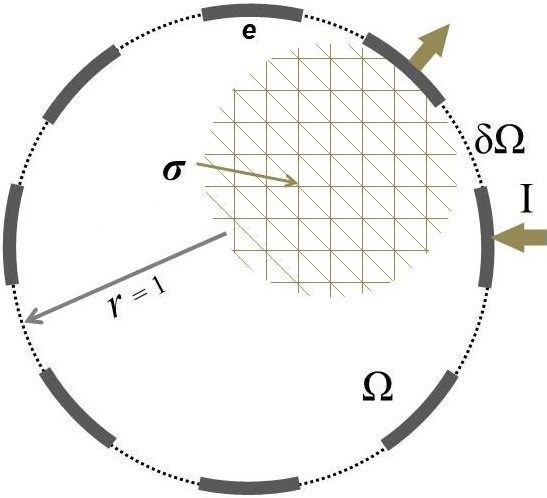
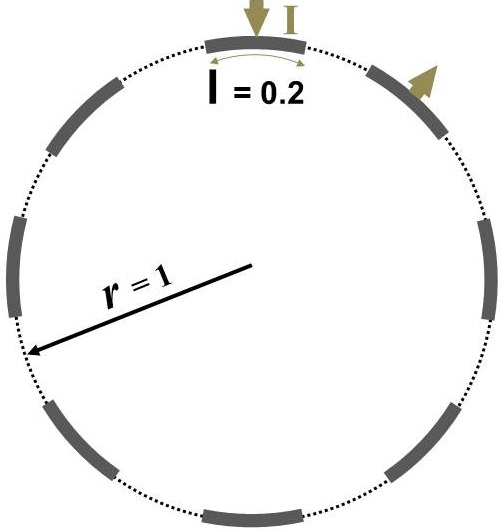
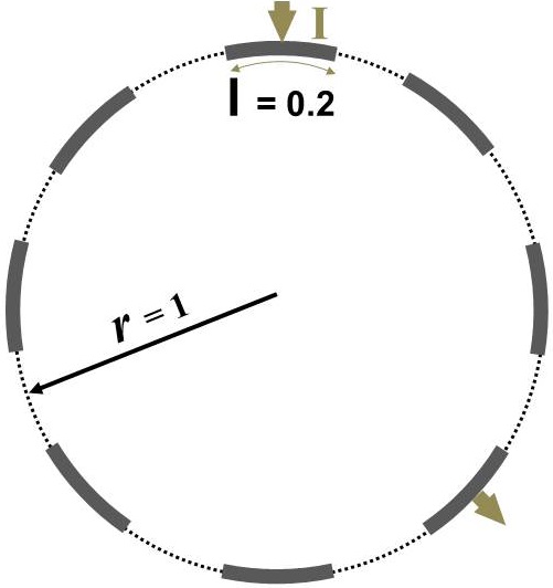
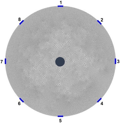
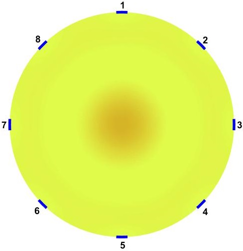
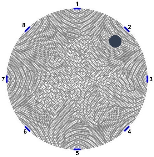
To simulate ERT experiments, a 2D domains is computationally simulated in this paper which is shown in Figure 1a. For simplicity, a symmetric circular ERT domain () with radius of 1 is considered. Eight equally spaced electrodes are positioned over the boundary (). The length of electrodes are kept constant as . The electrical conductivity distribution is constrained between (non-zero to avoid singularity). ERT measurements are applied on the domain with all current injection and potential measurement patterns possible. Current injection is considered as where current of amp injected from electrode and ejected form electrode ; , where is number of electrodes. Electrical potentials are measured at all electrodes for each current stimulations; , where stands for electrodes.
3 ERT complete electrode model
The Complete Electrode Model (CEM) is used which is the most accurate forward model for the ERT since it takes into account the effects of the electrodes and contact impedances [19, 18]. The CEM consists of the differential equation
| (1) |
and boundary conditions
| (2) |
| (3) |
| (4) |
where is the electrical conductivity, is the electric potential, is the outward unit normal, is the surface area under electrode, and , and , respectively, are the contact impedance, electric potential and total current corresponding to . Further, the charge conservation law must be satisfied, and the potential reference level needs to be fixed,
| (5) |
Here, Galerkin Finite Element Method (GFEM) with piecewise linear approximation of electrical conductivity and quadratic approximation for electrical potential is used to approximate the solution of the variational form of the forward model [20, 21, 22]. Using GFEM, the potential distribution within the object is approximated with the finite sum
| (6) |
and the potentials on the electrodes as
| (7) |
where the functions and are the basis functions and and are the nodal potential values of and . In Equation 6, is the number of nodes. Inserting these two approximative functions into the variational equations results in a system of linear equations which can be written in matrix form as
| (8) |
where are the electrical potentials. , where and is the vector of current of current stimulation pattern. K is the stiffness matrix which takes into account the effects of the electrodes and contact impedances between the object and the electrodes [19, 18]. Thus the approximation for the potentials are obtained by solving Equation 9
| (9) |
4 Distinguishability
Two conductivities and are distinguishable when the difference between their potential measurements exceeds the experimental percision of measurements, [17, 23, 24]. Equation 10 presents the distinguishability criterion, .
| (10) |
In [17, 23, 24], distinguishability is defined also as ”homogeneous of degree zero” to be the norm of the voltage measurement differences over electrodes divided by the norm of the power applied to . Therefore, distinguishability criterion remains neutral to the amplitude of current injection and projects the potential changes between two states of electrical conductivities. According to this definition, the most desirable ERT measurements have higher distinguishability.
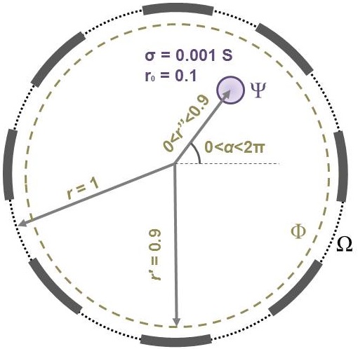
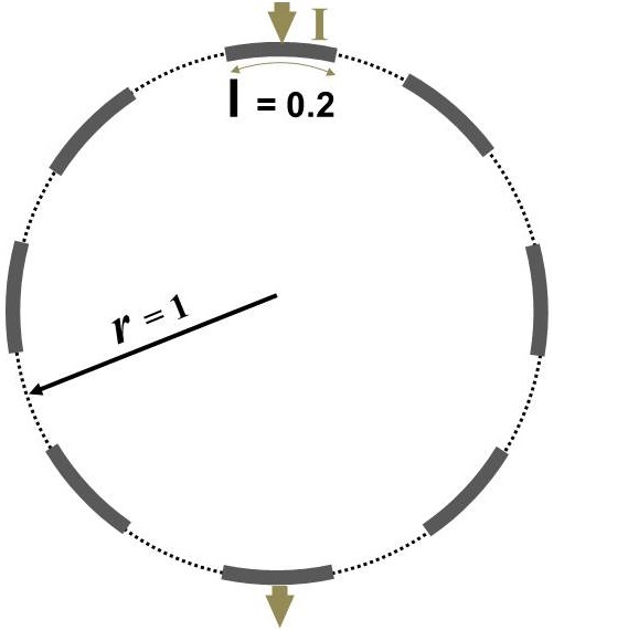
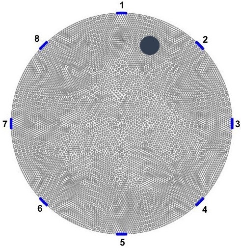
The distinguishability distribution over , can be estimated using Equation 10 between two conductivity distribution of and . refers to the original domain, and refers to the same domain that an anomaly with different conductivity is placed inside of it. Here, a circular anomaly inside the domain with radius of and electrical conductivity of 0.001 1 is moved inside over the entire domain (Figure 1b). The spatial distribution of distinguishability, , then is estimated over .
In this paper, we aim to maximize with respect to the optimal background electrical conductivity distribution of the domain. is maximized by maximizing . is maximized when the electrical power transferred through electrodes are maximized (Equation 11). Therefore, we maximize the energy transferred in the domain based on background conductivity distribution using a maximization algorithm of compliance matrix over the domain to optimize background conductivity distribution with constrained conductivity and subjected to the CEM forward model.
| (11) |
5 Optimization Problem
Equation 12 defines the compliance matrix, which is discretized FEM electrical power over the discretized domain, ,
| (12) |
In this section, the power-law approach is used to maximize as a function of in the domain.
Equation 5 shows the optimization of resulting in
which is subjected to:
| (13) | |||
where K is global stiffness matrix, and are the elements of potential vector and stiffness matrix, is the vector of design variable for electrical conductivity, and is tensor of electrical conductivities, is the number of elements and is penalization power which is normally 3 [15, 16]. is unit tensor of electrical conductivities, and and are designing target and initial assembled electrical conductivity respectively. is the constraint condition for volume fraction of electrical conductivity distributions. The optimization problem (Equation 5) is solved using standard Optimality Criteria method [15, 16].
A heuristic updating method for electrical conductivity is used based on Bendse [15] which is formulated as
| (14) |
where is incremental move limit, is a numerical damping coefficient and is found from the optimality condition as
| (15) |
The sensitivity of the objective function is found as
| (16) |
To ensure existence of unique solution and mesh independency for the optimization problem, a filtering method [16] is used to update element sensitivities as
| (17) |
where is the convolution operator which is
| (18) |
where and operator dist() is defined as the distance between centers of elements and . Therefore, the convolution operator is zero outside the filtering area () and decays linearly inside the filter area. The modified sensitivities are used in the Optimality Criteria update. depends on current stimulations, I. This means that for each , there is a . is the optimum background electrical conductivity of which may provide the highest for each .
For each ERT domain with current stimulations of , all of should be found. The final optimum electrical conductivity background, , is a nonlinear function of all . Finally, the is found by maximizing over all (Equation 5).
| which is subjected to: | |||
| (19) | |||
where , and are stacked global stiffness, potentials and current matrices for all current stimulations pattern of . The optimization problem similarly is solved using standard Optimality Criteria method. uses maximum amount of electrical power to transfer the injections for all current stimulation patterns which maximize the distribution over the sensor ().
6 ERT Inverse Problem
In order to study whether distinguishability enhancement can provide reconstructability enhancement, difference imaging reconstructions are provided in this paper. In difference imaging, we denote the conductivity distribution difference between before and after change by . In difference imaging, an approximate, linearized observation model for the difference potential measurement data is written as
| (20) |
where is the Jacobian matrix of the mapping between spatially discretized conductivity changes and , and is the measurement noise. Here, denotes the total number of potential measurements. Given the above model, the objective in difference imaging is to estimate based on the , which leads to a minimization problem
| (21) |
where is TV regularization functional related to the change of conductivity [25]. The Cholesky factor of the noise precision matrix is defined as , where , is the covariance of the noise.
Here, the regularization functional is selected as
| (22) |
which is a differentiable approximation of the isotropic TV functional [25]. Here, is the gradient of the at element in the FEM mesh. The choice of regularizing functional in Equation (21) depends on the application. In the present work, we use a TV regularization since the local anomaly change results in sharp boundary change. The regularization parameter is a weighting parameter which is chosen for all ERT reconstruction in this paper. is a small parameter that ensure TV is differentiable; is chosen as . In order to provide ERT reconstructions, the simulated experimental measurements are provided first with added normally distributed noise and with different forward model meshing from ERT difference imaging reconstructions.
7 Results and discussion
Section 5 described the approach to optimize electrical conductivity distribution. Results of the optimization problem clearly depend on several factors. Some of them were emphasized earlier in section 2 and illustrated by Figure 1. For purpose of topology optimization, the new factor, , should be defined as electrical conductivity fraction of optimized domain to initial domain. certainly plays an important role in topology optimization. The optimization problem above can be solved for different values which result in different topology optimization solutions. Therefore, for main part of this section we focus mainly on . means, topology optimization will result in an optimal design with of electrical conductivity distributions of uniform background conductivity of over the domain. But finally, we compare results for multiple designs for further discussion.
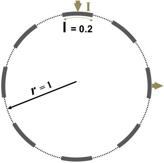
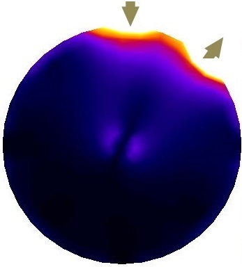
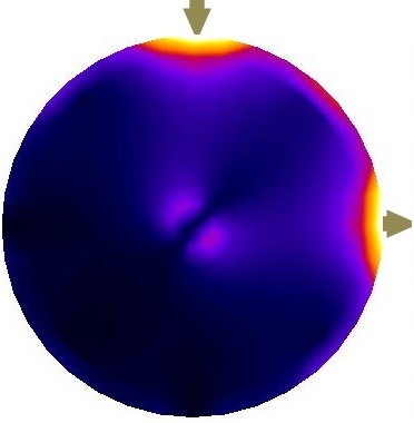
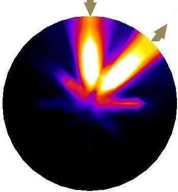
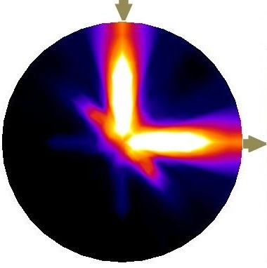
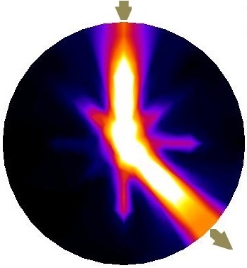
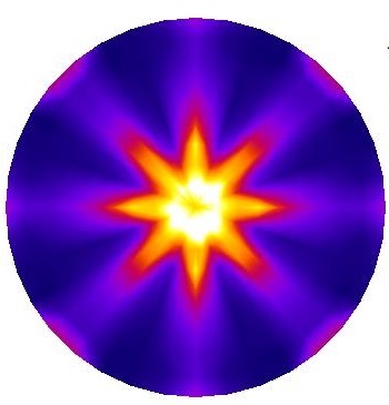
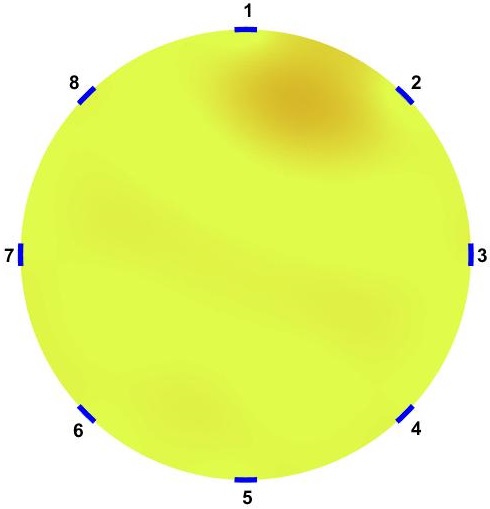
The domain shown in Figure 1 consists of a total of 56 patterns of current injections (). Current injection is one of the prominent variables in optimization of background conductivity because of its effect on electrical potentials at electrodes. First, we solve 56 individual optimization problems (Equation 5) to obtain for each current injections. Due to the symmetry, first 4 estimated corresponds to first set of current injections suffice to represent all corresponding to . The rest of 52 solutions are replications. Figure 2 shows the first four current stimulations and corresponding distributions with . Since stands for the background conductivity for maximum compliance inside the domain, it maximizes electrical potential of electrodes which in-turn maximizes .
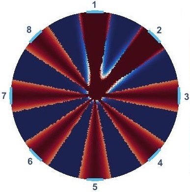
results presented by Figure 2 follow similar patterns and suggest periodic behavior in angular axis with higher conductivity closer to electrodes. Their differences come from different . Despite this difference, in all of them, the optimized background conductivity increases current density distribution at center of the domain. In circular domain, center has the lowest distinguishability [14]. The optimized provides a more uniform current density distribution specially at the center. This enables ERT to provide more useful information at electrodes which means eventually higher . The next step is to investigate whether the optimized provides a better distinguishability for the corresponds current stimulations than the uniform .
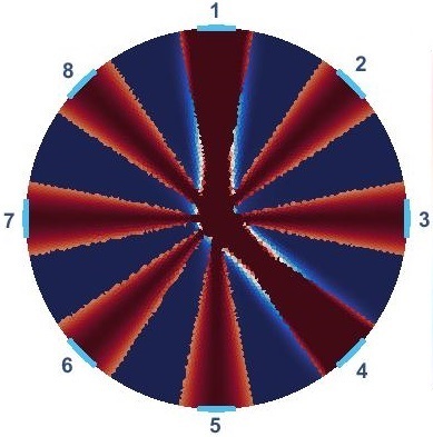
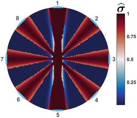
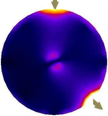
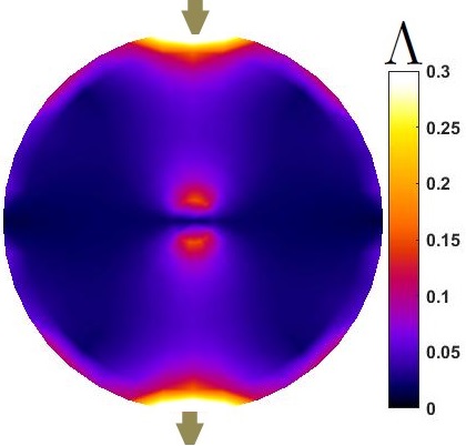
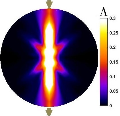
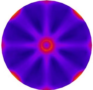
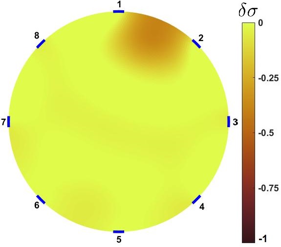
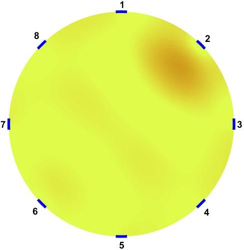
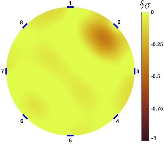
For this purpose, The anomaly () is moved inside for all and , and is measured (shown in Figure 1b). Figure 3 compares and distributions for all four current injection scenarios. In all four current injection scenarios, shows higher overall distinguishability (). provides maximum distinguishability at center and areas far from the boundaries for all the cases. This in fact is an advantage since ERT based sensors suffer from asymptotic loss of distinguishability with increase of size because distance of the interior of sensor increased from electrodes [24, 26]. Results suggest that maximizing compliance matrix of the sensors improve distinguishability of the areas far from electrodes.
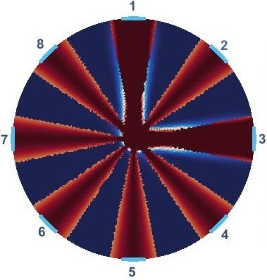
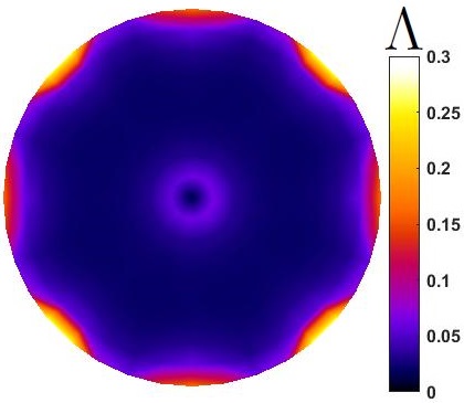
However, Figure 3 shows ; areas of with minimum 0.001 values of conductivity gain very low distinguishability which may become blinds spots. This may make more desirable than due to this issue. But, proposed results are from single current stimulations. Therefore, having multiple current stimulation patterns may fix this issue. Then, next step is to estimate corresponds to all current stimulations for case of which is shown by Figure 4.
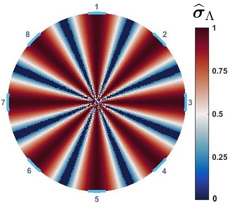
presents the optimum distribution of conductivity in the domain which maximizes electrical power function inside the sensor while improve performance and distinguishability of the sensor. is shown as a symmetric angular distribution of conductivity patterns. Electrical conductivity is higher angularly closer to the electrodes, which means these regions have more contribution in power transfer function. This pattern makes electrical current travel the most optimal path for each .
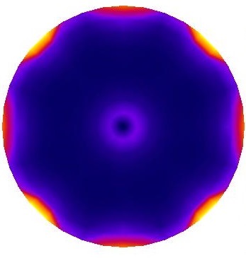
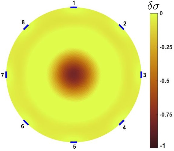
Figure 5 shows the corresponds distinguishability distributions of and . improves distinguishability from uniform background significantly. It specifically improves the values in lowest distinguishability areas which are over center region. Therefore, using full current stimulation patterns, using optimized sensors () provide more ”visibility”. This suggests that, with provided dimensions, number of electrodes and size of sensor, one way of improving the distinguishability of the sensor is engineered background electrical conductivity. This is an applicable approach to improve ERT sensor for application of large area sensing [6, 14]. This can show a possible application of these sensors for the cases that sensors will be used with higher probability of changes at certain regions of interest. Further, proposed results prove that, using with several current stimulation patterns provides even better distinguishability distribution.
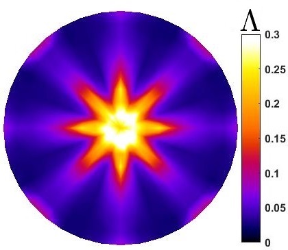
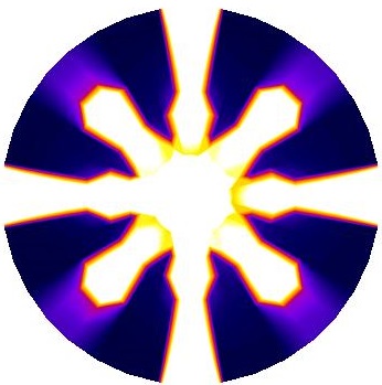
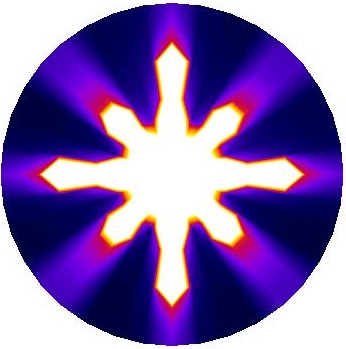
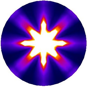
is a parameter in topology optimization which should be fixed as . means electrical conductivity distribution equal to whole fraction of uniform background distribution of . The constrained condition of provides the electrical conductivity fraction of the optimal background domain. Therefore, value of can affect the topology optimized answer and corresponding . Figure 6 compares distributions for equal to 1, 0.7, 0.6, 0.5, 0.4, and 0.2. means the uniform . Higher results in higher distinguishability over central regions. Although, in lower ranges of distinguishability increased at central parts but reduced significantly at the other regions. Comparing Figure 5 results, it can be shown that improves distinguishability all around the domain.
In order to study whether distinguishability enhancement can provide a better reconstructability, three difference imaging reconstructions are provided. The first column of Figure 7 presents two circular anomalies with 0.001 conductivity and radius in center and the edge of sensor. The anomalies were placed at center, close to edge between electrodes 1 and 2, and close to electrode 2 because these three spots have highest and lowest distinguishability values in optimized sensors (Figure 6). are reconstructed over uniform background conductivity of (second column of Figure 7). also reconstructed for optimized background conductivity with (third column of Figure 7), respectively. For all three cases, anomaly detected sharper and closer to real changes in than uniform background. These result can support the idea that distinguishability enhancement can provide reconstructability enhancement as well. Also, comparing both recosntruction cases suggests that using instead of uniform background does not reduce reconstruction ability of ERT over edges and it does not result in blind spots.
8 Conclusion
In this paper, we proposed an optimization approach for obtaining an optimal background conductivity distribution which results in highest distinguishability distribution for ERT based sensors. The proposed approach was evaluated using ERT simulations over a circular sensor with 8 electrodes. It has been shown that this approach provides the background conductivity distribution with higher distinguishability (). Also, the parameter as a designing target conductivity volume can affect the optimized results.
In proposed approach, the ERT domain topologically was optimized to maximize compliance matrix over the domain while kept the performance higher than uniform background domain. The higher performance is achieved because of better current density distribution over the domain which means that we measure more current density changes over the domain using optimized background conductivity. Also, we guide the current flow into the center of the domain which is furthest point from electrodes. In regular ERT domains, distinguishability decreased asymptotically as a function of distance to the electrodes. Therefore, proposed design improves distinguishability of the areas with least distinguishability expectations.
Results in Figure 5 suggests that with using less material and using optimum design we can improve distinguishability specially at most critical regions or regions of interest. The region of interest can be chosen as regions far from boundaries, ERT provides lowest distinguishability values, or any susceptible area of the domain. This approach, can be used for application which region of interest is available, which the customized design improves distinguishability over regions of interest. Using optimized ERT domain, distinguishability is improved at region of interest significantly and potentially we can achieve better reconstructability. It also enables ERT to be used for applications with higher amount of noises and using ERT experimentations with less of the experimental precision of measurements. Results in Figure 5 shows effect of values on final results.
Finally, ERT reconstructions were presented to investigate whether distinguishability enhancement can provide reconstructability enhancement. Difference imaging with TV regularization applied to both uniform and optimized background conductivity, and results suggest that optimized background conductivity may improve reconstructability.
References
References
- [1] D.S. Holder, Electrical Impedance Tomography: Methods, History and Applications, Medical Physics 32, 2731, 2005.
- [2] B.H. Brown, Electrical Impedance Tomography (EIT) – A Review, Journal of Medical Engineering & Technology 27 (3), 97-108, 2003.
- [3] M. Bodenstein, M. David, K. Markstaller Principles of electrical impedance tomography and its clinical application, Critical Care Medicine 37 (2), 713-724, 2009.
- [4] E.L. Costa, R.G. Lima, M.B. Amato Electrical impedance tomography, Current Opinion in Critical Care 15 (1), 18-24, 2009.
- [5] M. Hallaji and M. Pour-Ghaz, A new sensing skin for qualitative damage detection in concrete elements: Rapid difference imaging with electrical resistance tomography, NDT & E International 68, 13-21, 2014.
- [6] R. Rashetnia, O.K. Alla, G. Gonzalez-Berrios, A. Seppänen and M. Pour-Ghaz, Electrical Resistance Tomography–Based Sensing Skin with Internal Electrodes for Crack Detection in Large Structures, Materials Evaluation 76 (10), 1405-1413, 2018.
- [7] R. Rashetnia, O.K. Alla, G. Gonzalez-Berrios, A. Seppänen and M. Pour-Ghaz, Electrical Resistance Tomography Based Sensing Skin with Internal Electrodes for Crack Detection in Large Structures: Preliminary Results Standard Difference Imaging Study, 27th ASNT Research Symposium 170-181, 2018.
- [8] M. Cheney, D. Isaacson, J.C. Newell Electrical impedance tomography, Society for Industrial and Applied Mathematics 41 (1), 85-101, 1999.
- [9] V.A. Cherepenin, A.Y. Karpov, A.V. Korjenevsky, V.N. Kornienko, Y.S. Kultiasov, M.B. Ochapkin, O.V. Trochanova and J.D. Meister, Three-dimensional EIT imaging of breast tissues: system design and clinical testing, IEEE Transactions on Medical Imaging 21 (6), 662-667, 2002.
- [10] M. Hallaji, A. Seppänen and M. Pour-Ghaz, Electrical impedance tomography-based sensing skin for quantitative imaging of damage in concrete, Smart Materials and Structures 23 (8), 085001, 2014.
- [11] R. Rashetnia, M. Hallaji, D. Smyl, A. Seppänen and M. Pour-Ghaz, Detection and localization of changes in two-dimensional temperature distributions by electrical resistance tomography, Smart Materials and Structures 26 (11), 115021, 2017.
- [12] D. Liu, V. Kolehmainen, S. Siltanen and A. Seppänen, A nonlinear approach to difference imaging in EIT; assessment of the robustness in the presence of modelling errors, Inverse Problems 31 (3), 035012, 2015.
- [13] D. Liu, V. Kolehmainen, S. Siltanen, A.M. Laukkanen and A. Seppänen, Nonlinear difference imaging approach to three-dimensional electrical impedance tomography in the presence of geometric modeling errors, IEEE Transactions on Biomedical Engineering 63 (9), 1956-1965, 2015.
- [14] R. Rashetnia, Inverse Problems in Material System Monitoring with Applications in Damage Detection and Tomography, P.hD. Thesis North Carolina State University University, 2017.
- [15] M.P. Bendse, Optimization of structural topology, shape and material, Springer Berlin, Heidelberg, New York, 1995.
- [16] O. Sigmund, Design of material structures using topology optimization, P.hD. Thesis Department of Solid Mechanics, Technical University of Denmark, 1994.
- [17] D. Isaacson, Distinguishability of conductivities by electric current computed tomography, IEEE Transactions on Medical Imaging MI-5 (2), 91-95, 1986.
- [18] E. Somersalo, M. Cheney, and D. Isaacson, Existence and uniqueness for electrode models for electric current computed tomography, SIAM Journal on Applied Mathematics 52 (4), 1023-1040, 1992.
- [19] K.S. Cheng, D. Isaacson, J.C. Newell and D.G. Gisser, Electrode models for electric current computed tomography, IEEE Transactions on Biomedical Engineering 36 (9), 918-924, 1989.
- [20] P.J. Vauhkonen, M. Vauhkonen, T. Savolainen and J.P. Kaipio, Three-dimensional electrical impedance tomography based on the complete electrode model, IEEE Transactions on Biomedical Engineering 46, 1150-1160, 1999.
- [21] M. Vauhkonen, W. Lionheart, L. Heikkinen, P. Vauhkonen and J. Kaipio, A MATLAB package for the EIDORS project to reconstruct two-dimentional EIT images, Physiological Measurement 22, 107-111, 2001.
- [22] P.J. Vauhkonen, Image reconstruction in three-dimensional electrical impedance tomography, 951781304X University of Kuopio, 2004.
- [23] M. Cheney and D. Isaacson, Distinguishability in Impedance Imaging, IEEE Transactions on Biomedical Engineering 39 (8), 852-860, 1992.
- [24] H. Garde and K. Knudsen, Depth dependent bounds on distinguishability of inclusions in electrical impedance tomography, SIAM Journal of Applied Mathematics 77 (2), 697-720, 2017.
- [25] L.I. Rudin, S. Osher and E. Fatemi, Nonlinear total variation based noise removal algorithms, Physica D 60, 259-268, 1992.
- [26] H. Garde and S. Staboulis, Convergence and regularization for monotonicity-based shape reconstruction in electrical impedance tomography, Numerische Mathematik 135 (4), 1221–1251, 2017.