Topology Estimation of Simulated 4D Image Data by Combining Downscaling and Convolutional Neural Networks
Abstract
Four-dimensional image-type data can quickly become prohibitively large, and it may not be feasible to directly apply methods, such as persistent homology or convolutional neural networks, to determine the topological characteristics of these data because they can encounter complexity issues. This study aims to determine the Betti numbers of large four-dimensional image-type data. The experiments use synthetic data, and demonstrate that it is possible to circumvent these issues by applying downscaling methods to the data prior to training a convolutional neural network, even when persistent homology software indicates that downscaling can significantly alter the homology of the training data. When provided with downscaled test data, the neural network can estimate the Betti numbers of the original samples with reasonable accuracy.
Keywords: Betti numbers, topology, manifold, convolutional neural network, computer vision, persistent homology
1 Introduction
An understanding of the topological structure of image-type data can be critical in areas such as material science (Al-Sahlani et al., 2018; Duarte et al., 2020) and medicine (Cang and Wei, 2017; Lundervold and Lundervold, 2019), where methods such as Magnetic Resonance Imaging (MRI) and Computed Tomography (CT) may be used to determine the existence and shape of cavities within materials, or identify normal and pathological anatomical structures. By considering an -dimensional image as a manifold (or more accurately, as a manifold-with-boundary), its structural properties can be investigated from a topological perspective. MRI and CT scans offer examples of images in the 3D setting, as does real-time ultrasound (US), which captures 2D images over time to produce 3D image data; 3D images are comprised of voxels (the 3-dimensional (3D) analogue of a pixel).
In the 4D setting, 4D-US, functional-MRI, and 4D-CT offer methods to scan a 3D target over time to produce 4D image data; this affords the observation of processes and movements. These data are usually produced by collecting a synchronised sequence of 2D slices, which are then rectified into a 4D format by using slice timing correction techniques that employ various interpolation methods in order to accommodate for the time delay that is exhibited as each slice is captured (Pauli et al., 2016; Parker et al., 2017). 4D data can also occur if 2D or 3D data are equipped with other dimensions, and can also be the outcome of manifold learning (Lee and Verleysen, 2007).
In material science, micro-tomography has been used to observe the structural evolution of materials while they undergo hydration processes (Zhang et al., 2022), and to study the effect of exposure to load, temperature change, or current on manufactured porous materials, such as cellular materials and syntactic foams (Al-Sahlani et al., 2018; Duarte et al., 2020).
4D imaging also has applications in the medical diagnostic arena, where it may allow moving structures to be imaged over time. A review paper by Kwong et al. (2015) offers a broad look into how these dynamic imaging techniques can be used to observe visceral, musculo-skeletal, and vascular structures in order to assess joint instability and valve motion. An analysis of the topological characteristics of medical imaging is also a research consideration (Loughrey et al., 2021). For example, in cancer research, Kim et al. (2019) investigated the impact of topological data analysis in helping to differentiate between MRI scans of subjects with and without a genetic deletion event associated with a better glioma prognosis.
4D topological data analysis is a domain that may open a range of avenues for future research and improvements in applications that were previously restricted to 2D and 3D methods. Currently, the two main candidate techniques for topological data analysis in this area are persistent homology (Otter et al., 2017), and convolutional neural networks (CNNs). Unfortunately, 4D imaging can result in data that are dense, in that they capture vast regions of target material versus empty space, and data that require large amounts of storage. Furthermore, due to the additional dimension of the data in 4D, significant computational, memory, and time-complexity challenges of 4D topological data analysis methods need to be addressed.
The present study proposes and demonstrates the feasibility of an approach that combines the downscaling of large 4D image-type manifold data, which comprise of black-and-white toxels (the 4D analogue of a pixel), and the training of a 4D CNN, in order to estimate the topological characteristics of the data. In particular, all four dimensions of the data that we consider are treated equally; one could indeed inspect these data from any 4D perspective, and not necessarily assume that they arise from observing 3D samples as they evolve with time. In the context of this work, the term large data refers to data that is expensive, or even infeasible, to analyse in its raw form, because of computational or memory challenges (see Sections 2 and 3.3).
Although data analysis techniques have received significant attention in various area of science and mathematics, we are still in it early stages of exploring how to apply computer vision approaches to the task of estimating the topological characteristics of data, such as Betti numbers. The contributions that we provide in this work include:
-
•
the generation of large synthetic 4D data samples with non-trivial topologies,
-
•
training results that demonstrate that 4D CNNs can estimate the topology of the data even after downscaling,
-
•
a comparison with a representative persistent homology approach, and
-
•
a discussion that addresses some current limitations of the methods that we investigate, and provides motivation towards several potential future areas of research that may solve these issues.
While we specifically address the case of image-type data in this work, persistent homology-based methods may be more suitable for data in point-cloud or mesh format, as we discuss in the concluding paragraph of Section 2.
2 Background
Inspired by the structure of 3D data blocks in material science, the present study used simulated 4D data cubes, which could be described as the 4D analogue of a 3D foam or block of Swiss cheese. The boundaries of the cavities in such 4D data cubes are formed by 3-manifolds, which can be described and distinguished by using methods of algebraic and geometric topology (Hatcher, 2002). The topological classification of 3-manifolds was only achieved in 2003 (Bessieres et al., 2010) and the topology of objects in 4D can be much richer than in 2D or 3D. In the present study, we only consider some basic objects as part of our dataset generation, namely balls, that is, , and various tori that exist in 4D, including , , and . However, these manifolds are already topologically more complex than what would usually be considered in machine learning, for example, as the outcome of manifold learning (Lee and Verleysen, 2007).
The Betti numbers are a concept in algebraic topology that capture the essential structure of a manifold or topological space given by the holes of the manifold or topological space (Edelsbrunner and Harer, 2010). The th Betti number is often denoted by , where is the number of path-connected components that comprise a topological space, and are the number of -dimensional holes in the space. Holes are formalised in algebraic topology, where roughly speaking, a -dimensional cycle is a closed submanifold, a -dimensional boundary is a cycle that is also the boundary of a submanifold, and a -dimensional homology class is an equivalence class of the group of cycles modulo the group of boundaries , otherwise known as the th homology group . Any non-trivial homology class represents a cycle that is not a boundary, or equivalently, a -dimensional hole. can be defined as the rank of the group (Edelsbrunner and Harer, 2010). In this work, the term hole will be used in its homological sense, and the term cavity will refer to the result of ‘cutting-out’ of the interior of a sample. For example, the introduction of a donut-shaped cavity into a 3D sample, that is , will result in the introduction of a 1D hole and a 2D hole. In , only the first four Betti numbers are relevant, and their relationship to the Euler characteristic is given by
Persistent homology is a computational approach with which one can derive topological indices, such as the Betti numbers, of the underlying manifold of data. The theoretical complexity of applying persistent homology using a sparse implementation is cubic in the number simplices that describe a sample, however, in practice, this can be as low as linear (Zomorodian and Carlsson, 2005). A general introduction that can serve as background to computational topology and algebraic topology can be found in the books of Edelsbrunner and Harer (2010) and Hatcher (2002), respectively.
The use of CNNs to predict the Betti numbers of data was first proposed by Paul and Chalup (2019), who trained 2D and 3D CNNs with simulated data cubes into which cavities were introduced. This approach was extended by Hannouch and Chalup (2023), who used simulated 4D data cubes to train a custom 4D CNN that was implemented using the Pytorch library (Paszke et al., 2019). Both studies used persistent homology software (JavaPlex (Adams et al., 2014) and GUDHI (Maria et al., 2014), respectively) as a comparison partner, and discuss some of the headwinds that were faced when using both persistent homology software and CNNs. When analysing image-type data with persistent homology, it was possible to gain some memory and speed advantage by using a single (unfiltered) cubical complex (Otter et al., 2017; Hannouch and Chalup, 2023). Notwithstanding, these headwinds appear to magnify in the 4D setting, where the computational and memory demands of analysing samples larger than became prohibitively large, even when aided by supercomputers.
Persistent homology algorithms are often used to summarise some of the topological and geometrical attributes of a dataset by distilling them into a visual output, and there is evidence that subsampling methods can be effective when used to compute averaged persistence images (Chazal et al., 2015), diagrams (Cao and Monod, 2022) and landscapes (Solomon et al., 2022) of point-cloud data. Moitra et al. (2018) proposed a clustering approach to facilitate the persistent homology algorithm, and Nandakumar (2022) explored sampling techniques in the multi-parameter context. In the present study, we consider standard downsampling and average-pooling techniques to downscale large 4D image-type manifold data, and demonstrate that while persistent homology algorithms may begin to break down when analysing the global topology of these downscaled data (that is, they may compute results that are vastly different from those attributed to the original data), CNNs appear to better tolerate the use of these techniques as a means to mitigate the limitations that are faced when estimating the Betti numbers of these data. While more sophisticated downscaling approaches do exist in the 2D image setting, such as content-adaptive (Kopf et al., 2013), perceptually-based (Öztireli and Gross, 2015), and detail-preserving (Weber et al., 2016) algorithms, the techniques considered in this work offer an early look into how pre-processing 4D image-type data may afford the analysis of larger samples, with potentially higher resolutions, or a greater number of cavities. As we will discuss later in Section 5, our results also serve to motivate an investigation into the use of these other algorithms, along with other machine learning approaches, as they may complement the results that are presented here.
Manifold Formula Volume Simplification to where and
3 Dataset generation
Data generation software was implemented in Python using data structures from the NumPy library (Harris et al., 2020) to represent 4D data cubes as images, and apply vector and matrix operations. Beginning with a ‘solid’ 4D cube (represented by a 4D tensor with every entry set to 1), a random number of cavities were introduced into the cube by setting the entries that represented the cavities to 0. Each cavity was homeomorphic to one of the objects in Table 1, and was randomly scaled and rotated before being positioned. The resulting cube was a 4D generalisation of a single-channelled, black-and-white image.
3.1 Design
Data design experiments were focused on choosing radius parameters (namely, , , and ) that would generate samples with non-trivial topologies in a resolution that would ensure that holes were represented clearly (in a homological sense). Since the toxels of an image were attributed integral coordinates, persistent homology software would, theoretically, be capable of correctly detecting holes of any dimension, provided that the diameter of a hole was greater than the distance between diagonal points of a 4D unit-cube ( units). Otherwise, calculations would suffer as a result of there being insufficient resolution to describe a hole with such a small radius. Conversely, if parameters were too large, then the cavities would be so big that we would be limited to samples with fewer holes and less interesting topologies.
Table 1 provides several formulas that may be used to depict a variety of 4D objects in an -system, and were used to design the cavities for the dataset. These objects vary in their geometry (relative to each other), and this can be demonstrated by experimenting with the parameters in each formula. For example, does not have a tunnel, whereas does have a tunnel and can vary from being quite ‘flat and expansive’ to being more ‘round’, depending on the choice of the parameter , which sets the orientation of the factor and ranges from to . Figure 1 shows several 2D visualisations that offer some intuition of how varying can impact the resulting embedding of (and, equivalently, ) in . The idea is to begin with a (dark-grey) torus that is oriented according to , and positioned units from the origin along the -axis in the 3D -hyperplane. The torus is then rotated around the origin, through the -plane, in order to introduce the third factor. Although the figures may suggest otherwise, the implicit formula for that is used to generate our data guarantees that overlaps or self-intersections do not occur. This is because we are working in , rather than , as the figures may also suggest; the extra dimension cannot be shown easily in 2D. Figure 1a demonstrates a construction in which , and Figures 1b and 1c demonstrate constructions in which ; notice that Figure 1c is, in fact, a radians -rotation of Figure 1b. Because of the symmetry of the torus that we begin with, any -rotation of the construction in Figure 1a is inconsequential, as is a radians -rotation of the remaining examples. In practice, we only need to consider when ranges from to ; the remaining options arise freely from the random rotations that are applied during data generation.
3.2 Hypervolumes
In order to maintain some homogeneity in the range of sizes of these objects, we selected parameters for each object that would produce cavities with a similar range of hypervolume (4D-volume). Formulas for the hypervolumes of these objects, along with some simplifications that arise by setting (for and ) are also provided in Table 1. For , we assume that , and that the value of depends on and ranges from to . Therefore, for , the hypervolume of ranged from to .
The hypervolumes of the remaining objects were scaled into the same range by finding suitable values for . For example, if the hypervolume of were to also fall within this range, it was necessary to choose such that . Rearranging this expression leads to Equation 1, and the remaining ranges were deduced in the same way.
| (1) |
| (2) |
| (3) |
3.3 Dataset parameters
The parameters that we selected in order to generate a 4D dataset with which to investigate our approach are summarised in Table 2. Our study focused on recognising the global topology of compact manifolds. Hence, we restricted our experiments to single-component samples (), and ensured that both a cube’s boundaries were not disturbed and that cavities did not intersect each other. These rules were enforced by implementing a 1-toxel boundary and minimum 6.5-unit spacing between cavities. The self-intersection of a cavity was prevented via the simplifications that were explained in Section 3.2. The choices for and , as listed in the row of the column of Table 2, were sufficient to produce cavities with a nice resolution.
Cube Parameters 32000 samples : 7.6 to 24.1 : 8.4 to 26.7 : 6.4 to 20.3 : 4.8 to 25.6 1 toxel boundary : 4.2 to 13.3 : 3.2 to 10.1 : 4.8 to 12.8 1 to 48 holes : 2.4 to 6.4 6.5 unit spacing : 0 to
Each sample comprised of a 4D cube, with the combined number of 1D, 2D, and 3D holes ranging from 1 to 48. A cube was used because it was large enough to contain a non-trivial range of cavities, which afforded the analysis of samples with interesting topologies. This data was also slightly bigger than what would have been feasible to be directly analysed using persistent homology methods or CNNs with our hardware (NVIDIA DGX Station, with an Intel Xeon E5-2698 v4 CPU, 256GB RAM, and four V100-32GB GPUs). Hence, downscaling became a requirement in order to process this data. Note also that the cavity dimensions were small enough that the application of downscaling could potentially disturb the homology of a sample by closing up holes (see Section 4.1).
The data was generated in parallel on a High Performance Computing (HPC) Grid in 100-sample batches, over 320 nodes. An average of 8.60 hours was required to complete each batch, and the entire process utilised approximately 2753.21 HPC hours.
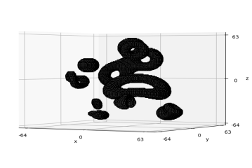
A visualisation of the cavities within a sample is shown in Figure 2. This is achieved by inverting the toxel values (setting 0 to 1, and vice versa) so that the cube itself is stripped away in order to reveal the objects that were used to produce its cavities, and then taking 3D slices along some axis. In this case, 18 equally-spaced slices have been taken along the -axis. Taking finer slices allows one to see a more continuous-looking evolution of the cavities (see Appendix A).


3.4 Data labelling
Each label was produced on-the-fly during the generation of a sample. The homology of each cavity that was introduced into a sample was algebraically derived by, firstly, observing that the 4D cube is homeomorphic to the 4D ball, and therefore shares the same homology. Secondly, the homology of both the object being considered for removal and its boundary were computed by using the Künneth theorem. Thirdly, the Mayer-Vietoris Sequence was applied to find the homology of the cube with the cavity ; an introduction to the theorems that were used in this derivation can be found in Hatcher (2002). The results of these calculations are provided in Table 3. Since the Betti numbers that each cavity contributed to a sample were known, they could simply be summed over their dimensions in order to produce a label for the sample. Furthermore, the parameters outlined in Table 2 were large enough to always produce a homologically correct representation in the cube setting. Consequentially, there was no requirement to analyse the samples using persistent homology software in order to produce a label. A more detailed description of the mathematics involved in producing the labels, can be obtained from Hannouch and Chalup (2023).
| Manifold | |||||
|---|---|---|---|---|---|
| 3-Sphere | 1 | 0 | 0 | 1 | 0 |
| 4-Ball | 1 | 0 | 0 | 0 | 1 |
| 1 | 0 | 0 | 1 | 0 | |
| 1 | 1 | 1 | 1 | 0 | |
| 1 | 1 | 0 | 0 | 0 | |
| 1 | 0 | 1 | 0 | 2 | |
| 1 | 0 | 1 | 1 | 1 | |
| 1 | 1 | 0 | 1 | -1 | |
| 1 | 3 | 3 | 1 | 0 | |
| 1 | 2 | 1 | 0 | 0 | |
| 1 | 1 | 2 | 1 | 1 |
4 Experiments and results
The goal of this work was to explore whether downscaling techniques could be useful in circumventing the complexity issues that make the application of persistent homology and machine learning software difficult when analysing the topological characteristics of large 4D image-type manifold data. Two downscaling approaches were considered: downsampling, and average-pooling. The GUDHI persistent homology Python library was used to determine how consistent the sample labels were with their downsampled image; a cubical complex was used because of its suitability to image-type data (Otter et al., 2017). The persistent homology algorithm operated over a single cubical complex, which comprised only of cubical simplexes between contiguous voxels with a value equal to 1, that is, the cubical complex was completely determined by the voxels themselves. Therefore, in theory, any persistent homology software would have applied the algorithm to the same complex and yielded the same result.
4.1 Downsampling approach
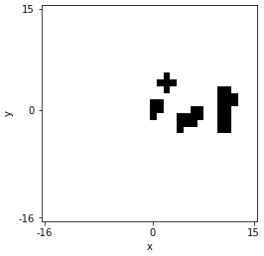
The data were downsampled from to by taking the voxels at every 4th coordinate along each axis; the resulting images were 256 times smaller. Figure 3 gives an indication of how course-looking a 3D slice of a 4D sample becomes after the application of this degree of downsampling. Labels were not modified, however, the impact of downsampling was investigated using GUDHI. This was performed in parallel on a HPC Grid in 50-sample batches, over 640 nodes. An average of 0.66 hours was required to analyse each batch, and the entire process utilised approximately 420.14 HPC hours. As summarised in Table 4, all of the samples remained as single-component images (), however, the number of samples with a structure that was consistent their label for , , and was markedly affected, with only 16065 (50.2%), 14154 (44.23%), and 4121 (12.88%) samples matching their label for each respective Betti number. Only 2175 (6.8%) of the samples still possessed a structure that was completely consistent with their label; this result is recorded in the ‘complete match’ column.


| Combined accuracy | Complete match | ||||
|---|---|---|---|---|---|
| 100.0 | 50.2 | 44.23 | 12.88 | 51.83 | 6.8 |
The downsampled data was then used to train a 4D CNN, which was implemented with PyTorch, and had a similar architecture to the 2D and 3D CNNs that were used by Paul and Chalup (2019); these consisted of several convolution layers, followed by a max-pooling layer, and finishing with a sequence of fully connected linear layers. Our models began with four iterations of a module consisting of: a 4D convolution layer, followed by a ReLU activation function, and then a 4D max-pooling layer. The convolutional layers output 8, 16, 32, and 64 channels, respectively, with 2 units of padding and a kernel. The pooling kernel was units. After the fourth convolution module, the result was flattened, and then passed through two fully connected layers that were separated by a ReLU operation. Finally, the result was output to a sparsely coded vector by reserving one output neuron for each possible value of . Based on the design of our dataset, we accommodated for the values 0 and 1 for , and accommodated for the values 0 to 16 for , , and .
Full-scale deep learning experiments were performed on the above-mentioned NVIDIA DGX Station using a multi-GPU arrangement. A high-bandwidth connection between the GPUs, and between the GPUs and CPU, via NVLink, made it possible to consider these devices as a single, larger, computing element, which was able to accommodate the CNN and allow for a 192-sample batch size.
The dataset was randomly divided into 90% training, 5% validation, and 5% test sets at the beginning of each experiment. For each epoch, the samples were rotated in random multiples of 90 degrees through a randomly selected coordinate plane as they were fed into the Pytorch dataloader; this offered twelve possible variations on each sample. The Cross Entropy loss function was appropriately set up to handle the four separate outputs for , and . The Adam optimiser was initialised with a learning rate of 0.001, and a scheduler was employed to reduce the learning rate by a factor of 10 at epochs 160 and 190 over a 200 epoch training schedule.
Table 5 presents the test set accuracy average and standard deviation that were achieved in five repeats of the experiment. Each experiment required just over 4 days (approximately 98 hours) to complete, and utilised its own randomly selected training set, validation set, and test set in the proportions set out above. An average combined test set accuracy of 82.41% was achieved.
| Run | Combined accuracy | ||||
|---|---|---|---|---|---|
| 1 | 100.0 | 76.97 | 61.92 | 78.18 | 79.27 |
| 2 | 100.0 | 83.85 | 74.19 | 83.04 | 85.27 |
| 3 | 100.0 | 72.45 | 60.94 | 77.6 | 77.75 |
| 4 | 100.0 | 87.62 | 68.52 | 87.09 | 85.81 |
| 5 | 100.0 | 85.13 | 65.34 | 85.3 | 83.94 |
| 100.0 | 81.2 | 66.18 | 82.25 | 82.41 | |
| 0.0 | 5.62 | 4.82 | 3.78 | 3.28 |
4.2 Average-pooling approach
Similar experiments were performed with another downscaled dataset that was produced by reducing the same samples to via 4D average-pooling; the software that was used to perform this version of downscaling was implemented with Pytorch. The labels were, again, left unaltered. The resulting samples were a smaller, blurry, grey-scale image of the original cube. Figure 4 depicts a sequence of 2D slices, each taken from the cubes that were produced by downsampling and average-pooling the same 4D sample that was the subject of Figure 3. For comparison, Figure 4 shows equally-spaced 2D slices (taken from bottom to top) of the same downsampled 3D slice that is seen in the left of Figure 3, and compares these slices with their corresponding average-pooled slice. The average-pooled slices appear to be less coarse and richer in features, versus their corresponding downsampled slice. For example, the first downsampled slice is empty, however, the average-pooled slice contains evidence of a cavity; the fifth, sixth, and eighth slices demonstrate something similar. The seventh and tenth downsampled slices contain pairs of features that are actually part of the same cavity, which we deduce by inspecting the corresponding average-pooled slice. This occurs because, while downsampling only collects the value (0 or 1) of the voxels at every fourth coordinate, the average-pooling kernel (with a 4-unit stride) takes an average of the voxel values that it sees.
| Downsampled | Average-pooled |


|


|


|


|


|


|


|


|

|


|
The dataset division percentages, CNN architecture, and scheduler that were detailed in Section 4.1 were also used for these experiments, however in this case, the Adam optimiser was initialised with a learning rate of 0.0001 in response to inconsistent results that were observed during several abbreviated preliminary test runs with a learning rate of 0.001. Despite the smaller learning rate, the scheduler performed the same 200 epochs. The final results of these experiments are presented in Table 6, along with some statistics. An average combined accuracy of approximately 78.52% was observed in these experiments.
| Run | Combined accuracy | ||||
|---|---|---|---|---|---|
| 1 | 100.0 | 61.69 | 61.57 | 82.87 | 76.53 |
| 2 | 100.0 | 58.85 | 59.9 | 79.34 | 74.52 |
| 3 | 100.0 | 67.59 | 67.53 | 85.3 | 80.11 |
| 4 | 100.0 | 70.72 | 72.8 | 88.48 | 83.0 |
| 5 | 100.0 | 66.2 | 63.89 | 83.68 | 78.44 |
| 100.0 | 65.01 | 65.14 | 83.94 | 78.52 | |
| 0.0 | 4.23 | 4.61 | 3.0 | 2.92 |
4.3 Efficacy of CNNs
In order to understand how well the CNN was able to perform, several 1000-sample datasets of cubes were again generated from cubes via the downsampling approach described in Section 4.1; these data were therefore new to the trained models. As expected, an analysis of these datasets, using both GUDHI and a trained CNN, produced similar results to those presented in Tables 4 and 5. Despite the significant inconsistency between the structure of these downsampled images and their labels (only 7.5% of the new samples exhibited a complete label match after downsampling, as demonstrated by GUDHI), the CNN was still able to achieve a complete match for over 65% of the samples, and more accurately estimated the respective Betti numbers of each sample versus the results produced via persistent homology (see Table 7).
| Combined accuracy | Complete match | |||||
|---|---|---|---|---|---|---|
| GUDHI | 100.0 | 50.5 | 43.94 | 14.84 | 52.32 | 7.52 |
| CNN | 100.0 | 91.74 | 78.26 | 92.78 | 90.7 | 68.34 |
Benchmarking the two proposed downscaling options was not the aim of this work, however, the CNN architecture, and many of the training hyperparameters, were left unchanged across the training experiments. We observed that average-pooling produced a slightly better estimation, which, possibly, could have been a consequence of the richer-looking data (as demonstrated in Figure 4), although, this CNN also performed worse when estimating . We also note that the randomness that was applied during dataset generation and subsetting, or changing the CNN architecture, could have produced different results. Overall, the test set accuracy that was achieved in the downsampling experiment was comparably similar to the results that were achieved in the average-pooling experiment (82.41% versus 78.52%), therefore, both options could be equally as useful.
5 Discussion
Provided the availability of appropriate computing resources, and if prior knowledge or a preliminary analysis of data identifies that features of interest, such as the holes, are large enough or captured in a high enough resolution to tolerate downscaling, then persistent homology may still be a suitable option; for example, this may be true when analysing materials that are manufactured under known conditions or to specification.
If synthetic data, which sufficiently models 4D real-world data, is acquired, then a computer vision approach may be a suitable approach to estimating the Betti numbers of the data; this may follow similar efforts to those in the 3D data generation context (Gao et al., 2022; Bissaker et al., 2022). The results of our work demonstrate that it may also be possible to apply downscaling methods prior to employing CNNs to estimate the Betti numbers of 4D image-type manifold data on which it may not be possible to directly apply existing methods, or where downscaling is too disruptive; our samples were reduced by a factor of 256. The representative comparison with persistent homology software demonstrates that the machine learning approach, using CNNs that are trained on simulated data, appears to be more robust to the homological changes resulting from downscaling, with the CNN achieving an average combined accuracy of over 80%, and a complete-match accuracy of nearly 70%, despite the significant discrepancies between the structure of downscaled training data and their original labels. Downsampling also granted the use of persistent homology software, however, only about 50% and 7% accuracy were achieved for the same metrics.
The application of downscaling may prove to be useful in cases where it may be less critical to determine the exact topology of data, such as in material science, or where it is already appropriate to consider the results of persistent homology less explicitly, for example, via persistence images, as demonstrated in the analysis of data derived from dynamical systems (Adams et al., 2017).
5.1 Limitations
The results and insights that have been presented in this work extend the approach that was pioneered by Paul and Chalup (2019) in the 2D and 3D setting. Collectively, these results have, primarily, been restricted to synthetic, single-component samples. More complicated features, such as multiple-components, links, and connected sums, or the use of topology-preserving deformations to vary the geometric appearance of cavities, are yet to be considered in this line of research. Addressing this would be essential in order to apply the CNN approach more generally to the task of estimating homology; it is likely that real data may possess these features. For example, the random deformation of the canonical embeddings that are used in our experiments could be accomplished by developing a 4D version of the repulsive tangent-point energy algorithm that was proposed by Yu et al. (2021b, a) (although, we concede that this method itself would be computationally expensive, and would not protect against the homological consequences of producing deformed cavities with self-intersections).
Although we have demonstrated that it is possible to analyse large 4D samples with CNNs where using existing options may not be feasible, it is apparent from our work that the process of generating synthetic data with which to train a CNN comes at a significant resource and time cost that may not be accessible to everyone. Choosing how to generate data that models real data may also be a necessary preliminary step, which brings with it a new set of challenges. In our case, we faced the complication of finding a balance between the size of the data that we considered, and the size of the CNN that we used. The decision to use a relatively simple CNN architecture in our experiments was made in order to demonstrate how readily CNNs could be applied to our task, but was also a result of being confined to the VRAM capacity of the available hardware; introducing additional layers, connections, or training parameters would potentially increase the hardware requirements. In the near term, performance gains could be achieved through improved software engineering. In the long term, improvements may come in the form of cost reduction and hardware advances, which would certainly make exploring deeper, wider, or more sophisticated 4D CNN architectures, similar to the many well-established options that are available in lower-dimensions (Simonyan and Zisserman, 2014; Szegedy et al., 2015; He et al., 2016), more tractable; the hope would be to determine which architectures cope best with topological applications, such as estimating Betti numbers.
5.2 Future work
As previously alluded to, there are several immediate directions into which the results that are presented in this work could be extended in future work. The downscaling results could be expanded by implementing, and then exploring the use of, the 4D equivalents of other image downscaling algorithms, such as those that were mentioned in Section 2. The downscaling approach that we took in this work could also be compared and combined with multi-view methods, which employ lower-dimensional representations of data that are produced by gathering lower-dimensional images from different angles (perspectives), or by projecting 4D data onto a lower-dimensional space; this could potentially offer some speed or memory advantage. This would contrast volumetric approaches that process 4D data using 4D operations, such as those applied through a 4D CNN (see Section I.B of Cao et al. (2020) for a discussion about multi-view and volumetric approaches). In the 3D setting, Su et al. (2015) demonstrate how CAD and voxel data may be projected onto two dimensions by using an ‘outside’ perspective to capture several images of the data from different angles in a similar way to taking X-ray scans of a subject along three orthogonal axes. Alternatively, Shi et al. (2015) project 3D samples outwards from their centre onto an annulus that wraps around the object. Similar ideas have been employed by Qi et al. (2016) and Kanezaki et al. (2018). Nevertheless, Wang et al. (2019) suggest that standard volumetric approaches may be more capable of gathering information when compared to multi-view models, and argue that this is because multi-view strategies often fail to encode information from different views. It may, however, be easier to implement larger models in lower dimensions, or exploit pre-trained models by fine-tuning (Russakovsky et al., 2015; Brock et al., 2016), which could potentially be useful when handling large 4D data.
More generally, several other matters also require deeper investigation in order to fully assess the capabilities of CNNs in estimating topology. For one, the task of modelling a real dataset for the purpose of training a CNN would need to be addressed. Secondly, generating this data would need to be carefully controlled, possibly via some form of topology-preserving algorithm; this itself raises the question of whether generating a diverse training dataset from the outset, that is, a dataset that comprises of more complicated features, such as multiple components, links, and connected sums, could be enough to train a CNN that is capable of general homology estimation, without the need to understand any properties of the real dataset under consideration. These aspects could, potentially, benefit from a (Bayesian) statistical approach, such as those considered in zero-shot, one-shot, or -shot learning models (Fe-Fei et al., 2003; Palatucci et al., 2009), which are capable of generalising knowledge to unfamiliar cases after seeing little, or no, training examples without requiring extensive retraining, or where complete training may not be possible due to dataset limitations, or because real data may be infinitely-variable (as may be the case with homeomorphic deformations).
6 Conclusion
When samples become large, as is typical for 4D data, the hardware requirements to train CNNs with this data can also grow. Similarly, it can become difficult to meet the computational and memory demands of traditional topological data analysis techniques, such as persistent homology. Alleviating these issues in the context of large point-cloud data is an active area of research (Cao and Monod, 2022; Solomon et al., 2022; Moitra et al., 2018; Chazal et al., 2015); the results of our study apply to image-type data and run in parallel to this line of research.
Although we could demonstrate that downscaling and 4D CNNs work well together when determining the topology of manifolds in our 4D simulated data, the approach would still have computational constraints when it would come to large real-world samples in 4D. Future research could expand on more advanced data generation techniques, which are capable of producing more diverse-looking datasets. When coupled with more sophisticated CNN architectures and more powerful hardware, it may be possible to produce even more capable computer vision-based solutions in 4D.
Acknowledgments and Disclosure of Funding
This project was supported by the Australian Research Council Discovery Project Grant DP210103304 ‘Estimating the Topology of Low-Dimensional Data Using Deep Neural Networks’. The first author was supported by a PhD scholarship from the University of Newcastle associated with this grant.
Appendix A Visualising 4D samples
By inverting the toxel values of a sample (setting 0 to 1, and vice versa), we are able to visualise the cavities within a sample. The supplementary material of this paper includes a link to a short video, which depicts the 4D sample that was presented in Figure 2 by visualising each of the 128 slices along the -axis as a 3D frame. This allows us to see examples of the balls and various tori that have been used to cut-out cavities from the interior of a 4D cube.
References
- Adams et al. (2014) H. Adams, A. Tausz, and M. Vejdemo-Johansson. JavaPlex: A research software package for persistent (co)homology. In H. Hong and C. Yap, editors, Mathematical Software – ICMS 2014, pages 129–136, Berlin, Heidelberg, 2014. Springer Berlin Heidelberg. ISBN 978-3-662-44199-2.
- Adams et al. (2017) H. Adams, T. Emerson, M. Kirby, R. Neville, C. Peterson, P. Shipman, S. Chepushtanova, E. Hanson, F. Motta, and L. Ziegelmeier. Persistence images: A stable vector representation of persistent homology. Journal of Machine Learning Research, 18(8):1–35, 2017. URL http://jmlr.org/papers/v18/16-337.html.
- Al-Sahlani et al. (2018) K. Al-Sahlani, S. Broxtermann, D. Lell, and T. Fiedler. Effects of particle size on the microstructure and mechanical properties of expanded glass-metal syntactic foams. Materials Science and Engineering: A, 728:80 – 87, 2018. ISSN 0921-5093. URL https://doi.org/10.1016/j.msea.2018.04.103.
- Bessieres et al. (2010) L. Bessieres, G. Besson, M. Boileau, S. Maillot, and J. Porti. Geometrisation of 3-Manifolds, volume 13 of EMS Tracts in Mathematics. European Mathematical Society, Zurich, 2010. URL https://www-fourier.ujf-grenoble.fr/~besson/book.pdf.
- Bissaker et al. (2022) E. J. Bissaker, B. P. Lamichhane, and D. R. Jenkins. Connectivity aware simulated annealing kernel methods for coke microstructure generation. In A. Clark, Z. Jovanoski, and J. Bunder, editors, Proceedings of the 15th Biennial Engineering Mathematics and Applications Conference, EMAC-2021, volume 63 of ANZIAM J., pages C123–C137, jul 2022. doi: 10.21914/anziamj.v63.17187. URL http://journal.austms.org.au/ojs/index.php/ANZIAMJ/article/view/17187.
- Brock et al. (2016) A. Brock, T. Lim, J. M. Ritchie, and N. Weston. Generative and discriminative voxel modelling with convolutional neural networks. arXiv preprint arXiv:1608.04236, 2016.
- Cang and Wei (2017) Z. Cang and G.-W. Wei. TopologyNet: Topology based deep convolutional and multi-task neural networks for biomolecular property predictions. PLOS Computational Biology, 13(7):1–27, 07 2017. URL https://doi.org/10.1371/journal.pcbi.1005690.
- Cao et al. (2020) W. Cao, Z. Yan, Z. He, and Z. He. A comprehensive survey on geometric deep learning. IEEE Access, 8:35929–35949, 2020.
- Cao and Monod (2022) Y. Cao and A. Monod. Approximating persistent homology for large datasets. arXiv preprint arXiv:2204.09155, 2022.
- Chazal et al. (2015) F. Chazal, B. Fasy, F. Lecci, B. Michel, A. Rinaldo, and L. Wasserman. Subsampling methods for persistent homology. In F. Bach and D. Blei, editors, Proceedings of the 32nd International Conference on Machine Learning, volume 37 of Proceedings of Machine Learning Research, pages 2143–2151, Lille, France, 07–09 Jul 2015. PMLR. URL https://proceedings.mlr.press/v37/chazal15.html.
- Duarte et al. (2020) I. Duarte, T. Fiedler, L. Krstulović-Opara, and M. Vesenjak. Cellular metals: Fabrication, properties and applications. Metals, 10(11):1545, 2020.
- Edelsbrunner and Harer (2010) H. Edelsbrunner and J. Harer. Computational Topology: An Introduction. Applied Mathematics. American Mathematical Society, 2010. ISBN 9780821849255.
- Fe-Fei et al. (2003) L. Fe-Fei et al. A Bayesian approach to unsupervised one-shot learning of object categories. In Proceedings Ninth IEEE International Conference on Computer Vision, pages 1134–1141. IEEE, 2003.
- Gao et al. (2022) D. Gao, J. Chen, Z. Dong, and H. Lin. Connectivity-guaranteed porous synthesis in free form model by persistent homology. Computers & Graphics, 106:33–44, 2022. ISSN 0097-8493. URL https://www.sciencedirect.com/science/article/pii/S0097849322000917.
- Hannouch and Chalup (2023) K. M. Hannouch and S. Chalup. Learning to see topological properties in 4D using convolutional neural networks. In 2nd Annual Topology, Algebra, and Geometry in Machine Learning Workshop at ICML 2023, Proceedings of Machine Learning Research. PMLR, 2023. Accepted 19.06.2023.
- Harris et al. (2020) C. R. Harris, K. J. Millman, S. J. van der Walt, R. Gommers, P. Virtanen, D. Cournapeau, E. Wieser, J. Taylor, S. Berg, N. J. Smith, R. Kern, M. Picus, S. Hoyer, M. H. van Kerkwijk, M. Brett, A. Haldane, J. F. del Río, M. Wiebe, P. Peterson, P. Gérard-Marchant, K. Sheppard, T. Reddy, W. Weckesser, H. Abbasi, C. Gohlke, and T. E. Oliphant. Array programming with NumPy. Nature, 585(7825):357–362, Sept. 2020. URL https://doi.org/10.1038/s41586-020-2649-2.
- Hatcher (2002) A. Hatcher. Algebraic Topology. Cambridge University Press, Cambridge, UK, 2002.
- He et al. (2016) K. He, X. Zhang, S. Ren, and J. Sun. Deep residual learning for image recognition. In Proceedings of the IEEE Conference on Computer Vision and Pattern Recognition, pages 770–778, 2016.
- Kanezaki et al. (2018) A. Kanezaki, Y. Matsushita, and Y. Nishida. Rotationnet: Joint object categorization and pose estimation using multiviews from unsupervised viewpoints. In Proceedings of the IEEE Conference on Computer Vision and Pattern Recognition, pages 5010–5019, 2018.
- Kim et al. (2019) D. Kim, N. Wang, V. Ravikumar, D. Raghuram, J. Li, A. Patel, R. E. Wendt III, G. Rao, and A. Rao. Prediction of 1p/19q codeletion in diffuse glioma patients using pre-operative multiparametric magnetic resonance imaging. Frontiers in Computational Neuroscience, 13:52, 2019.
- Kopf et al. (2013) J. Kopf, A. Shamir, and P. Peers. Content-adaptive image downscaling. ACM Transactions on Graphics, 32(6):1–8, 2013.
- Kwong et al. (2015) Y. Kwong, A. O. Mel, G. Wheeler, and J. M. Troupis. Four-dimensional computed tomography (4DCT): A review of the current status and applications. Journal of Medical Imaging and Radiation Oncology, 59(5):545–554, 2015. URL https://onlinelibrary.wiley.com/doi/abs/10.1111/1754-9485.12326.
- Lee and Verleysen (2007) J. A. Lee and M. Verleysen. Nonlinear Dimensionality Reduction. Information Science and Statistics. Springer, 2007. ISBN 978-0-387-39350-6.
- Loughrey et al. (2021) C. F. Loughrey, P. Fitzpatrick, N. Orr, and A. Jurek-Loughrey. The topology of data: opportunities for cancer research. Bioinformatics, 37(19):3091–3098, 2021.
- Lundervold and Lundervold (2019) A. S. Lundervold and A. Lundervold. An overview of deep learning in medical imaging focusing on MRI. Zeitschrift für Medizinische Physik, 29(2):102–127, 2019.
- Maria et al. (2014) C. Maria, J. Boissonnat, M. Glisse, and M. Yvinec. The GUDHI library: Simplicial complexes and persistent homology. In Mathematical Software - ICMS 2014 - 4th International Congress, Seoul, South Korea, August 5-9, 2014. Proceedings, volume 8592 of Lecture Notes in Computer Science, pages 167–174. Springer, 2014. URL https://doi.org/10.1007/978-3-662-44199-2_28.
- Moitra et al. (2018) A. Moitra, N. O. Malott, and P. A. Wilsey. Cluster-based data reduction for persistent homology. In 2018 IEEE International Conference on Big Data (Big Data), pages 327–334, 2018. doi: 10.1109/BigData.2018.8622440.
- Nandakumar (2022) V. Nandakumar. On subsampling and inference for multiparameter persistence homology. In ICLR 2022 Workshop on Geometrical and Topological Representation Learning, 2022. URL https://openreview.net/forum?id=BxNa4-JTgc.
- Otter et al. (2017) N. Otter, M. A. Porter, U. Tillmann, P. Grindrod, and H. A. Harrington. A roadmap for the computation of persistent homology. EPJ Data Science, 6:17–55, 2017. URL https://doi.org/10.1140/epjds/s13688-017-0109-5.
- Öztireli and Gross (2015) A. C. Öztireli and M. Gross. Perceptually based downscaling of images. ACM Transactions on Graphics, 34(4), Jul 2015. ISSN 0730-0301. URL https://doi.org/10.1145/2766891.
- Palatucci et al. (2009) M. Palatucci, D. Pomerleau, G. E. Hinton, and T. M. Mitchell. Zero-shot learning with semantic output codes. In Y. Bengio, D. Schuurmans, J. Lafferty, C. Williams, and A. Culotta, editors, Advances in Neural Information Processing Systems, volume 22, pages 1410––1418. Curran Associates, Inc., 2009. URL https://proceedings.neurips.cc/paper_files/paper/2009/file/1543843a4723ed2ab08e18053ae6dc5b-Paper.pdf.
- Parker et al. (2017) D. Parker, X. Liu, and Q. R. Razlighi. Optimal slice timing correction and its interaction with fMRI parameters and artifacts. Medical Image Analysis, 35:434–445, 2017.
- Paszke et al. (2019) A. Paszke, S. Gross, F. Massa, A. Lerer, J. Bradbury, G. Chanan, T. Killeen, Z. Lin, N. Gimelshein, L. Antiga, A. Desmaison, A. Kopf, E. Yang, Z. DeVito, M. Raison, A. Tejani, S. Chilamkurthy, B. Steiner, L. Fang, J. Bai, and S. Chintala. PyTorch: An imperative style, high-performance deep learning library. In H. Wallach, H. Larochelle, A. Beygelzimer, F. d'Alché-Buc, E. Fox, and R. Garnett, editors, Advances in Neural Information Processing Systems 32, pages 8024–8035. Curran Associates, Inc., 2019. URL http://papers.neurips.cc/paper/9015-pytorch-an-imperative-style-high-performance-deep-learning-library.pdf.
- Paul and Chalup (2019) R. Paul and S. Chalup. Estimating Betti numbers using deep learning. In 2019 International Joint Conference on Neural Networks (IJCNN), pages 1–7. IEEE, 2019.
- Pauli et al. (2016) R. Pauli, A. Bowring, R. Reynolds, G. Chen, T. E. Nichols, and C. Maumet. Exploring fMRI results space: 31 variants of an fMRI analysis in AFNI, FSL, and SPM. Frontiers in Neuroinformatics, 10:24, 2016.
- Qi et al. (2016) C. R. Qi, H. Su, M. Nießner, A. Dai, M. Yan, and L. J. Guibas. Volumetric and multi-view CNNs for object classification on 3D data. In Proceedings of the IEEE Conference on Computer Vision and Pattern Recognition, pages 5648–5656, 2016.
- Russakovsky et al. (2015) O. Russakovsky, J. Deng, H. Su, J. Krause, S. Satheesh, S. Ma, Z. Huang, A. Karpathy, A. Khosla, M. Bernstein, et al. Imagenet large scale visual recognition challenge. International Journal of Computer Vision, 115(3):211–252, 2015.
- Shi et al. (2015) B. Shi, S. Bai, Z. Zhou, and X. Bai. Deeppano: Deep panoramic representation for 3D shape recognition. IEEE Signal Processing Letters, 22(12):2339–2343, 2015.
- Simonyan and Zisserman (2014) K. Simonyan and A. Zisserman. Very deep convolutional networks for large-scale image recognition. arXiv preprint arXiv:1409.1556, 2014.
- Solomon et al. (2022) E. Solomon, A. Wagner, and P. Bendich. From Geometry to Topology: Inverse Theorems for Distributed Persistence. In X. Goaoc and M. Kerber, editors, 38th International Symposium on Computational Geometry (SoCG 2022), volume 224 of Leibniz International Proceedings in Informatics (LIPIcs), pages 61:1–61:16, Dagstuhl, Germany, 2022. Schloss Dagstuhl – Leibniz-Zentrum für Informatik. ISBN 978-3-95977-227-3. doi: 10.4230/LIPIcs.SoCG.2022.61. URL https://drops.dagstuhl.de/opus/volltexte/2022/16069.
- Su et al. (2015) H. Su, S. Maji, E. Kalogerakis, and E. Learned-Miller. Multi-view convolutional neural networks for 3D shape recognition. In Proceedings of the IEEE International Conference on Computer Vision, pages 945–953, 2015.
- Szegedy et al. (2015) C. Szegedy, W. Liu, Y. Jia, P. Sermanet, S. Reed, D. Anguelov, D. Erhan, V. Vanhoucke, and A. Rabinovich. Going deeper with convolutions. In Proceedings of the IEEE Conference on Computer Vision and Pattern Recognition, pages 1–9, 2015.
- Wang et al. (2019) C. Wang, M. Pelillo, and K. Siddiqi. Dominant set clustering and pooling for multi-view 3D object recognition. arXiv preprint arXiv:1906.01592, 2019.
- Weber et al. (2016) N. Weber, M. Waechter, S. C. Amend, S. Guthe, and M. Goesele. Rapid, detail-preserving image downscaling. ACM Transactions on Graphics, 35(6), dec 2016. ISSN 0730-0301. URL https://doi.org/10.1145/2980179.2980239.
- Yu et al. (2021a) C. Yu, C. Brakensiek, H. Schumacher, and K. Crane. Repulsive surfaces. ACM Transactions on Graphics (TOG), 40(6):1–19, 2021a.
- Yu et al. (2021b) C. Yu, H. Schumacher, and K. Crane. Repulsive curves. ACM Transactions on Graphics (TOG), 40(2):1–21, 2021b.
- Zhang et al. (2022) L. Zhang, L. Wang, B. Yang, S. Niu, Y. Han, and S.-K. Oh. Rapid construction of 4D high-quality microstructural image for cement hydration using partial information registration. Pattern Recognition, 124:108471, 2022. ISSN 0031-3203. doi: https://doi.org/10.1016/j.patcog.2021.108471. URL https://www.sciencedirect.com/science/article/pii/S0031320321006476.
- Zomorodian and Carlsson (2005) A. Zomorodian and G. Carlsson. Computing persistent homology. Discrete & Computational Geometry, 33(2):249–274, 2005.