Topology and Spectrum in Measurement-Induced Phase Transitions
Abstract
Competition among repetitive measurements of noncommuting observables and unitary dynamics can give rise to a rich variety of entanglement phases. We here characterize topological phases in monitored quantum systems by their spectrum and many-body topological invariants. We analyze (1+1)-dimensional monitored circuits for Majorana fermions, which have topological and trivial area-law entangled phases and a critical phase with sub-volume-law entanglement, through the Lyapunov spectrum. We uncover the presence (absence) of edge-localized zero modes inside the bulk gap in the topological (trivial) area-law phase and a bulk gapless spectrum in the critical phase. Furthermore, by suitably exploiting the fermion parity with twisted measurement outcomes at the boundary, we construct a topological invariant that sharply distinguishes the two area-law phases and dynamically characterizes the critical phase. Our work thus paves the way to extend the bulk-edge correspondence for topological phases from equilibrium to monitored quantum dynamics.
Introduction.–
Topology is undoubtedly one of the most essential concepts in understanding stable phases of matter [1]. For ground states of local Hamiltonians with a finite excitation gap, states belonging to distinct topological phases cannot be smoothly deformed to each other without closing the gap, owing to discrete characters of their topological invariants [2]. In particular, for symmetry-protected topological phases [3, 4, 5, 6, 7, 8], nontrivial topology of the bulk leads to gapless boundary states robust against any symmetry-preserving perturbations. This phenomenon, known as the bulk-edge correspondence, has remarkable consequences in physical properties of the topological phases and has been intensively studied in the past few decades [9, 10, 11, 12, 13].
Despite notable successes in equilibrium systems, topology in out-of-equilibrium systems caused by external environment has yet to be fully understood. In particular, it is still elusive how the topology plays a role in monitored quantum systems, which gather a recent extensive interest as they host novel non-equilibrium phases concerning, e.g., entanglement [14, 15, 16, 17, 18, 19, 20, 21, 22, 23, 24, 25]. Indeed, repetitive measurements stabilizing distinct topological phases can lead to phase transitions between different entanglement phases, which can be probed by topological entanglement entropy or purification dynamics [26, 27, 28, 29, 30, 31, 32, 33, 34, 35, 36, 37, 38, 39, 40, 41, 42] (see also [43, 44, 45]). However, intrinsic spatiotemporal randomness caused by the probabilistic nature of measurement outcomes makes it difficult to generalize more standard notions of topological phases, such as bulk topological invariants and gapless edge modes, to monitored systems.
In this Letter, we discover gapless edge modes and a bulk topological invariant that characterize measurement-induced phase transitions of monitored Majorana circuits and discuss their bulk-edge correspondence. Introducing effective Hamiltonians obtained through the Lyapunov analysis, we reveal the presence (absence) of edge-localized zero modes inside the bulk gap in the topological (trivial) area-law phase. We also construct a bulk topological invariant based on the fermion parity, extending the method in equilibrium systems to the monitored setting; this is accomplished by introducing a unique boundary condition with twisted measurement outcomes. The invariant sharply distinguishes these gapped area-law phases, featuring the bulk-edge correspondence. Moreover, we show that the critical entanglement phase corresponds to a gapless phase concerning the Lyapunov spectrum. While the bulk-edge correspondence is obscured in this phase, we demonstrate that the topological invariant can still dynamically characterize the two gapped and gapless phases. Our result is summarized in Fig. 1.
Model and Lyapunov analysis.–
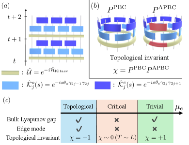
We consider a -dimensional quantum circuit acting on Majorana fermions [see Fig. 1(a)], consisting of repeated applications of three elementary steps: (i) unitary time evolution , (ii) measurements of all Majorana pairs on odd bonds, and (iii) measurements of all Majorana pairs on even bonds. These operations update to in a single time step. To be more precise, the unitary evolution is given by the Kitaev chain Hamiltonian, , with
| (1) |
where are Majorana fermions obeying and are real constants. The measurements of Majorana pairs on odd/even bonds with an outcome are described by the Kraus operators,
| (2) |
which are weak measurements of the strength . We set hereafter. Given a (unnormalized) state , each outcome is obtained with the Born probability, In the following, we use three boundary conditions: open (OBC), periodic (PBC), and antiperiodic (APBC). For the unitary evolution , the boundary condition is simply specified by : and for the OBC, PBC, and APBC, respectively. For the measurements, the OBC means that we discard from the circuit, while we need a careful definition of the APBC, as explained later.
At the time , an initial state is evolved by the Kraus operator labeled by a sequence of outcomes with ,
| (3) |
Since both unitary evolution and measurements are bilinear in Majorana fermions, this circuit maps a fermionic Gaussian state to another Gaussian state [46, 47, 48, 49, 50, 51, 52]. A fermionic Gaussian state is completely characterized by the Majorana covariance matrix whose element reads . Time evolution of the (unnormalized) Gaussian state is encoded in the transformation of the Majorana fermions, , where
| (4) |
Here, and are real antisymmetric matrices defined through and with (see Supplemental Material [53]).
Since this circuit is a product of random matrices, we can perform the Lyapunov analysis [54, 55, 56, 57, 58, 59, 60]. Provided that the Oseledec theorem [61, 62, 63] holds, the Lyapunov spectrum does not depend on the sequence of outcomes . It is also related to the energy spectrum of the effective Hamiltonian,
| (5) |
and the corresponding many-body Hamiltonian . Since is real antisymmetric, its eigenvalues come in pairs, . This defines the single-particle energy spectrum , which in the asymptotic limit coincides with the Lyapunov spectrum: . We below arrange them as . We can also compute the corresponding Lyapunov vectors . Written in the matrix form , they give in the asymptotic limit an orthogonal matrix that brings into the standard form,
| (6) |
In practice, we construct through computing Lyapunov vectors corresponding to the non-negative Lyapunov spectrum based on the complex fermion representation, which is equivalent to the Majorana representation [53]. In the following, the initial state of the trajectories is fixed to be a vacuum state , whereas the Lyapunov analysis itself is performed with random initial vectors for a given trajectory. We only look at a single trajectory specified by a typical sequence of and consider a temporal average of quantities in the long-time limit unless otherwise mentioned [53].
Lyapunov edge modes in measurement-only circuits.–
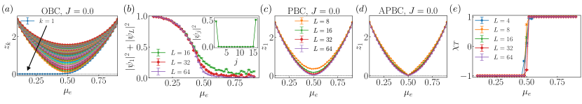
We first perform the Lyapunov analysis for the measurement-only circuit (). In this case, a direct transition at occurs from a topological to a trivial area-law phase, as numerically checked by the topological entanglement entropy and bipartite mutual information [53], as done in [41, 34, 42].
Remarkably, we reveal that the topological area-law phase is characterized by Majorana zero modes for the Lyapunov spectrum. Figure 2(a) shows the non-negative single-particle Lyapunov spectrum against for the measurement-only circuit under the OBC for . Importantly, takes a finite value for , while it vanishes for . Vanishing of under the OBC in the topological area-law phase implies the many-body Lyapunov gap closing for , which is reminiscent of Majorana zero modes for the static Kitaev chain [64].
We next show that the above zero mode is a spatially localized edge mode by analyzing the spinor wavefunction [65] with its element corresponding to the lowest energy . In Fig. 2(b), We plot the long-time average of the sum of the squared amplitudes for at both edges, , against . Deep inside the topological phase (), it takes a value close to regardless of the system size, signaling localization of the zero mode near the edges. In contrast, it decreases toward a value in the trivial phase, indicating that the Majorana mode delocalizes over the whole lattice on average. The localization of the zero modes in the topological phase is much more visible if we directly look at the spatial profile of the . The inset of Fig. 2(b) shows (trajectory-averaged) values of for and . These results indicate that the Lyapunov spectrum clearly reveals edge-localized Majorana zero modes in the topological area-law phase.
Topological invariant and bluk-edge correspondence.–
We now introduce a bulk topological invariant and relate it with the presence (absence) of the Lyapunov edge modes in the topological (trivial) area-law phase. Since the circuit conserves the fermion parity , the eigenstates of the effective Hamiltonian have definite parities unless they are degenerate. We then define the topological invariant as a difference between the fermion parities computed for the ground state under the PBC and that under the APBC. While this is analogous to the procedure for static Kitaev chains [64, 66, 67], a special care is required to determine the APBC because the trajectories depend on measurement outcomes. Namely, the APBC is here defined with respect to the PBC; we generate a circuit under the PBC with a sequence of measurement outcomes . Then the circuit under the APBC is defined by flipping the outcomes only for the boundary Majorana pairs, , with under the APBC. Using defined through the above prescription, we introduce the topological invariant as the product of their ground states’ parities. Since the parity can be computed as the sign of the Pfaffian of the single-particle Hamiltonian for noninteracting systems, which is known as Kitaev’s formula [64], the topological invariant for monitored Majorana circuits is given by
| (7) |
However, the explicit form of is numerically intractable for large . Thus, we instead compute defined by
| (8) | ||||
| (9) |
Since approximates and converges to for , we will also call as the topological invariant. We note that is not an orthogonal matrix for general .
In Fig. 2(c,d), we show the lowest single-particle Lyapunov spectrum for the measurement-only circuit under the (c) PBC and (d) APBC. It takes a finite value for both cases, implying a finite bulk Lyapunov gap, within each area-law phase. As shown in Fig. 2(e), the topological invariant clearly separates the topological and trivial area-law phases. Note that these results are qualitatively independent of the measurement outcomes . In fact, is satisfied in the whole parameter region, since the gap does not close at the transition for PBC due to finite-size splitting . On the other hand, abruptly changes from to across the transition point for APBC, implying an exact gap closing near . This results in the observed transition in . The behaviors of the bulk Lyapunov gap resemble those of the bulk energy gap of the static translation-invariant Kitaev chain [64]; in that case, for PBC and for APBC at the transition, across which the Pfaffian invariant changes its sign.
The edge-localized zero mode under the OBC in Fig. 2(a,b) and the topological invariant in Fig. 2(e) indicate that the bulk-edge correspondence applies even to nonequilibrium phases under temporally random measurements, if the bulk gap is open. Such an exploration based on topology in random dynamics is accomplished by the Lyapunov analysis and the appropriate definition of the topological invariant via effective Hamiltonians. Note that a naive quantity with does not provide a good topological invariant in general. Rather, focusing on the trajectory under the APBC dependent on the trajectory under PBC makes their fermion parities meaningful to define the invariant under random measurements.
Gapless critical phase with additional unitary.–
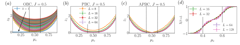
We now study the monitored circuit with unitary dynamics by the Kitaev Hamiltonian and discuss how the Lyapunov spectrum and the topological invariant behave. Reference [51] considered a continuous-time version of our model to find three different entanglement phases as increases. Specifically, the unitary part leads to a critical phase whose entanglement scales as between the topological and trivial area-law phases (see also [37, 38, 68, 69, 39, 70, 40, 41, 71, 42]). In our circuit model, we numerically find three entanglement phases separated by two transition points and for , using the topological entanglement entropy and bipartite mutual information [53].
To discuss the topology of the three phases, we first investigate the Lyapunov spectrum in the circuit with OBC, finding that the critical phase corresponds to a gapless phase without Majorana zero modes. Figure 3(a) shows the depedence of the non-negative single-particle Lyapunov spectrum. As observed in the measurement-only case, the lowest mode become gapless (gapped) in the topological (trivial) phase. In the critical phase for , not only the lowest mode but also higher modes appear to become gapless, implying the closing of the bulk Lyapunov gap. Interestingly, the -dependence of seems different between the topological area-law phase and the critical phase; decays faster than power law in the topological area-law phase (), while it appears to decay in for our available system sizes in the critical phase () [53].
The above observation of the bulk spectrum is also confirmed from the lowest spectrum under the PBC and APBC. Indeed, as shown in Fig. 3(b,c), goes to zero for , whereas the bulk gap is open for other . While the scaling form of right at the transitions and is close to , it appears to decay faster than inside the critical phase (except the APBC circuit at , where exact gap closing is anticipated nearby) [53].
The above results for the spectral gaps indicate that the bulk-edge correspondence is obscured for the gapless phase if we consider for finite , which is confirmed to be convergent irrespective of . That is, since can only be exactly zero near for APBC, the asymptotic topological invariant can switch the sign only at this point for finite system sizes. Indeed, we have numerically observed that flows towards for and for as increases [53]. In contrast, as discussed above, the Majorana zero mode seems absent even for . Therefore, while the critical phase is unstable in static Majorana chains and is thus unique to monitored Majorana chains, the bulk-edge correspondence is obscured since it corresponds to the gapless phase. This is reminiscent of the fact that topological phase is usually well defined in the gapped phase in static systems.
Remarkably, however, we find that the topological invariant dynamically characterizes the different phases, including the critical gapless phase. Specifically, we consider the sample-averaged invariant, , for the timescale . Figure 3(d) shows for different system sizes, from which we find three crossings with and . The locations of the first and last crossings coincide well to the transitions between the area-law gapped phases and critical gapless phase. Notably, this characterization is attributed to the divergent relaxation time of the invariant in the gapless phase. If we denote the timescale as , it is at least longer than , which increases faster than inside the gapless phase. Therefore, will not converge and almost stay zero for the gapless phase. This is contrasted to the gapped phases with , where rapidly converge to for . Note that the crossing point at is different from the boundaries of the three phases. The above argument indicates that this crossing is a finite-size artifact, and will flatly become zero in the entire critical phase for .
Summary and outlook.–
We have shown that monitored Majorana circuits in the gapped phases exhibit the bulk-edge correspondence through investigating the Lyapunov spectrum, gapless edge modes, and topological invariants based on the fermion parity. To define the topological invariant, we have used a unique methodology where the trajectory under APBC is defined with respect to that under PBC, according to twisted measurement outcomes at the boundary. We have also shown that the critical phase corresponds to the gapless phase in terms of the Lyapunov spectrum and is dynamically characterized by the topological invariant in a timescale .
Our study opens the way to explore topological features in monitored systems through the Lyapunov analysis. An important future direction is to examine many-body systems, where our topological invariant based on the twisted measurement outcomes readily applies. For example, it is intriguing to analyze monitored circuits with symmetry, for which measurements can stabilize an area-law phase with a symmetry-protected topological order of the cluster state [26, 38, 32]. Such a topological area-law phase will be charactarized by (nearly) four-fold degenerate Lyapunov spectrum under the OBC from gapless edge modes and a topological invariant measuring the change of one charge by twisting boundary measurement outcomes for another symmetry.
Note added.— While this work was in its final stage, we learned about a recent paper which investigates a similar issue [72].
Data availability.— Data and simulation codes are available upon reasonable request.
Acknowledgements.
Acknowledgments— We thank Xhek Turkeshi, Henning Schomerus, Alessandro Romito, Amos Chan, Keiji Saito, Ken Shiozaki, and Takahiro Morimoto for valuable discussions and comments. We thank Zhenyu Xiao and Kohei Kawabata for coordinating the submission of this work and Ref. [72]. H.O. is supported by RIKEN Junior Research Associate Program. K. M. and R.H. are supported by JST ERATO Grant Number JPMJER2302, Japan. K.M. is supported by JSPS KAKENHI Grant No. JP23K13037. R.H. is supported by JSPS KAKENHI Grant No. JP24K16982. Y.F. is supported by JSPS KAKENHI Grants No. JP20K14402 and No. JP24K06897. Part of the computation has been performed using the facilities of the Supercomputer Center, the Institute for Solid State Physics, the University of Tokyo.References
- Wen [2017] X.-G. Wen, Colloquium: Zoo of quantum-topological phases of matter, Rev. Mod. Phys. 89, 041004 (2017).
- Chen et al. [2010] X. Chen, Z.-C. Gu, and X.-G. Wen, Local unitary transformation, long-range quantum entanglement, wave function renormalization, and topological order, Phys. Rev. B 82, 155138 (2010).
- Gu and Wen [2009] Z.-C. Gu and X.-G. Wen, Tensor-entanglement-filtering renormalization approach and symmetry-protected topological order, Phys. Rev. B 80, 155131 (2009).
- Pollmann et al. [2010] F. Pollmann, A. M. Turner, E. Berg, and M. Oshikawa, Entanglement spectrum of a topological phase in one dimension, Phys. Rev. B 81, 064439 (2010).
- Chen et al. [2011] X. Chen, Z.-C. Gu, and X.-G. Wen, Classification of gapped symmetric phases in one-dimensional spin systems, Phys. Rev. B 83, 035107 (2011).
- Fidkowski and Kitaev [2011] L. Fidkowski and A. Kitaev, Topological phases of fermions in one dimension, Phys. Rev. B 83, 075103 (2011).
- Lu and Vishwanath [2012] Y.-M. Lu and A. Vishwanath, Theory and classification of interacting integer topological phases in two dimensions: A Chern-Simons approach, Phys. Rev. B 86, 125119 (2012).
- Chen et al. [2013] X. Chen, Z.-C. Gu, Z.-X. Liu, and X.-G. Wen, Symmetry protected topological orders and the group cohomology of their symmetry group, Phys. Rev. B 87, 155114 (2013).
- Hasan and Kane [2010] M. Z. Hasan and C. L. Kane, Colloquium: Topological insulators, Rev. Mod. Phys. 82, 3045 (2010).
- Qi and Zhang [2011] X.-L. Qi and S.-C. Zhang, Topological insulators and superconductors, Rev. Mod. Phys. 83, 1057 (2011).
- Senthil [2015] T. Senthil, Symmetry-Protected Topological Phases of Quantum Matter, Ann. Rev. Condens. Matter Phys. 6, 299 (2015).
- Witten [2016] E. Witten, Fermion path integrals and topological phases, Rev. Mod. Phys. 88, 035001 (2016).
- Chiu et al. [2016] C.-K. Chiu, J. C. Y. Teo, A. P. Schnyder, and S. Ryu, Classification of topological quantum matter with symmetries, Rev. Mod. Phys. 88, 035005 (2016).
- Li et al. [2018] Y. Li, X. Chen, and M. P. A. Fisher, Quantum Zeno effect and the many-body entanglement transition, Phys. Rev. B 98, 205136 (2018).
- Skinner et al. [2019] B. Skinner, J. Ruhman, and A. Nahum, Measurement-Induced Phase Transitions in the Dynamics of Entanglement, Phys. Rev. X 9, 031009 (2019).
- Chan et al. [2019] A. Chan, R. M. Nandkishore, M. Pretko, and G. Smith, Unitary-projective entanglement dynamics, Phys. Rev. B 99, 224307 (2019).
- Szyniszewski et al. [2019] M. Szyniszewski, A. Romito, and H. Schomerus, Entanglement transition from variable-strength weak measurements, Phys. Rev. B 100, 064204 (2019).
- Li et al. [2019] Y. Li, X. Chen, and M. P. A. Fisher, Measurement-driven entanglement transition in hybrid quantum circuits, Phys. Rev. B 100, 134306 (2019).
- Jian et al. [2020] C.-M. Jian, Y.-Z. You, R. Vasseur, and A. W. W. Ludwig, Measurement-induced criticality in random quantum circuits, Phys. Rev. B 101, 104302 (2020).
- Bao et al. [2020] Y. Bao, S. Choi, and E. Altman, Theory of the phase transition in random unitary circuits with measurements, Phys. Rev. B 101, 104301 (2020).
- Choi et al. [2020] S. Choi, Y. Bao, X.-L. Qi, and E. Altman, Quantum Error Correction in Scrambling Dynamics and Measurement-Induced Phase Transition, Phys. Rev. Lett. 125, 030505 (2020).
- Gullans and Huse [2020a] M. J. Gullans and D. A. Huse, Dynamical Purification Phase Transition Induced by Quantum Measurements, Phys. Rev. X 10, 041020 (2020a).
- Gullans and Huse [2020b] M. J. Gullans and D. A. Huse, Scalable Probes of Measurement-Induced Criticality, Phys. Rev. Lett. 125, 070606 (2020b).
- Potter and Vasseur [2022] A. C. Potter and R. Vasseur, Entanglement Dynamics in Hybrid Quantum Circuits, in Entanglement in Spin Chains: From Theory to Quantum Technology Applications, edited by A. Bayat, S. Bose, and H. Johannesson (Springer International Publishing, Cham, 2022) pp. 211–249.
- Fisher et al. [2023] M. P. A. Fisher, V. Khemani, A. Nahum, and S. Vijay, Random Quantum Circuits, Ann. Rev. Condens. Matter Phys. 14, 335 (2023).
- Lavasani et al. [2021a] A. Lavasani, Y. Alavirad, and M. Barkeshli, Measurement-induced topological entanglement transitions in symmetric random quantum circuits, Nat. Phys. 17, 342 (2021a).
- Lavasani et al. [2021b] A. Lavasani, Y. Alavirad, and M. Barkeshli, Topological Order and Criticality in Monitored Random Quantum Circuits, Phys. Rev. Lett. 127, 235701 (2021b).
- Klocke and Buchhold [2022] K. Klocke and M. Buchhold, Topological order and entanglement dynamics in the measurement-only XZZX quantum code, Phys. Rev. B 106, 104307 (2022).
- Lavasani et al. [2023] A. Lavasani, Z.-X. Luo, and S. Vijay, Monitored quantum dynamics and the Kitaev spin liquid, Phys. Rev. B 108, 115135 (2023).
- Sriram et al. [2023] A. Sriram, T. Rakovszky, V. Khemani, and M. Ippoliti, Topology, criticality, and dynamically generated qubits in a stochastic measurement-only Kitaev model, Phys. Rev. B 108, 094304 (2023).
- Zhu et al. [2024] G.-Y. Zhu, N. Tantivasadakarn, and S. Trebst, Structured volume-law entanglement in an interacting, monitored majorana spin liquid, Phys. Rev. Res. 6, L042063 (2024).
- Morral-Yepes et al. [2023] R. Morral-Yepes, F. Pollmann, and I. Lovas, Detecting and stabilizing measurement-induced symmetry-protected topological phases in generalized cluster models, Phys. Rev. B 108, 224304 (2023).
- Kuno and Ichinose [2023] Y. Kuno and I. Ichinose, Production of lattice gauge Higgs topological states in a measurement-only quantum circuit, Phys. Rev. B 107, 224305 (2023).
- Nehra et al. [2024] R. Nehra, A. Romito, and D. Meidan, Controlling measurement induced phase transitions with tunable detector coupling (2024), arXiv:2404.07918 [quant-ph] .
- Kelson-Packer and Miyake [2024] C. Kelson-Packer and A. Miyake, Phase transitions in (2 + 1)d subsystem-symmetric monitored quantum circuits (2024), arXiv:2407.18340 [quant-ph] .
- Klocke et al. [2024] K. Klocke, D. Simm, G.-Y. Zhu, S. Trebst, and M. Buchhold, Entanglement dynamics in monitored kitaev circuits: loop models, symmetry classification, and quantum lifshitz scaling (2024), arXiv:2409.02171 [quant-ph] .
- Nahum and Skinner [2020] A. Nahum and B. Skinner, Entanglement and dynamics of diffusion-annihilation processes with Majorana defects, Phys. Rev. Res. 2, 023288 (2020).
- Bao et al. [2021] Y. Bao, S. Choi, and E. Altman, Symmetry enriched phases of quantum circuits, Ann. Phys. 435, 168618 (2021), special issue on Philip W. Anderson.
- Jian et al. [2023] C.-M. Jian, H. Shapourian, B. Bauer, and A. W. W. Ludwig, Measurement-induced entanglement transitions in quantum circuits of non-interacting fermions: Born-rule versus forced measurements (2023), arXiv:2302.09094 [cond-mat.stat-mech] .
- Klocke and Buchhold [2023] K. Klocke and M. Buchhold, Majorana Loop Models for Measurement-Only Quantum Circuits, Phys. Rev. X 13, 041028 (2023).
- Kells et al. [2023] G. Kells, D. Meidan, and A. Romito, Topological transitions in weakly monitored free fermions, SciPost Phys. 14, 031 (2023).
- Pan et al. [2024] H. Pan, H. Shapourian, and C.-M. Jian, Topological modes in monitored quantum dynamics (2024), arXiv:2411.04191 [quant-ph] .
- Lang and Büchler [2020] N. Lang and H. P. Büchler, Entanglement transition in the projective transverse field Ising model, Phys. Rev. B 102, 094204 (2020).
- Sang and Hsieh [2021] S. Sang and T. H. Hsieh, Measurement-protected quantum phases, Phys. Rev. Res. 3, 023200 (2021).
- Ippoliti et al. [2021] M. Ippoliti, M. J. Gullans, S. Gopalakrishnan, D. A. Huse, and V. Khemani, Entanglement Phase Transitions in Measurement-Only Dynamics, Phys. Rev. X 11, 011030 (2021).
- Bravyi [2005] S. Bravyi, Lagrangian representation for fermionic linear optics, Quantum Inf. Comput. 5, 216–238 (2005).
- Turkeshi et al. [2021] X. Turkeshi, A. Biella, R. Fazio, M. Dalmonte, and M. Schiró, Measurement-induced entanglement transitions in the quantum Ising chain: From infinite to zero clicks, Phys. Rev. B 103, 224210 (2021).
- Surace and Tagliacozzo [2022] J. Surace and L. Tagliacozzo, Fermionic Gaussian states: an introduction to numerical approaches, SciPost Phys. Lect. Notes , 54 (2022).
- Fidkowski et al. [2021] L. Fidkowski, J. Haah, and M. B. Hastings, How Dynamical Quantum Memories Forget, Quantum 5, 382 (2021).
- Piccitto et al. [2022] G. Piccitto, A. Russomanno, and D. Rossini, Entanglement transitions in the quantum Ising chain: A comparison between different unravelings of the same Lindbladian, Phys. Rev. B 105, 064305 (2022).
- Fava et al. [2023] M. Fava, L. Piroli, T. Swann, D. Bernard, and A. Nahum, Nonlinear Sigma Models for Monitored Dynamics of Free Fermions, Phys. Rev. X 13, 041045 (2023).
- Ravindranath and Chen [2023] V. Ravindranath and X. Chen, Robust Oscillations and Edge Modes in Nonunitary Floquet Systems, Phys. Rev. Lett. 130, 230402 (2023).
- [53] See Supplemental Material for details of the Gaussian-state simulation and additional numerical data .
- Zabalo et al. [2022] A. Zabalo, M. J. Gullans, J. H. Wilson, R. Vasseur, A. W. W. Ludwig, S. Gopalakrishnan, D. A. Huse, and J. H. Pixley, Operator Scaling Dimensions and Multifractality at Measurement-Induced Transitions, Phys. Rev. Lett. 128, 050602 (2022).
- Mochizuki and Hamazaki [2024a] K. Mochizuki and R. Hamazaki, Absorption to fluctuating bunching states in nonunitary boson dynamics, Phys. Rev. Res. 6, 013004 (2024a).
- Kumar et al. [2024] A. Kumar, K. Aziz, A. Chakraborty, A. W. W. Ludwig, S. Gopalakrishnan, J. H. Pixley, and R. Vasseur, Boundary transfer matrix spectrum of measurement-induced transitions, Phys. Rev. B 109, 014303 (2024).
- Luca et al. [2024] A. D. Luca, C. Liu, A. Nahum, and T. Zhou, Universality classes for purification in nonunitary quantum processes (2024), arXiv:2312.17744 [cond-mat.stat-mech] .
- Mochizuki and Hamazaki [2024b] K. Mochizuki and R. Hamazaki, Measurement-induced spectral transition (2024b), arXiv:2406.18234 [quant-ph] .
- Bulchandani et al. [2024] V. B. Bulchandani, S. L. Sondhi, and J. T. Chalker, Random-Matrix Models of Monitored Quantum Circuits, J. Stat. Phys. 191, 55 (2024).
- Xiao et al. [2024] Z. Xiao, T. Ohtsuki, and K. Kawabata, Universal stochastic equations of monitored quantum dynamics (2024), arXiv:2408.16974 [cond-mat.stat-mech] .
- Crisanti et al. [1993] A. Crisanti, G. Paladin, and A. Vulpiani, Products of Random Matrices in Statistical Shysics, Vol. 104 (Springer-Verlag, Berlin, 1993).
- Ershov and Potapov [1998] S. V. Ershov and A. B. Potapov, On the concept of stationary Lyapunov basis, Physica D 118, 167 (1998).
- Ginelli et al. [2013] F. Ginelli, H. Chaté, R. Livi, and A. Politi, Covariant Lyapunov vectors, J. Phys. A 46, 254005 (2013).
- Kitaev [2001] A. Y. Kitaev, Unpaired Majorana fermions in quantum wires, Physics-Uspekhi 44, 131 (2001).
- Mbeng et al. [2024] G. B. Mbeng, A. Russomanno, and G. E. Santoro, The quantum Ising chain for beginners, SciPost Phys. Lect. Notes , 82 (2024).
- Beenakker [2015] C. W. J. Beenakker, Random-matrix theory of Majorana fermions and topological superconductors, Rev. Mod. Phys. 87, 1037 (2015).
- Kawabata et al. [2017] K. Kawabata, R. Kobayashi, N. Wu, and H. Katsura, Exact zero modes in twisted Kitaev chains, Phys. Rev. B 95, 195140 (2017).
- Sang et al. [2021] S. Sang, Y. Li, T. Zhou, X. Chen, T. H. Hsieh, and M. P. Fisher, Entanglement Negativity at Measurement-Induced Criticality, PRX Quantum 2, 030313 (2021).
- Jian et al. [2022] C.-M. Jian, B. Bauer, A. Keselman, and A. W. W. Ludwig, Criticality and entanglement in nonunitary quantum circuits and tensor networks of noninteracting fermions, Phys. Rev. B 106, 134206 (2022).
- Lóio et al. [2023] H. Lóio, A. De Luca, J. De Nardis, and X. Turkeshi, Purification timescales in monitored fermions, Phys. Rev. B 108, L020306 (2023).
- Merritt and Fidkowski [2023] J. Merritt and L. Fidkowski, Entanglement transitions with free fermions, Phys. Rev. B 107, 064303 (2023).
- Xiao and Kawabata [2024] Z. Xiao and K. Kawabata, Topology of monitored quantum dynamics (2024), arXiv:2412.06133 [cond-mat.stat-mech] .
- Fromholz et al. [2020] P. Fromholz, G. Magnifico, V. Vitale, T. Mendes-Santos, and M. Dalmonte, Entanglement topological invariants for one-dimensional topological superconductors, Phys. Rev. B 101, 085136 (2020).
- Calabrese and Cardy [2009] P. Calabrese and J. Cardy, Entanglement entropy and conformal field theory, J. Phys. A: Math. Theor. 42, 504005 (2009).
- Chen et al. [2020] X. Chen, Y. Li, M. P. A. Fisher, and A. Lucas, Emergent conformal symmetry in nonunitary random dynamics of free fermions, Phys. Rev. Res. 2, 033017 (2020).
- Di Francesco et al. [1997] P. Di Francesco, P. Mathieu, and D. Sénéchal, Conformal Field Theory (Springer-Verlag, New York, 1997).
Supplemental Material: Topology and Spectrum in Measurement-Induced Phase Transitions
I Numerical details
In this section, we provide a brief overview of the numerical simulation of our monitored Majorana circuits and outline the procedure for performing Lyapunov analysis. In this Supplemental Material, we assume that the states are normalized at every time.
I.1 Time evolution of the correlation matrix
While we focus on the correlation matrix of the Majorana fermions in the main text, we here consider the correlation matrix of complex fermions for stable numerical simulations. The correspondence between these expressions, along with the numerical methods, is elaborated in the following. As considered in the main text, we address a system with Majorana modes represented as , where is satisfied. Alternatively, we can consider the annihilation and creation operators of complex fermions as , where and . These operators satisfy the canonical anticommutation relations and . The relationship between and can be expressed as , where is given by with matrices and defined as
It is straightforward to verify that and unitarity of .
All the correlation functions of any fermionic Gaussian state are fully characterized by the two-point covariance matrix whose elements are . Alternatively, the state can be described using the correlation matrix of complex fermions
where and . The correlation matrix and the covariance matrix are related via . We can interchangeably use these two expressions.
I.1.1 Unitary dynamics
The Kitaev chain Hamiltonian considered in the main text is given by
| (S1) | ||||
| (S2) |
The single-particle Hamiltoians for complex and Majorana fermions, denoted as and , respectively, satisfy
| (S3) |
Here, is a Hermitian matrix, while is a real anti-symmetric matrix, with elements derived from Eqs. (S2) and (S1), respectively. The Heisenberg evolution of by becomes
| (S4) |
For any Gaussian pure state, there exist operators that annihilate it, which means that the set of the annihilation operators characterizes the state [51, 52]. Let and be the annihilation operators of the initial state and a general state , respectively. There exists a unitary operator that maps the initial state to as , provided that both states are Gaussian pure states. Thus, can be written as
| (S5) |
with matrix , which is verified to be an isometry satisfying due to the canonical anticommutation relations of . The matrix
| (S6) |
is a rank projector, while the correlation matrix is also a rank projector [48], which results in
| (S7) |
The above formula implies that the general Gaussian pure state is characterized by the isometry .
After the Gaussian unitary evolution , the evolved state is annihilated by with
| (S8) |
The above equation implies that the time evolution is dictated by the change in the isometry , i.e., and .
Setting the initial state as the vacuum state of , it is straightforward to verify that the isometry corresponding to the initial state is given by
| (S9) |
I.1.2 Non-unitary evolution caused by measurements
We now consider the non-unitary dynamics caused by measurements. The measurements considered in the main text are given by the Kraus operators up to the normalization factor. Here, the Hermitian operators explicitly take the form,
for the measurements of the Majorana pairs on odd bonds, whereas
| (S10) | |||
for the measurements of the Majorana pairs on even bonds. Since these operators are quadratic in fermions, we can introduce a real symmetric matrix and a real antisymmetric matrix through
| (S11) |
The Heisenberg evolution of the complex fermions under measurement is given by
| (S12) |
We generically consider Gaussian non-unitary evolution caused by the measurement described above. Let and denote the operators that annihilate the initial vacuum state and a general state , respectively. The operators annihilating the evolved state are given by . However, while the operators satisfy , it is found that , which means that they are not canonical fermionic operators.
To address this issue, we aim to construct a unitary transformation that maps the pre-measurement state to the post-measurement state . Expressing as and writing , the operator can be written as
| (S13) |
where with the Hermitian operator . We now apply the thin QR-decomposition to , yielding where is a isometry satisfying , and is a upper triangular matrix. We then define new operators as
| (S14) |
Since is a linear combination of , the new operators also annihilate the state . Furthermore, as is an isometry, the canonical anticommutation relation holds. This implies the existence of a Gaussian unitary operator such that , with
| (S15) |
Thus, the correlation matrix can be updated as .
I.1.3 Born probability
We next provide a way to compute the Born probabilities based on the correlation matrix when the weak measurements are applied. The Kraus operators corresponding to the weak measurements of the Majorana pairs on th odd and even bonds are written by
| (S16) |
respectively. For the measurements on the odd bond, by using and transforming Majorana fermions to complex fermions, we find that the Born probability of finding the outcome is given by
| (S17) |
In the same way, for the measurements on the even bond, the Born probability of finding the outcome is given by
| (S18) |
I.2 Lyapunov spectrum and Oseledec’s theorem
Oseledec’s multiplicative theorem [61] guarantees that, for almost all stationary sequences , random matrices with , the Oseledec matrix
| (S19) |
exists. Here, the overline refers to the average over the probability distribution of , and is a product of the matrices in the sequence . A -dimensional Oseledec matrix has positive eigenvalues . The exponents are called the Lyapunov spectrum, and the eigenvectors of are called the Lyapunov vectors. If is an ergodic sequence, the Lyapunov spectrum does not depend on , i.e., , although the Lyapunov vectors still depend on in general.
For the simulation of our model, the matrix product in the basis of complex fermions reads
| (S20) |
It is important to note that the single-particle Lyapunov spectrum for the monitored Majorana circuit comes in plus/minus pairs due to the particle-hole symmetry of the effective Hamiltonian; it is given by with in the complex fermion basis, which is connected to the effective Hamiltonian in the Majorana basis as . The effective Hamiltonian is diagonalized by a unitary matrix ,
| (S21) |
where . Here, computed in the complex fermion basis are the same as the in the Majorana fermion basis in the main text. Hence, we compute only the non-negative half of the Lyapunov spectrum along with the corresponding Lyapunov vectors, while the remaining half is determined by leveraging the particle-hole symmetry.
In general, however, it is numerically hard to compute the Oseledec matrix by directly multiplying random matrices due to numerical overflow [63]. To overcome this difficulty, we use a technique based on QR-decomposition in our numerical calculation [61, 62, 63]. We first prepare a random matrix whose elements are chosen from the complex Gaussian distribution and apply a thin QR-decomposition to it as and set . Then, we repeat the following procedure:
-
1.
Apply the circuit operators in one time step to as .
-
2.
Apply QR-decomposition to as , and set .
-
3.
Store the diagonal elements of .
We note that used here are not related to used in the Sec. I.1.2. Then, the snapshot Lyapunov spectrum at time is given by
| (S22) |
which converges to the non-negative Lyapunov spectrum as . The corresponding snapshot Lyapunov vectors at are constructed by
where () is the submatrix of consisting of rows ranging from 1 to (from to ) and all columns. This is because the effective Hamiltonian for complex fermions satisfies the particle-hole symmetry,
| (S25) |
and thus the Lyapunov vectors corresponding to negative Lyapunov exponents can be constructed from those with positive exponents. The matrix in the main text is obtained by . Note that, while is not unitary for general , it becomes the unitary matrix of the Lyapunov vectors that diagonalizes the effective Hamiltonian in the long time limit.
We find that the condition for Oseledec’s theorem is satisfied as long as the measurements are not projective. The logarithm of the operator norm of the matrix describing the unitary evolution is given by . Additionally, the logarithm of the operator norm of the matrix describing each variable-strength is given by , which is finite as long as .
Next, we numerically confirm that the Lyapunov spectrum computed for a single trajectory converges to a specific value after sufficiently long time and remains almost unchanged under further time evolution of the circuit, as shown in Fig. S1. Additionally, these values closely match the values averaged over different trajectories. These results indicate that becomes independent of the time and trajectory , which allows us to write as for sufficiently large .
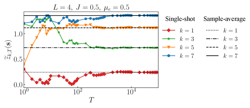
In this paper, hence, we only look at a typical single trajectory and consider the temporal average of quantities after the Lyapunov spectrum becomes stationary when we perform Lyapunov analysis, unless otherwise mentioned. Specifically, we determine the time at which the Lyapunov spectrum is sufficiently stationary, on the basis of the following criteria. First, we evolve the circuit and compute for all at each time after . Then, we compute the averages and the standard deviations of over the last steps, and if the ratios of the standard deviations to the average are less than for all , we stop the calculation and compute physical quantities averaged over the last steps.
II Bipartite mutual information and topological entanglement entropy
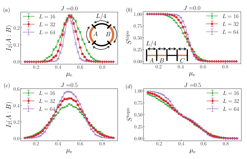
Our model exhibits a phase transition from the topological area-law phase to the trivial area-law phase as increases, when the unitary dynamics is absent. In the presence of the unitary dynamics, the phase transitions occur twice: One is the transition from the topological area-law phase to the critical phase, and the other is the transition from the critical phase to the trivial area-law phase. To confirm this, we first examine the behaviors of conventionally studied quantities, i.e., the bipartite mutual information and topological entanglement entropy (see, e.g., [26, 39, 42]). The bipartite mutual information between subsystems and is given by
| (S26) |
We study for the circuits with PBC and consider the partition of the system as shown in Fig. S2(a). Next, the topological entanglement entropy is defined by [73]
| (S27) |
for the circuits with OBC and for the partition of the system as shown in Fig. S2(b). Note that in the above expressions represents the von Neumann entanglement entropy of a subsystem , which can be computed from the correlation matrix in the following way. We first construct a submatrix by extracting only the space corresponding to the subsystem from the original correlation matrix with . From its eigenvalues with , we can obtain the von Neumann entanglement entropy by
| (S28) |
We now argue that at a phase transition point described by (1+1)-dimensional conformal field theory (CFT), both bipartite mutual information and topological entanglement entropy take constant values independent of the system size, provided that the ratio of the partitions of the system is fixed. This indicates that the transition point can be estimated from the point at which and computed for different system sizes collapse into a single point. For the bipartite mutual information , we consider a one-dimensional chain of the length with PBC, which corresponds to an infinite cylinder with the circumference in the space-time complex coordinate system. Given the partition and , we need to evaluate the following quantity [74, 75],
| (S29) |
where is the reduced density matrix for the subsystem , is the twist field of the conformal dimension , and with . After the conformal mapping onto the infinite complex plane, we can evaluate -point correlation functions of the twist fields in r.h.s of Eq. (S29) from global conformal invariance and find
| (S30) |
which is a function of the cross ratio defined by
| (S31) |
We note that and used here are not related to and used for Lyapunov analysis. For the partition of the system into four segments of the equal length , the cross ratio is independent of the system size (), and so is the bipartite mutual information , which can be computed from the limit of the logarithm of Eq. (S30).
For the topological entanglement entropy , we consider a one-dimensional chain of the length with OBC, which corresponds to an infinite strip of the width . Given the partition , , and , we need to evaluate
| (S32) |
After the conformal mapping onto the upper half plane, the -point correlation functions of the twist field in r.h.s can be evaluated in the infinite complex plane via the method of images [76], which yields
| (S33) |
Since this involves a six-point function of , global conformal invariance dictates that it should be a function of three cross ratios constructed out of [74],
| (S34) |
where
| (S35) | ||||
| (S36) | ||||
| (S37) |
For the partition of the system into four segments of the equal length , the cross ratios become and . Since they are independent of the system size , the topological entanglement entropy obtained by the logarithm of Eq. (S34) is also independent of .
Now, let us investigate our monitored circuits. We show that the behaviors of the bipartite mutual information and topological entanglement entropy for our circuits are consistent with those for the CFT described above. In Fig. S2(a) and (b), we plot the bipartite mutual information and topological entanglement entropy for the measurement-only circuit with for and , respectively. The bipartite mutual information shows a broad peak in the vicinity of , and the values of the curves of different system sizes at are close. The topological entanglement entropy shows a clear crossing in the vicinity of . These results imply that the topological transition occurs at .
In Fig. S2(c) and (d), we plot and for the circuit with unitary dynamics for and , respectively. Both quantities appear to show two scale-invariant points at and , indicating the entanglement transitions between the topological/trivial area-law phase and the critical phase. While the crossing points of drift as the system size increases due to the large finite size effect, different curves of clearly collapse to a single point at and . From these data, we have roughly determined the location of the entanglement transitions as and . Note that Ref. [51] argued that the phase transitions between the area-law phases and critical phase for weakly monitored Majorana fermions are described by a scale-invariant theory, which is also consistent with our results.
III Lyapunov gap and dynamics of topological invariant
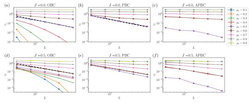
In this section, we first study the scaling form of the lowest non-negative single-particle Lyapunov spectrum with respect to system sizes . The is particularly important because it corresponds to the lowest energy gap of the many-body effective Hamiltonian for large .
In Fig. S3(a,d), we show against , and in the monitored circuit under the OBC with (a) and (d) . In the measurement-only case (), shows a decay faster than the power law in the topological phase (, while it flows towards a finite value in the trivial area-law phase. These results are similar in the presence of unitary dynamics () as well, while appears to decay slowly even in the trivial area-law phase for our available system sizes. At the topological transition ( in the measurement-only circuit, shows a power-law decay with its exponent close to . We can see a similar behavior in the circuit with unitary evolution, while we cannot conclude the true scaling form especially inside the critical phase (.
Next, the spectrum in the monitored circuit under the PBC with and are plotted in Fig. S3(b) and (e), respectively. In the main text, we have discussed the relaxation time of the topological invariant . As corresponds to the many-body gap of the effective Hamiltonian, it characterizes the timescale of the relaxation, i.e., . Here, we can see that scales as near the phase boundaries, while it shows a decay slightly faster than inside the critical phase, leading to at the transition points and inside the critical phase. On the other hand, as decays slower than (or does not decay with respect to ) in the topological and trivial area-law phases, we can conclude . These features can also be seen in the monitored circuit under the APBC except for , as shown in Fig. S3(c,f).
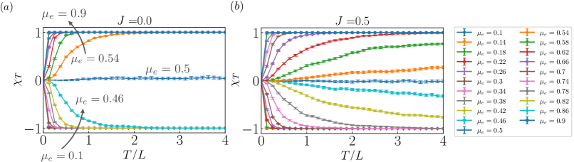
The above argument on the timescale is numerically confirmed by the time series of the topological invariant in the circuits with and as shown in Fig. S4(a) and (b), respectively. In the measurement-only circuit, as for the PBC and APBC become finite except for , rapidly converges to for . On the other hand, in the circuit with , rapidly converges to for in the area-law phases with or , where shows a decay slower than (or no decay), while it takes much longer time to converge inside the critical phase.
Finally, let us discuss . For both cases with and , Fig. S3(c,f) shows that at is about ten times smaller than those at the other . This implies that there exists an exact gap closing in the APBC circuit near . Because of the small , becomes much longer at this point. This leads to the fact that with takes a value close to zero for much longer times than those with the other values of , as shown in Fig. S4.