Topologically protected measurement of orbital angular momentum of light
Abstract
We develop a weak measurement scheme for measuring orbital angular momentum (OAM) of light based on the global topology in wave function. We introduce the spin-orbit coupling to transform the measurement of OAM to the pre- and postselected measurement of polarization. The OAM number can be precisely and promptly recognized using single-shot detection without the need for spatial resolution. More significantly, the measurement results exhibit topological robustness under random phase perturbations. This scheme has the potential to be applied as a paradigm in the OAM-based optical computing, metrology and communication.
The discovery of the quantum Hall effect sparked the insight of studying physical phenomena from a topological perspective Klitzing et al. (1980); Thouless et al. (1982). More profound realm was reached with the advent of topological insulators Kane and Mele (2005); Bernevig and Zhang (2006). The robustness of the edge states is attributed to the nontrivial topological invariant inherent in the energy level structure Hatsugai (1993); Qi and Zhang (2011); Hasan and Kane (2010). By analogy with the solid-state electron system, topology was introduced into photonic crystals to enable a unidirectional and backscattering-immune propagation of electromagnetic fields Wang et al. (2008, 2009). Since then, topological photonic crystals have not only been used to simulate the novel Hall effects in condensed matter Hafezi et al. (2011); Rechtsman et al. (2013); Barik et al. (2018); Shalaev et al. (2019), but also prompted some intriguing applications including topological lasers Bahari et al. (2017); Zeng et al. (2020), topological light funnels Weidemann et al. (2020) and topological antennas Lumer and Engheta (2020).
Topology can also be manifested in the wave function of photon in free space. For a light field paraxially propagating along the -direction, it permits a vortex phase profile that winds around a certain point. Considering a cylindrical coordinate and the presence of rotational symmetry, the wave function can be of the form with denoting the amplitude and the phase Jalali Mehrabad et al. (2023). The periodicity of the wave function implies the identity , which thereby requires that should be an integer. Furthermore, let denote the -component of the orbital angular momentum (OAM) operator and write it as in the coordinate representation Bliokh and Nori (2015). The eigenvalue equation indicates that characterizes the quantum number of OAM. Since the wave functions with different OAM numbers are orthogonal to each other, large-dimensional information can be encoded on single photons, which facilitates a broad range of applications in classical and quantum information Willner et al. (2021); Luo et al. (2015); Yang et al. (2022).
Accordingly, how to realize a precise and rapid measurement of OAM is an essential problem of wide concern. An orthodox method rests on the conversion from OAM beam to Gaussian beam, and then a spatial filter isolates the Gaussian beam to detect Mair et al. (2001); Schlederer et al. (2016). The low efficiency comes from the limited utilization of photons, and possible OAM states necessitating measurements. Other methods, such as interference Huang et al. (2013); Sztul and Alfano (2006); Zhao et al. (2020); Zhang et al. (2014) and diffraction Dai et al. (2015); Kotlyar et al. (2017); Berkhout et al. (2010); Lavery et al. (2012); Hickmann et al. (2010), enable an indirect measurement in the far-field intensity distribution. The requirement of a detector with spatial resolution implies a restricted temporal response. More critically, the aforementioned methodologies are proposed based on light propagation without scattering or turbulence. It has been revealed that when an OAM beam is affected by atmospheric turbulence, the OAM mode will uniformly spread out Paterson (2005); Tyler and Boyd (2009); Rodenburg et al. (2012); Malik et al. (2012); Ren et al. (2013). In this case, the rotational symmetry is broken and the wave function is in the general form , with denoting the phase. The average OAM number is then given by
| (1) |
where denotes a closed loop without self-intersection and is an in-plane vector. Equation. (1) suggests a topological robustness that the average OAM number would remain unchanged even though there is spatial variation in wave function.
In this Letter, we are motivated by the topological protection to propose a scheme for measuring OAM. We employ the spin-orbit coupling to build a weak measurement system Aharonov et al. (1988); Hosten and Kwiat (2008); Dixon et al. (2009); Lundeen et al. (2011); Kocsis et al. (2011); Xu et al. (2013), which permits single-shot detection without the need for spatial resolution. Considerable advantages are manifested in our scheme. The OAM number can be precisely and promptly measured. More significantly, we show that the measurement results can be robust under random phase perturbations.
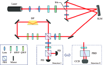
The schematic diagram of our experimental setup is illustrated in Fig. 1. We use a He-Ne laser to emit a Gaussian beam with the wavelength of 633 nm, which is then expanded and collimated by a two-lens telescope to yield a waist of 0.66 mm. A half wave plate (HWP) and a polarizer are combined to adjust the light intensity and lock the polarization direction in the horizontal to match the working axis of the spatial light modulator (SLM). The display screen of SLM with the pixel pitch of 8 µm is divided into left and right parts. We let the laser beam firstly impinge on the left part, where a fork-shaped grating is loaded to transform a Gaussian beam to an array of OAM beams Topuzoski and Janicijevic (2011). Two lenses and an iris make up a spatial filter such that only the first diffraction order is allowed to pass. The filtered OAM beam is redirected to impinge on the right part of SLM, where a time-varying random phase distribution is programmed. Each phase unit is composed of 88 SLM pixels. After diffracting at a distance about 200 mm, the disturbed OAM wave function is generated.
In the weak measurement system, a polarizer is placed with the polarizing direction set to . Two lenses with the focal length of 250 mm establish a 4 imaging system to remove the adverse effect of optical diffraction during the following measurement. We apply a polarizing beam splitter (PBS) to construct a rectangular Sagnac interferometer, wherein the common-path structure in propagating can make measurements robust to external disturbances, such as vibrations and thermal air currents. Through the PBS, the horizontally polarized component is transmitted while the vertically polarized component is reflected. The combination of two quarter wave plates (the fast axes set to ) and a HWP (the fast axis set to ) can introduce a Pancharatnam-Berry (PB) phase of to the horizontal and the vertical polarization states, which are denoted by and , respectively Loredo et al. (2009). The preselected state before the weak coupling is therefore given by
| (2) |
The Dove prism (DP) is rotated by an angle of , such that the wave functions of two orthogonally polarized beams are rotated by an amount of in opposite directions, resulting in the spin-orbit coupling Magaña Loaiza et al. (2014). Assuming that is sufficiently small, we can use a unitary operator to describe the weak coupling and expand it up to the first order, which is written as
| (3) |
where the Pauli spin operator is defined by . The two beams are recombined by emerging from the PBS. We place a HWP (the fast axis set to ) and another PBS to project the photons in the state or . In consideration of the PB phase induced to the state , two exit ports correspond to the postselected states
| (4) |
and
| (5) |
Consequently, the probability distributions are respectively given by
| (6) |
and
| (7) |
where is the abbreviation of . It is not difficult to note that , which implies that we may integrate the difference in probability to obtain the topologically invariant OAM number as suggested by Eq. (1).
In the presence of rotational symmetry, the wave function reads . It follows that . Since a practical detector records results from a statistical accumulation of numerous photons, it would be convenient to define the dimensionless variable termed contrast ratio, which takes the form of
| (8) |
where represents the integral of a function over the entire space, i.e., . In the third line of Eq. (8), the higher-order terms with respect to are neglected. Therefore, we can respectively place two photon detectors behind the two exit ports to measure the light intensities and thereafter calculate the contrast ratio. For the purpose of monitoring beam quality in real time, we can adopt a different strategy. A polarizing beam displacer that can separate the state from the state by 5 mm in space, and a charge coupled device (CCD) are employed.
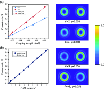
For verification, first consider the case where no random phase is exerted, which means that the right part of SLM is plain. We use a micrometer to fine rotate the DP so as to slightly adjust the coupling strength. The left of Fig. 2(a) shows the contrast ratio with respect to different coupling strengths (=0.021, 0.056, 0.072, and 0.101 rad). is linearly proportional to and the slope is greater for a larger OAM number. The right shows the normalized intensity distributions detected by CCD, giving a visualized contrast between and as increasing. In Fig. 2(b), the values of with and ranging from to 4 are measured. It indicates that the contrast ratio is a good pointer for OAM. The intensity distributions when are also illustrated, which confirms that is greater than for a positive OAM number, whereas the relation is reversed as the sign of OAM is changed. Therefore, our scheme enables a flexible strategy in practical measurement. If the possible value of OAM is in a wide range, we should make the coupling strength small enough to include all the possibilities. If certain OAM numbers suffice to information transmission but the requirement for measurement accuracy is critical, we can increase the coupling strength to achieve a high contrast, instead.
In the case of a random phase disturbance, the rotational symmetry in wave function is broken. Assume that the randomness is not strong and the random phase can amount to a modulation . The wave function is derived by diffraction at a distance. Under this circumstance, we may decompose the amplitude into and the phase into , with and denoting two linear operators. Disposing of the higher order terms of and making use of the topological invariance, the contrast ratio is thus given by
| (9) |
where we have neglected the dependency on coordinates for brevity. If there is no random phase, say , Eq. (9) will be reduced to Eq. (8). As the value of grows, becomes smaller in that and are both non-negative. In a more quantitative way, we can define to describe the degree of randomness, which means the phase modulation of each unit takes value randomly in the range between 0 and . The second term in the third line of Eq. (9) can be roughly considered of the order of . Consequently, would be quadratically proportional to :
| (10) |
A threefold protection for OAM measurement is manifested in this relation. First, the deviation is cubically dependent on , indicating that a weaker coupling is better at suppressing the random phase disturbance (see Supplemental Material). The second protective effect comes from OAM itself. Light field with a lower OAM number can be more robust against disturbance. The quadratic dependence on benefits from the topological invariance, showing that a near-zero randomness of disturbance can only lead to an insignificant degradation.
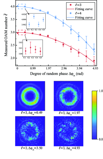
In the experiment, we realize the phase disturbance by loading a random grayscale pattern onto the SLM. Each grayscale unit is associated with a random phase modulation between 0 and . We set the coupling strength to rad and divide by to indicate the measured OAM number. Respectively letting the OAM beams of and enter the weak measurement system, the measured under different are plotted in Fig. 3. It can be found that is reduced as grows, and a larger corresponds to a higher reduction rate. The error bar is initially covered by data symbols when is small, and later is lengthened with increasing. The insets show the detail that the measured is nearly constant in the vicinity of zero randomness. More specifically, the fitting curves for and are drawn based on the functions and . The quadratic coefficient of is greater than that of , which is in agreement with the prediction given by Eq. (10). The increasing of results in a leakage of the measured to a lower OAM number, i.e., crosstalk in measurement emerges. The bottom half of Fig. 3 provides a visual perception of beam quality under different degrees of randomness, which shows that the vortex structure would be hardly recognized when the randomness is severe. Nevertheless, the contrast ratio can partly tell the differences so long as an OAM is carried.
Finally, we have a further discussion of crosstalk. Channel capacity indicates the highest rate that can be achieved in information transmission Shannon (1948). It is formally given by the maximum of the mutual information between the input and output of a channel Cover (1999). In optical communication, if a photon can be in one of input states and its state can be measured without error in the output, the channel capacity reaches the theoretical maximum of . The reduction of channel capacity suggests the emergence of crosstalk.
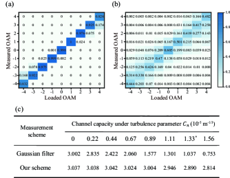
By numerically simulating the transmission of the OAM states from to under atmospheric turbulence Lukin et al. (2012), we compare the channel capacity between the measurement scheme nominated as Gaussian filtering and the measurement scheme proposed by us. Gaussian filtering is widely used in the OAM detection, the principle of which is to transform an OAM beam back to a Gaussian beam by a conjugate phase modulation and then filter the Gaussian beam to detect its intensity Mair et al. (2001); Schlederer et al. (2016). The parameter characterizes the strength of turbulence or, equivalently, the degree of randomness. We adjust the simulation parameters so that the two schemes have nearly the same channel capacity in the absence of turbulence. Figure. 4(a) and (b) present the confusion matrices respectively obtained in our scheme and Gaussian filtering when . Crosstalk is explicitly manifested in the confusion matrix. It can be noted that the measured OAM would leak evenly into the neighboring values for Gaussian filtering. While in our scheme, the contrast ratio only leads to a leakage towards a lower OAM number. The channel capacity with changing from 0 to is tabulated in Fig. 4(c). The channel capacity dramatically decreases for Gaussian filtering. But in our scheme, the channel capacity is stable when is not too large. The topological protection is again manifested.
There is thus a trick if the contrast ratio is applied to recognize the OAM numbers. Since phase disturbance can always make the contrast ratio reduced, we may use the ceiling function to correct the OAM number when the crosstalk is not too severe. But this trick would be invalid in the case where a superposition state of OAM is input. Nevertheless, by combining with methods of demultiplexing Leach et al. (2002), our scheme is also possible to be applied in the sorting of OAM.
In conclusion, we have developed a weak measurement scheme to achieve a topologically protected measurement of OAM of light. We considered random phase distributions as disturbances impacted on the wave function. The quadratical dependence of the measured OAM on the degree of randomness showed a topological robustness. Moreover, single-shot detection without spatial resolution sufficed in our scheme, facilitating a precise and rapid measurement in practical. This work is promising to set a paradigm for OAM measurement in the applications of optical computing, metrology and communication.
Acknowledgements.
This work is supported by the Science Specialty Program of Sichuan University (Grant No.2020SCUNL210).References
- Klitzing et al. (1980) K. v. Klitzing, G. Dorda, and M. Pepper, Phys. Rev. Lett. 45, 494 (1980).
- Thouless et al. (1982) D. J. Thouless, M. Kohmoto, M. P. Nightingale, and M. den Nijs, Phys. Rev. Lett. 49, 405 (1982).
- Kane and Mele (2005) C. L. Kane and E. J. Mele, Phys. Rev. Lett. 95, 226801 (2005).
- Bernevig and Zhang (2006) B. A. Bernevig and S.-C. Zhang, Phys. Rev. Lett. 96, 106802 (2006).
- Hatsugai (1993) Y. Hatsugai, Phys. Rev. Lett. 71, 3697 (1993).
- Qi and Zhang (2011) X.-L. Qi and S.-C. Zhang, Rev. Mod. Phys. 83, 1057 (2011).
- Hasan and Kane (2010) M. Z. Hasan and C. L. Kane, Rev. Mod. Phys. 82, 3045 (2010).
- Wang et al. (2008) Z. Wang, Y. D. Chong, J. D. Joannopoulos, and M. Soljačić, Phys. Rev. Lett. 100, 013905 (2008).
- Wang et al. (2009) Z. Wang, Y. Chong, J. D. Joannopoulos, and M. Soljačić, Nature 461, 772 (2009).
- Hafezi et al. (2011) M. Hafezi, E. A. Demler, M. D. Lukin, and J. M. Taylor, Nature Physics 7, 907 (2011).
- Rechtsman et al. (2013) M. C. Rechtsman, J. M. Zeuner, Y. Plotnik, Y. Lumer, D. Podolsky, F. Dreisow, S. Nolte, M. Segev, and A. Szameit, Nature 496, 196 (2013).
- Barik et al. (2018) S. Barik, A. Karasahin, C. Flower, T. Cai, H. Miyake, W. DeGottardi, M. Hafezi, and E. Waks, Science 359, 666 (2018).
- Shalaev et al. (2019) M. I. Shalaev, W. Walasik, A. Tsukernik, Y. Xu, and N. M. Litchinitser, Nature nanotechnology 14, 31 (2019).
- Bahari et al. (2017) B. Bahari, A. Ndao, F. Vallini, A. E. Amili, Y. Fainman, and B. Kanté, Science 358, 636 (2017).
- Zeng et al. (2020) Y. Zeng, U. Chattopadhyay, B. Zhu, B. Qiang, J. Li, Y. Jin, L. Li, A. G. Davies, E. H. Linfield, B. Zhang, et al., Nature 578, 246 (2020).
- Weidemann et al. (2020) S. Weidemann, M. Kremer, T. Helbig, T. Hofmann, A. Stegmaier, M. Greiter, R. Thomale, and A. Szameit, Science 368, 311 (2020).
- Lumer and Engheta (2020) Y. Lumer and N. Engheta, ACS Photonics 7, 2244 (2020).
- Jalali Mehrabad et al. (2023) M. Jalali Mehrabad, S. Mittal, and M. Hafezi, Phys. Rev. A 108, 040101 (2023).
- Bliokh and Nori (2015) K. Y. Bliokh and F. Nori, Physics Reports 592, 1 (2015), transverse and longitudinal angular momenta of light.
- Willner et al. (2021) A. E. Willner, K. Pang, H. Song, K. Zou, and H. Zhou, Applied Physics Reviews 8, 041312 (2021).
- Luo et al. (2015) X.-W. Luo, X. Zhou, C.-F. Li, J.-S. Xu, G.-C. Guo, and Z.-W. Zhou, Nature communications 6, 7704 (2015).
- Yang et al. (2022) M. Yang, H.-Q. Zhang, Y.-W. Liao, Z.-H. Liu, Z.-W. Zhou, X.-X. Zhou, J.-S. Xu, Y.-J. Han, C.-F. Li, and G.-C. Guo, Nature Communications 13, 2040 (2022).
- Mair et al. (2001) A. Mair, A. Vaziri, G. Weihs, and A. Zeilinger, Nature 412, 313 (2001).
- Schlederer et al. (2016) F. Schlederer, M. Krenn, R. Fickler, M. Malik, and A. Zeilinger, New Journal of Physics 18, 043019 (2016).
- Huang et al. (2013) H. Huang, Y. Ren, Y. Yan, N. Ahmed, Y. Yue, A. Bozovich, B. I. Erkmen, K. Birnbaum, S. Dolinar, M. Tur, and A. E. Willner, Opt. Lett. 38, 2348 (2013).
- Sztul and Alfano (2006) H. I. Sztul and R. R. Alfano, Opt. Lett. 31, 999 (2006).
- Zhao et al. (2020) Q. Zhao, M. Dong, Y. Bai, and Y. Yang, Photon. Res. 8, 745 (2020).
- Zhang et al. (2014) W. Zhang, Q. Qi, J. Zhou, and L. Chen, Phys. Rev. Lett. 112, 153601 (2014).
- Dai et al. (2015) K. Dai, C. Gao, L. Zhong, Q. Na, and Q. Wang, Opt. Lett. 40, 562 (2015).
- Kotlyar et al. (2017) V. V. Kotlyar, A. A. Kovalev, and A. P. Porfirev, Appl. Opt. 56, 4095 (2017).
- Berkhout et al. (2010) G. C. G. Berkhout, M. P. J. Lavery, J. Courtial, M. W. Beijersbergen, and M. J. Padgett, Phys. Rev. Lett. 105, 153601 (2010).
- Lavery et al. (2012) M. P. J. Lavery, D. J. Robertson, G. C. G. Berkhout, G. D. Love, M. J. Padgett, and J. Courtial, Opt. Express 20, 2110 (2012).
- Hickmann et al. (2010) J. M. Hickmann, E. J. S. Fonseca, W. C. Soares, and S. Chávez-Cerda, Phys. Rev. Lett. 105, 053904 (2010).
- Paterson (2005) C. Paterson, Phys. Rev. Lett. 94, 153901 (2005).
- Tyler and Boyd (2009) G. A. Tyler and R. W. Boyd, Opt. Lett. 34, 142 (2009).
- Rodenburg et al. (2012) B. Rodenburg, M. P. J. Lavery, M. Malik, M. N. O’Sullivan, M. Mirhosseini, D. J. Robertson, M. Padgett, and R. W. Boyd, Opt. Lett. 37, 3735 (2012).
- Malik et al. (2012) M. Malik, M. O’Sullivan, B. Rodenburg, M. Mirhosseini, J. Leach, M. P. J. Lavery, M. J. Padgett, and R. W. Boyd, Opt. Express 20, 13195 (2012).
- Ren et al. (2013) Y. Ren, H. Huang, G. Xie, N. Ahmed, Y. Yan, B. I. Erkmen, N. Chandrasekaran, M. P. J. Lavery, N. K. Steinhoff, M. Tur, S. Dolinar, M. Neifeld, M. J. Padgett, R. W. Boyd, J. H. Shapiro, and A. E. Willner, Opt. Lett. 38, 4062 (2013).
- Aharonov et al. (1988) Y. Aharonov, D. Z. Albert, and L. Vaidman, Phys. Rev. Lett. 60, 1351 (1988).
- Hosten and Kwiat (2008) O. Hosten and P. Kwiat, Science 319, 787 (2008).
- Dixon et al. (2009) P. B. Dixon, D. J. Starling, A. N. Jordan, and J. C. Howell, Phys. Rev. Lett. 102, 173601 (2009).
- Lundeen et al. (2011) J. S. Lundeen, B. Sutherland, A. Patel, C. Stewart, and C. Bamber, Nature 474, 188 (2011).
- Kocsis et al. (2011) S. Kocsis, B. Braverman, S. Ravets, M. J. Stevens, R. P. Mirin, L. K. Shalm, and A. M. Steinberg, Science 332, 1170 (2011).
- Xu et al. (2013) X.-Y. Xu, Y. Kedem, K. Sun, L. Vaidman, C.-F. Li, and G.-C. Guo, Phys. Rev. Lett. 111, 033604 (2013).
- Topuzoski and Janicijevic (2011) S. Topuzoski and L. Janicijevic, Journal of Modern Optics 58, 138 (2011).
- Loredo et al. (2009) J. C. Loredo, O. Ortíz, R. Weingärtner, and F. De Zela, Phys. Rev. A 80, 012113 (2009).
- Magaña Loaiza et al. (2014) O. S. Magaña Loaiza, M. Mirhosseini, B. Rodenburg, and R. W. Boyd, Phys. Rev. Lett. 112, 200401 (2014).
- Shannon (1948) C. E. Shannon, The Bell System Technical Journal 27, 379 (1948).
- Cover (1999) T. M. Cover, Elements of information theory (John Wiley & Sons, 1999).
- Lukin et al. (2012) V. P. Lukin, P. A. Konyaev, and V. A. Sennikov, Appl. Opt. 51, C84 (2012).
- Leach et al. (2002) J. Leach, M. J. Padgett, S. M. Barnett, S. Franke-Arnold, and J. Courtial, Phys. Rev. Lett. 88, 257901 (2002).