Topological Nematic Phase Transition
in Kitaev Magnets Under Applied Magnetic Fields
Abstract
We propose a scenario of realizing the toric code phase, which can be potentially utilized for fault-tolerant quantum computation, in candidate materials of Kitaev magnets. It is demonstrated that four-body interactions among Majorana fermions in the Kitaev spin liquid state, which are induced by applied magnetic fields as well as non-Kitaev-type exchange interactions, trigger a nematic phase transition of Majorana bonds without magnetic orders, accompanying the change of the Chern number from to zero. This gapful spin liquid state with zero Chern number is nothing but the toric code phase. Our result potentially explains the topological nematic transition recently observed in -RuCl3 via heat capacity measurements [O. Tanaka et al., arXiv:2007.06757].
I Introduction
A quantum spin liquid (QSL) is an exotic phase of matter, where spins do not have long-range order even at zero temperature. The Kitaev model Kitaev (2006) is an exactly solvable model of QSLs, which is defined on the honeycomb lattice with bond-dependent Ising interactions. A remarkable feature of the Kitaev model is that the system is described by Majorana fermions interacting with gauge fields, allowing the realization of Abelian and non-Abelian anyons. For almost isotropic bond-dependent Ising interactions, the systems exhibits a chiral QSL phase with non-Abelian anyons, when an applied magnetic field opens an energy gap of Majorana fermions. On the other hand, for highly anisotropic Ising interactions, the toric code phase with Abelian anyons is realized. It is noted that both of these phases can be utilized for topological quantum computation Kitaev (2006, 2003). After the Kitaev’s seminal paper, various phenomena associated with Majorana fermions in Kitaev magnets have been extensively explored Baskaran et al. (2007); Feng et al. (2007); Knolle et al. (2014); Nasu et al. (2015); Hermanns et al. (2015a, b); O’Brien et al. (2016); Song et al. (2016); Nasu et al. (2017a); Udagawa (2018); Yamada et al. (2017a); Yamada (2021); Takikawa and Fujimoto (2019, 2020). Since Jackeli and Khaliullin Jackeli and Khaliullin (2009); Yamaji et al. (2014); Rau et al. (2014); Kim and Kee (2016); Winter et al. (2016); Yamada et al. (2017b) pointed out that isotropic bond-dependent Ising interactions arise in some honeycomb layered materials, the experimental search for candidate materials has been an important subject. Several materials including or transition metal ions with a strong spin-orbit coupling have been proposed for Kitaev magnets, such as Lee et al. (2010); Singh and Gegenwart (2010), - Singh et al. (2012), and -RuCl3 Plumb et al. (2014). -RuCl3 under an applied magnetic field is one of the best candidates for the Kitaev magnet Baek et al. (2017). For this material, a signature of Majorana fermions in the chiral QSL phase is observed via the measurement of the half-integer thermal quantum Hall effect Kasahara et al. (2018); Vinkler-Aviv and Rosch (2018); Ye et al. (2018). Moreover, according to the recent specific heat measurements Tanaka et al. (2020), approximated threefold rotational symmetry of the honeycomb lattice is drastically broken to obviously twofold one at high fields, implying that nematic-type phase transition occurs 111Although the crystal structure of -RuCl3 may be monoclinic rather than trigonal Johnson et al. (2015); Kim and Kee (2016), the field angle dependence of heat capacity observed in -RuCl3 by Tanaka et al. Tanaka et al. (2020) shows the symmetry within error bars for magnetic fields T. This approximated threefold rotational symmetry drastically breaks down to obvious twofold one for strong magnetic fields T, which implies the possibility of nematic phase transition in -RuCl3 Tanaka et al. (2020). Remarkably, the nematic phase transition accompanies the disappearance of the half-quantized thermal Hall effect Kasahara et al. (2018), though experimental results suggest that the system may be still in a QSL phase. To understand these observations, we need another ingredient missing in previous research for Kitaev magnets, which includes various additional spin-spin interactions, such as Heisenberg, , and terms.
In this work, we theoretically discuss the possibility of a nematic phase transition due to many-body interactions among itinerant Majorana fermions in Kitaev magnets. Effects of interactions between Majorana fermions have been extensively studied for Kitaev magnets as well as topological superconductors Stoudenmire et al. (2011); Niu et al. (2012); Thomale et al. (2013); Sticlet et al. (2014); Hermanns et al. (2015b); Rahmani et al. (2015); Affleck et al. (2017); Li and Franz (2018); Wamer and Affleck (2018); Rahmani et al. (2019); Rahmani and Franz (2019); Sannomiya and Katsura (2019); Li et al. (2019); Roy et al. (2020); Tummuru et al. (2021); Vishveshwara and Weld (2020); Sachdev and Ye (1993); Maldacena and Stanford (2016); Rahmani and Franz (2019); Yamada (2020). However, physics arising from Majorana interactions in real Kitaev materials is still elusive. On the other hand, various numerical studies on extended Kitaev model utilizing the spin representation, which effectively include non-perturbative effects of Majorana interactions, have been carried out Chaloupka et al. (2010); Okamoto (2013); Rau et al. (2014); Chaloupka and Khaliullin (2016); Nasu et al. (2017b); Gohlke et al. (2018); Rusnačko et al. (2019); Gordon et al. (2019); Jiang et al. (2019); Kaib et al. (2019); Lee et al. (2020); Gohlke et al. (2020); Liu et al. (2021); Buessen and Kim (2021), and nematicity is discussed in recent studies Nasu et al. (2017b); Gohlke et al. (2018); Lee et al. (2020); Gohlke et al. (2020); Liu et al. (2021). Rich phase diagrams of Kitaev magnets are obtained from these studies based on the spin Hamiltonian, while a further theoretical study is needed to understand the results of the recent specific heat measurements mentioned above, which we believe is from the gapped QSL phase to another QSL phase Tanaka et al. (2020).
To focus on the nature of a QSL phase in Kitaev magnets from a different point of view, we assume the flux-free state in our model. Although the flux-free assumption may be violated by strong additional spin-exchanges like Heisenberg, , and terms, it allows us not only to clarify properties of a QSL phase directly but also to explore topological phase transition mentioned above. Besides, under the flux-free assumption we can combine the mean-field analysis and exact diagonalization, which is impossible in the previous framework of the Majorana mean-field theory (see Refs. Gohlke et al. (2018); Knolle et al. (2018), for example), so that we can study rotational symmetry breaking in the extended Kitaev model from various aspects by computing the Majorana band structure, the Majorana bond order, and the Chern number, which are hard to be handled by the direct treatment of the spin model. Furthermore, the scenario that the Majorana four-body interactions give rise to rotational symmetry breaking is applicable to any flux sectors, which is described by interacting Majorana systems, and thus, it is a good starting point to focus on one flux sector. From now on, we elucidate that the four-body interactions can induce nematic-type Majorana bond ordered phase which is a gapped QSL with zero Chern number, i.e. the toric code phase.
II Model
The Hamiltonian of the pure Kitaev model is expressed as,
| (1) |
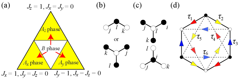
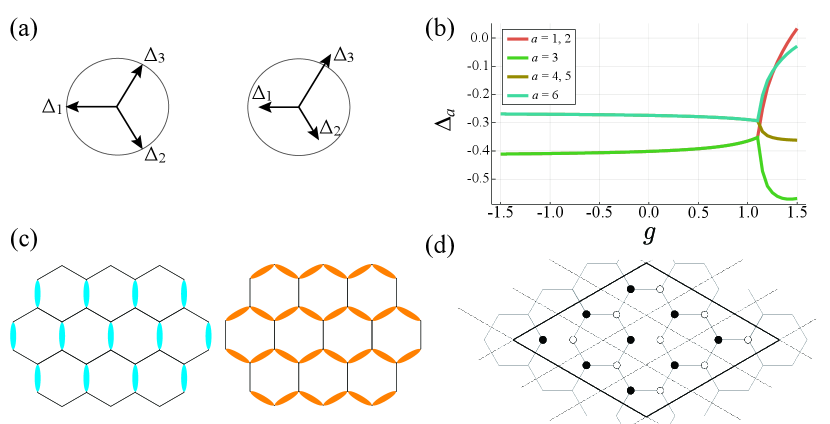
where represents the spin operator on the th site and means a nearest-neighbor (NN) bond. , , and are indices for the bond direction. The phase diagram in the parameter space obtained in Kitaev’s original paper is shown in Fig. 1(a). For strongly anisotropic Kitaev interactions, the so-called phase, which is the toric code phase, is realized. On the other hand, for almost isotropic Kitaev interactions, another phase ( phase), which possesses gapless Dirac bands of Majorana fermions, appears. Once the time-reversal symmetry is broken in phase, however, the spectrum acquires an energy gap, leading to a chiral QSL state with the Chern number . For both phases, the system is described by Majorana fermions interacting with gauge fields. In the following, we restrict our analysis within the vortex-free states. Then, in the case with applied magnetic fields, from the perturbation theory in the third order, effective interactions of three-spin operators are obtained:
| (2) |
where is an external magnetic field and we here assume that . The site summation is taken as shown in Fig. 1(b). In the Majorana representation, operators are rearranged to three types of terms:
| (3) |
where “” means taking the standard gauge in the 0-flux ground state, and means a next-nearest-neighbor (NNN) bond. The first term is an NNN hopping that gives rise to an energy gap, leading to the Chern number , and the others are four-Majorana interactions. Here the site summation for is taken as shown in the upper Y-shaped diagram of Fig. 1(c) and is taken for the lower one of Fig. 1(c). In the following, we focus on these types of Majorana interactions for concreteness. However, we believe that our main results are generic also for other types of neighboring four-body interactions.
It is noted that in the case with the off-diagonal exchange interaction, where run for and , the Y(Y’)-shaped interactions also arise from the third-order perturbation terms of order . Besides, other non-Kitaev interactions, such as Heisenberg and terms, contribute to bring additional NN and NNN hoppings as shown in Appendix C. Thus, generally, the coefficients of the second and the third terms of Eq. (3) are different from that of the first one, and we end up with the following Majorana Hamiltonian,
| (4) |
with
| (5) |
We, here, stress again that the parameters and are independent for real candidate materials of Kitaev magnets, as mentioned above. The Majorana operator is represented as for the th site, and the operators obey and . The hopping amplitude is set unity without loss of generality.
III Mean-field analysis
First, we apply the mean-field (MF) analysis to the four-body interaction term . Then, the general form of the MF Hamiltonian is,
| (6) |
where the index specifies the directions of hopping with the amplitude , as described in Fig. 1(d). The phase factors is necessary to make antisymmetric. The sign of is defined as illustrated in Fig. 1(d) such that the direction of the arrow indicates the positive hopping from the th site to the th site.
Utilizing the Hellmann-Feynman theorem, we can derive self-consistent equations as follows (see Appendix A for more details):
| (7) |
where the definition of bond order parameters is
| (8) |
with being the ground state of the MF Hamiltonian.
We solve the MF Hamiltonian by numerical iteration. First, we focus on a nematic transition. The bond order parameters () play an important role for nematic transitions with rotational symmetry breaking. The Majorana nematic phase considered here is defined as a phase with a bond order in a specific direction. We define nematic order parameters as Pujari et al. (2015),
| (9) |
| (10) |
If (), () must be 0 from the definition, but otherwise will have a nonzero value. In other words, and characterizes breaking of the threefold rotational symmetry.
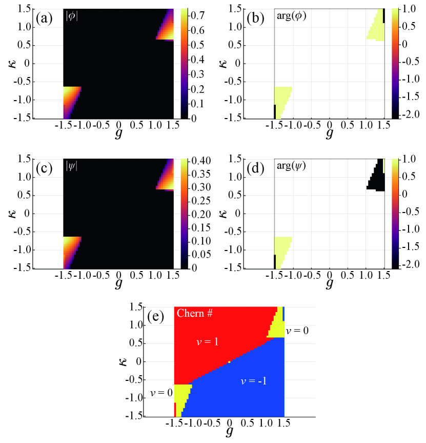
As seen in Figs. 2(a) and (c), for large value of , a nematic phase with , , characterized by two-fold rotational symmetry, appears. We also find in Fig. 2(b) that is in most regions of the area. The argument of has informations about the direction of the nematic order. Since takes a negative value in this calculation, corresponds to the nematic order with . On the other hand, as seen in Fig. 2(d), for in most of the nematic region, while for . This is because that under time-reversal operation, while . In the calculations, we intentionally introduce tiny anisotropy of bonds to obtain symmetry-breaking solutions, lifting three-fold degeneracy.
Now, we examine topological features of the nematic phase. For this purpose, we calculate the Chern number numerically using the Fukui-Hatsugai-Suzuki method Fukui et al. (2005). The results are shown in Fig. 2(e). In the chiral QSL phase without the nematic order, the Chern number . Remarkably, on the other hand, in the nematic phase with and , we find . Thus, the nematic phase transition accompanies the topological phase transition. This implies that the nematic transition which induces strong anisotropy of the Majorana hopping terms (, , in Eq. (6)) drives the system from phase to phase in the phase diagram shown in Fig.1(a). In fact, in this nematic phase, since vortices are still suppressed, the system has no magnetic long-range order, and is in the QSL state. Moreover, the nematic phase is described by the quadratic Hamiltonian of Majorana fermions Eq. (6) with an energy gap. According to Kitaev’s argument on the 16-way of anyons composed of vortices and free fermions Kitaev (2006), the gapful Majorana nematic phase with the Chern number is identified with the toric code phase with Abelian anyons. It is noted that this nematic phase transition is the first-order type with the discontinuous changes of the order parameters and , and hence, there is no gap closing at the transition point. We stress that although the nonzero apparently causes the anisotropy of the Majorana hopping terms, both of the two nematic orders and cooperatively stabilize the toric code phase, since and are nonlinearly coupled with each other via the MF equations. The details are shown in Appendix B.
At the end of this section, we should mention another phase realized in small regions with inside nematic phases shown in Fig.2(e). Although this phase is also a nematic phase with , and hence, is realized. We call this phase “zigzag nematic phase”. This zigzag nematic phase is in phase, i.e. with the Chern number .
IV Exact diagonalization
To confirm the results of the MF calculation, we employ the exact diagonalization calculations. We apply the Lanczos method to the system size up to 32 sites.
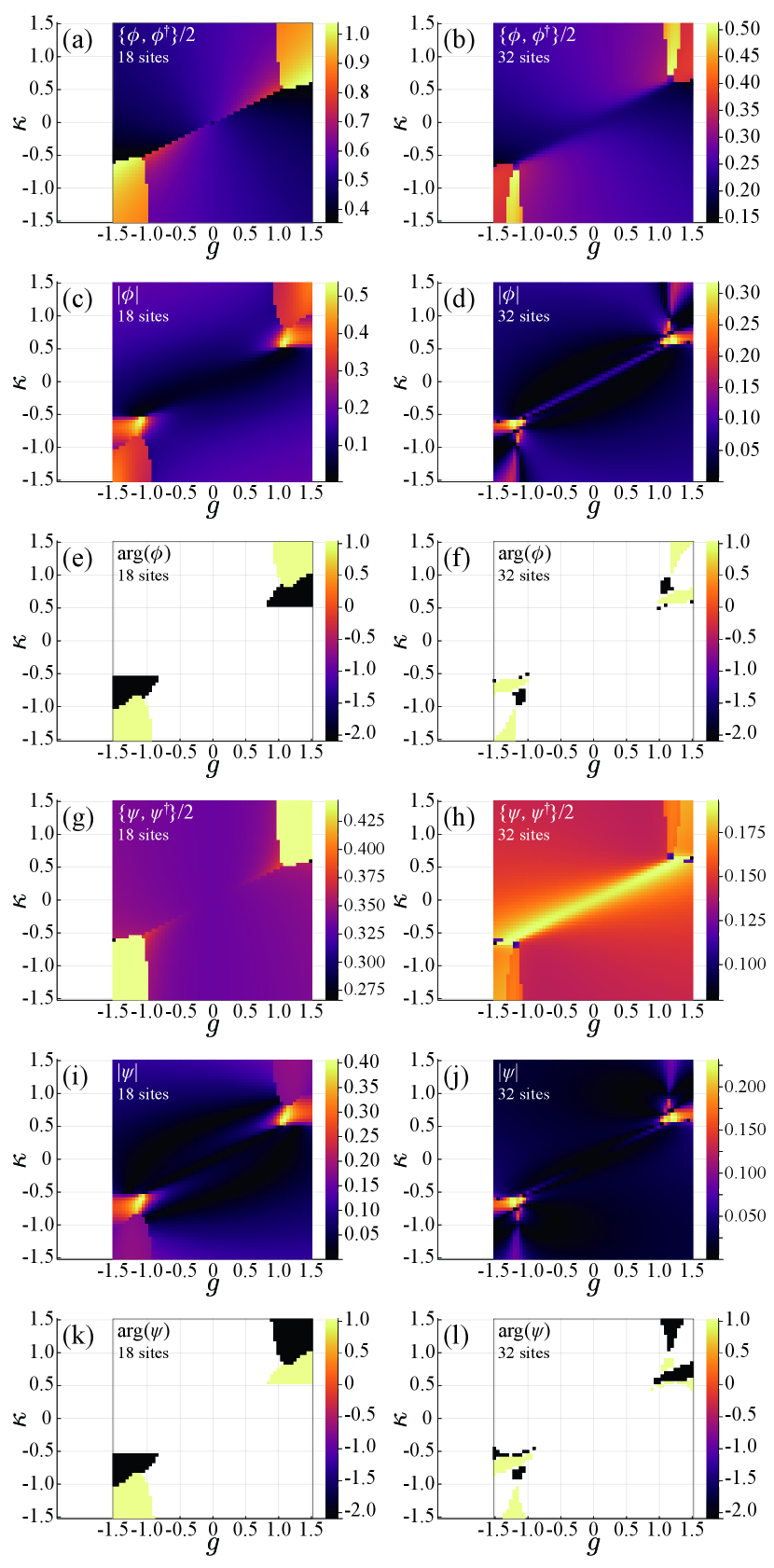
First, we discuss the case of 18 sites. When we use periodic boundary conditions (PBCs), and must be zero, because the system completely preserves the rotational symmetry for finite size systems. Thus, instead, we consider the fluctuation of the order parameters and which can have a nonzero value even for the PBC. The calculated results are shown in Figs. 3(a) and (g). There are two bright yellow regions, which implies that the nematic phase transition occurs discontinuously for large values of . This result confirms the MF calculation. To examine the nematic order more directly, and to determine the direction of bond orders, we switch to an antiperiodic boundary condition (APBC) to intentionally break the threefold rotational symmetry so that we can compute the nonzero and , and the arguments of and . The nematic phase transition is verified again as seen in Figs. 3(c) and (i). Moreover, another phase boundary appears within the nematic regions. This implies that there are two different nematic phases. One is a nematic phase which has one strong bond so that , and the other is a zigzag nematic phase with two strong bonds so that (see Fig. 3(e)). However, the shape of the phase boundary between two nematic phases is quite different from that of the MF result shown in Figs. 2(b) and (d). In fact, this phase boundary crucially depends on the system size, as seen below.
The results of the 32-site calculation are shown in Figs. 3(b), (d), (f), (h), (j), and (l). Although the region of the nematic phase depicted by orange color becomes narrower compared to the 18-site calculation, the nematic phase is definitely realized for large values of . We also find two types of nematic phases as in the MF calculations and the 18-site calculations. However, the shape of the phase boundary is quite different. The region of the zigzag nematic phase with the Chern number , where , (, ) for (), becomes very small for the 32-site calculation. To clarify the fate of the zigzag nematic phase, we need calculations for larger system sizes. Although there is a significant finite-size effect in the calculations, we can clearly observe the tendency towards the nematic phase transition. In the end, small non-zero values in non-nematic phases seen in (c), (d), (i), and (j) are finite-size effects, and decrease toward zero as the system size increases.
V Discussion
Using the MF analysis and the exact diagonalization method, we find that the topological nematic phase transition occurs in strongly correlated regions , . Since non-Kitaev interactions such as off-diagonal exchange interactions significantly renormalize , , and , it is possible to realize this condition for the extended Kitaev model. Particularly, the term reduces the hopping amplitude , and drives the system into strongly correlated regions. We note that the Y(Y’)-shaped interactions of order cancel out for magnetic fields parallel to the honeycomb plane. Nevertheless, other four-body interactions with different configurations of Majorana fermions, which do not disappear even for parallel magnetic fields, can be generated from the Heisenberg exchange interaction and the other off-diagonal exchange interaction, i.e. the term. The details of pertubative calculations with respect to non-Kitaev interactions are shown in Appendix C and we expect that the nematic phase transition recently observed for -RuCl3 under parallel magnetic fields Tanaka et al. (2020) may be explained by taking into account these contributions. To establish this scenario, we need further both theoretical and experimental investigations. It is an interesting future issue to extend our analysis to general flux configurations, for which various Majorana phases are predicted Zhang et al. (2019, 2020). From an experimental side, an electric probe through the hyperfine interaction Yamada and Fujimoto (2020) may be useful for the detection of the Majorana nematic phase.
VI Summary
We have demonstrated that, in the Kitaev spin liquid state, four-body interactions among Majorana fermions which are induced by applied magnetic fields and non-Kitaev exchange interactions give rise to the topological nematic phase transition from the chiral QSL phase to the toric code phase.
Acknowledgements.
We thank Y. Kasahara, Y. Matsuda, and T. Shibauchi for fruitful discussions. This work was supported by JST CREST Grant No. JPMJCR19T5, Japan, and the Grant-in-Aid for Scientific Research on Innovative Areas “Quantum Liquid Crystals (JP20H05163)” from JSPS of Japan, and JSPS KAKENHI (Grant No. JP17K05517, No. JP20K03860 and No. JP20H01857). M.O.T. is supported by Program for Leading Graduate Schools: “Interactive Materials Science Cadet Program”. D.T. is supported by a JSPS Fellowship for Young Scientists and by JSPS KAKENHI Grant No. JP20J20385.Appendix A MEAN-FIELD ANALYSIS AND SELF-CONSISTENT EQUATUIONS
In this section, we reveal the relation between the MF hopping strength and bond order . The Fourier transform of a Majorana operator is given by,
| (11) |
where is the total number of unit cells and represents an each site. is a position type inside the unit cell. In other words, inverse Fourier transform is expressed as
| (12) |
to satisfy and . Using , we can calculate each term of the MF Hamiltonian as,
| (13) | |||||
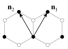
where we choose a basis of the translation group used in Ref. Kitaev (2006) (see Fig. 4).
So the MF Hamiltonian in momentum space is obtained:
| (19) |
where
| (20) |
| (21) | |||||
Then the energy spectrum and the occupied energy under the Fermi level are written as
| (22) |
| (23) |
where the summation is taken over the first Brillouin zone.
Then, we evaluate the mean field energy by using the MF ground state and the MF Hamiltonian ,
| (24) | |||||
where is the total number of sites, and we use,
respectively. Utilizing the Hellmann-Feynman theorem, we obtain,
| (25) |
We can explicitly perform the derivatives using Eq. (23) and get a set of equations,
On the other hand, the total ground state energy which we will take variations with respect to can be easily written as
| (26) |
and one can express the first term and the second term with as
In addition, applying Wick’s theorem, the final term of Eq. (26) can be written as
In short, the total energy density can be expressed as,
| (27) | |||||
Now, we can obtain the self-consistent equations by minimizing the energy with respect to variational parameters ,
| (28) |
or more explicitly,
| (29) |
Finally, comparing Eq. (25) and Eq. (A), we end up with,
| (30) |
Appendix B NEMATIC PHASE AND ZIGZAG NEMATIC PHASE
In this section, we discuss how to distinguish between a nematic phase and a zigzag nematic phase in strongly interacting regions. Since has a negative value in most of parameter regions (see Fig. 5(b)), the nematic order of is schematically expressed as shown in Fig. 5(a); reflects the direction of bond orders with . For instance, implies , which is a direct signal of a nematic phase with one strong bond along the direction. On the other hand, if , there are two strong bonds in directions. In general, represents a nematic phase in a one-strong-bond order and indicates a zigzag nematic phase that has two strong bonds (see Fig. 5(c)). Furthermore, Fig. 5(b) shows that the symmetry breakings of and occur at the same transition point, where we intendedly realize anisotropy of bond orders by substituting several patterns of initial values and take the lowest energy state in each calculation.
We also note symmetrical properties of and under time reversal operation. Since time-reversal operation for Majorana operators depends on the sublattice degrees of freedom, for preserves the time-reversal symmetry, while for changes its sign under time-reversal operation. Therefore, the time-reversal operation acts on and as described below:
| (31) |
Because of these symmetrical properties, is not changed by the transformation and , which correspond to the time-reversal operation, while changes its value as under this transformation, as seen in Figs. 2 and 3 in the main text. In short, for , the region with () corresponds to (), and for , the region with () corresponds to ().
Appendix C DERIVATION OF FOUR-MAJORANA INTERACTIONS ARISING FROM NON-KITAEV INTERACTIONS
In this section, we present the details of the derivation of the four-Majorana interactions caused by non-Kitaev interactions on the basis of perturbative calculations. In these calculations, we need to evaluate matrix elements of perturbation terms for the eigenstates of vortices. For this purpose, we, first, examine the operation of spin operators on the eigenstate, and then, explore for nonzero matrix elements of perturbation terms generated by symmetric off-diagonal exchange interactions, i.e. the term, and the term, and also by the Heisenberg exchange interaction. It is found that the Y-shaped four-Majorana interactions are generated by the term combined with the Zeeman term. On the other hand, the term and the Heisenberg interaction give rise to armchair-shaped interaction, and zigzag-shaped interactions, respectively (see below). Up to the third-order perturbation, this analysis exhausts all four-body interactions among neighboring Majorana fermions generated by the combination of applied magnetic fields and the Heisenberg or the symmetric off-diagonal exchange interactions.
C.1 Flip of gauge fields due to the operation of spin operators
In the following, we use the Majorana representation of spin operators introduced by Kitaev Kitaev (2006), , , . The pure Kitaev model is expressed in terms of itinerant Majorana fields interacting with gauge fields on -bonds (). Here, we consider effects of the operation of spin operators on the eigenstate of flux operators, ,
| (32) | |||||
| (33) | |||||
| (34) |
where and are, respectively, the eigenstates of flux operators, and that of gauge fields , and . We also define a state that is an excited state with a flipped gauge field. Note that the following relations hold:
| (35) | |||||
| (36) | |||||
Using these relations, one can see that is actually a state with a flipped eigenvalue of :
| (37) | |||||
This means that the sign of the eigenvalue of the gauge field for the state is opposite to that of the state. The flip of the gauge field occurs also in the case that the spin operator acts on the other site of the -bond,
| (38) | |||||
| (39) | |||||
C.2 Perturbative calculations with respect to non-Kitaev interactions
We start with the following Hamiltonian for candidate materials of the Kitaev magnet on a honeycomb lattice such as -RuCl3 and Na2IrO3 Rau et al. (2014); Yamaji et al. (2014); Winter et al. (2016); Hou et al. (2017),
| (40) |
| (41) |
| (42) |
| (43) |
| (44) |
where is an component of an spin operator at a site . is the Kitaev interaction, is the Heisenberg exchange interaction between the nearest neighbor sites, and and are symmetric off-diagonal exchange interactions. Here, denotes that the th site and the th site are connected via a nearest-neighbor -bond on the honeycomb lattice. We note that the definitions of , , and are different from conventional ones used in first principle calculations Rau et al. (2014); Winter et al. (2016); Hou et al. (2017) by a factor . We also take into account the Zeeman term due to an external magnetic field ,
| (45) |
Putting , we carry out the perturbative expansions with respect to around the vortex-free ground state in the same spirit as the Kitaev’s paper Kitaev (2006). In this perturbation analysis, intermediate excited states have vortex excitations (visons) with finite energy gaps. On the basis of the results derived in the previous section, we examine nonzero matrix elements in each perturbation term which generates four-Majoarana interactions.
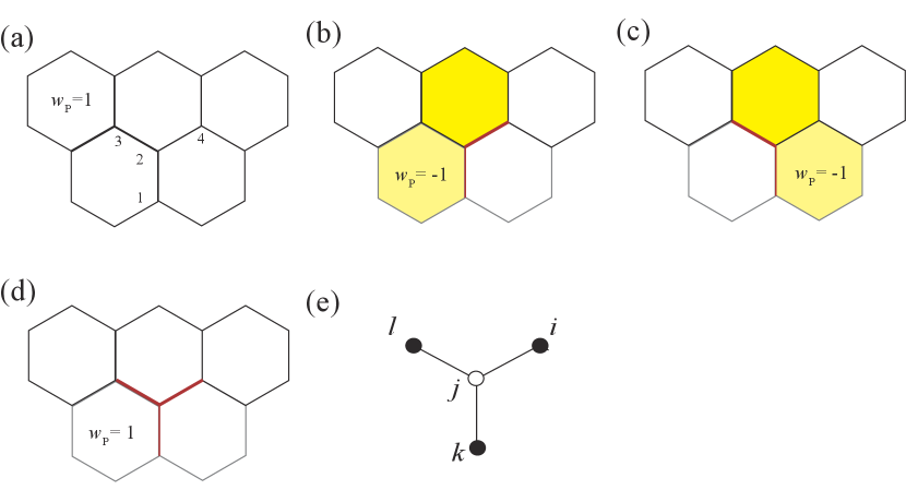
We, first, consider the Y-shaped interaction, which is derived from the third-order perturbation with respect to the term, , and the Zeeman term . To be concrete, we show an example of the perturbation processes in Fig. 6. In this example of the third-order perturbations, the operations of and and on the vortex-free ground state result in the final state, which is also the vortex-free ground state. Thus, these perturbation processes are allowed within the ground state sector. On the other hand, and do not give the perturbation processes within the ground state sector which result in the Y-shaped interaction. Thus, we, here, omit these two terms in . Then, the third-order perturbation term which leads to the Y-shaped interaction is given by,
| (46) | |||||
where , and is a projection to the vortex-free spin liquid state. Also, is the energy gap of two visons, which is given by Kitaev (2006) for the configurations shown in Figs. 6(b), (c). To analyze this term more precisely, we use the fact that in the Majorana fermion representation of the Kitaev spin liquid state, gauge Majorana fields should be paired on the -bond connecting two sites and to form gauge fields , since the Kitaev spin liquid state is expressed by the eigen state of the gauge fields. Then in the case of , Eq. (46) is recast into,
This amounts to the Y-shaped interaction of four itinerant Majorana fermions on the sites , , , shown in Fig. 6(e).
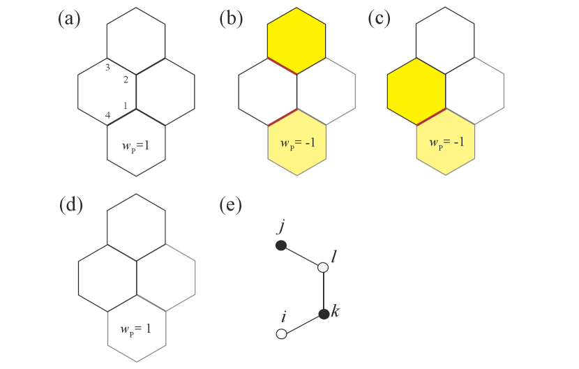
Secondly, we consider the armchair-shaped interaction, which is generated by the third-order perturbation with respect to the term and the Zeeman term. An example of the perturbation processes is shown in Fig. 7. In this example of the third-order perturbations, the operations of and and on the vortex-free ground state generate the final state, which is also the vortex-free ground state. Thus, these perturbation processes are allowed within the ground state sector. On the other hand, and do not generate perturbation processes which lead to the the armchair-shaped interaction satisfying the above condition. Thus, we omit and in in this perturbative calculation. Then, the third-order perturbation term is given by,
| (47) | |||||
where is the energy gap of two visons for the configuration shown in Fig. 7(b) Kitaev (2006). In the Majorana representation, Eq. (47) is recast into,
This results in the armchair-shaped interaction of four neighboring Majorana fermions on the sites , , , shown in Fig. 8(e).
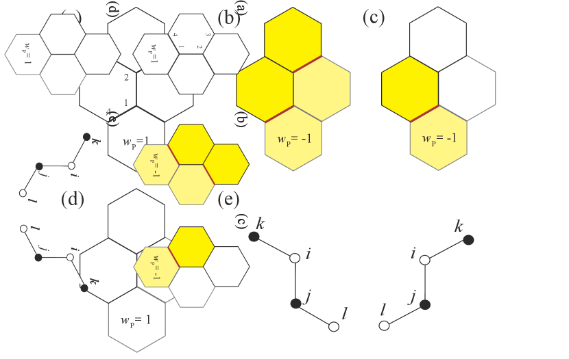
Finally, we consider the zigzag-shaped interaction, which is generated by the third-order perturbation with respect to the Heisenberg term and the Zeeman term . An example of the perturbation processes is shown in Fig. 8. In this example of the third-order perturbations, the operations of and and on the vortex-free ground state generate the final state, which is also the vortex-free ground state. Thus, these perturbation processes are allowed within the ground state sector. On the other hand, and do not contribute to the generation of the zigzag-shaped interaction, and are omitted in the following calculations. Then, the third-order perturbation term is given by,
| (48) | |||||
where represents the energy gap of four visons as illustrated in Fig. 8(b). In the Majorana representation, Eq. (48) is recast into,
This amounts to the zigzag-shaped interaction of four neighboring Majorana fermions on the sites , , , shown in Fig. 8(e).
We, here, stress again that up to the third-order perturbations, the above analysis exhausts all four-body interactions among neighboring Majorana fermions which are generated by the combination of applied magnetic fields and the Heisenberg or symmetric off-diagonal exchange interactions.
We also take into account the renormalization of the nearest-neighbor and next-nearest-neighbor hopping amplitudes of itinerant Majorana fermions due to non-Kitaev interactions and magnetic fields. Then, finally, we obtain the effective Hamiltonian for itinerant Majorana fermions up to the third order perturbation,
| (49) | |||||
where the definitions of the indices of the hopping amplitudes, , are similar to those shown in Fig. 4(b), and means an -bond connecting next-nearest-neighbor sites and , and,
| (50) |
| (51) |
| (52) |
| (53) |
| (54) |
| (55) |
| (56) |
with . In the main text, we put , and to highlight spontaneous rotational-symmetry breaking due to four-Majorana interactions. It is worth mentioning that, as seen in Eqs.(50)-(52), the normalization due to the Heisenberg interaction and the term with , reduces the nearest-neighbor hopping amplitudes in the case of the ferromagnetic Kitaev interaction, . This remarkable feature implies that for real candidate materials such as -RuCl3, where the magnitudes of and are in the same order, the band width of itinerant Majorana fermions is substantially reduced, and thus, the systems may be in strongly correlated regions with in Eq.(5) of the main text, for which the nematic transition occurs.
References
- Kitaev (2006) Alexei Kitaev, “Anyons in an exactly solved model and beyond,” Annals of Physics 321, 2 – 111 (2006), january Special Issue.
- Kitaev (2003) Alexei Kitaev, “Fault-tolerant quantum computation by anyons,” Annals of Physics 303, 2 – 30 (2003).
- Baskaran et al. (2007) G. Baskaran, Saptarshi Mandal, and R. Shankar, “Exact Results for Spin Dynamics and Fractionalization in the Kitaev Model,” Phys. Rev. Lett. 98, 247201 (2007).
- Feng et al. (2007) Xiao-Yong Feng, Guang-Ming Zhang, and Tao Xiang, “Topological Characterization of Quantum Phase Transitions in a Spin- Model,” Phys. Rev. Lett. 98, 087204 (2007).
- Knolle et al. (2014) J. Knolle, D. L. Kovrizhin, J. T. Chalker, and R. Moessner, “Dynamics of a Two-Dimensional Quantum Spin Liquid: Signatures of Emergent Majorana Fermions and Fluxes,” Phys. Rev. Lett. 112, 207203 (2014).
- Nasu et al. (2015) Joji Nasu, Masafumi Udagawa, and Yukitoshi Motome, “Thermal fractionalization of quantum spins in a Kitaev model: Temperature-linear specific heat and coherent transport of Majorana fermions,” Phys. Rev. B 92, 115122 (2015).
- Hermanns et al. (2015a) M. Hermanns, K. O’Brien, and S. Trebst, “Weyl Spin Liquids,” Phys. Rev. Lett. 114, 157202 (2015a).
- Hermanns et al. (2015b) Maria Hermanns, Simon Trebst, and Achim Rosch, “Spin-Peierls Instability of Three-Dimensional Spin Liquids with Majorana Fermi Surfaces,” Phys. Rev. Lett. 115, 177205 (2015b).
- O’Brien et al. (2016) Kevin O’Brien, Maria Hermanns, and Simon Trebst, “Classification of gapless spin liquids in three-dimensional Kitaev models,” Phys. Rev. B 93, 085101 (2016).
- Song et al. (2016) Xue-Yang Song, Yi-Zhuang You, and Leon Balents, “Low-Energy Spin Dynamics of the Honeycomb Spin Liquid Beyond the Kitaev Limit,” Phys. Rev. Lett. 117, 037209 (2016).
- Nasu et al. (2017a) Joji Nasu, Junki Yoshitake, and Yukitoshi Motome, “Thermal Transport in the Kitaev Model,” Phys. Rev. Lett. 119, 127204 (2017a).
- Udagawa (2018) Masafumi Udagawa, “Vison-Majorana complex zero-energy resonance in the Kitaev spin liquid,” Phys. Rev. B 98, 220404 (2018).
- Yamada et al. (2017a) Masahiko G. Yamada, Vatsal Dwivedi, and Maria Hermanns, “Crystalline Kitaev spin liquids,” Phys. Rev. B 96, 155107 (2017a).
- Yamada (2021) Masahiko G. Yamada, “Topological invariant in Kitaev spin liquids: Classification of gapped spin liquids beyond projective symmetry group,” Phys. Rev. Research 3, L012001 (2021).
- Takikawa and Fujimoto (2019) Daichi Takikawa and Satoshi Fujimoto, “Impact of off-diagonal exchange interactions on the Kitaev spin-liquid state of ,” Phys. Rev. B 99, 224409 (2019).
- Takikawa and Fujimoto (2020) Daichi Takikawa and Satoshi Fujimoto, “Topological phase transition to Abelian anyon phases due to off-diagonal exchange interaction in the Kitaev spin liquid state,” Phys. Rev. B 102, 174414 (2020).
- Jackeli and Khaliullin (2009) G. Jackeli and G. Khaliullin, “Mott Insulators in the Strong Spin-Orbit Coupling Limit: From Heisenberg to a Quantum Compass and Kitaev Models,” Phys. Rev. Lett. 102, 017205 (2009).
- Yamaji et al. (2014) Youhei Yamaji, Yusuke Nomura, Moyuru Kurita, Ryotaro Arita, and Masatoshi Imada, “First-Principles Study of the Honeycomb-Lattice Iridates in the Presence of Strong Spin-Orbit Interaction and Electron Correlations,” Phys. Rev. Lett. 113, 107201 (2014).
- Rau et al. (2014) Jeffrey G. Rau, Eric Kin-Ho Lee, and Hae-Young Kee, “Generic Spin Model for the Honeycomb Iridates beyond the Kitaev Limit,” Phys. Rev. Lett. 112, 077204 (2014).
- Kim and Kee (2016) Heung-Sik Kim and Hae-Young Kee, “Crystal structure and magnetism in : An ab initio study,” Phys. Rev. B 93, 155143 (2016).
- Winter et al. (2016) Stephen M. Winter, Ying Li, Harald O. Jeschke, and Roser Valentí, “Challenges in design of Kitaev materials: Magnetic interactions from competing energy scales,” Phys. Rev. B 93, 214431 (2016).
- Yamada et al. (2017b) Masahiko G. Yamada, Hiroyuki Fujita, and Masaki Oshikawa, “Designing Kitaev Spin Liquids in Metal-Organic Frameworks,” Phys. Rev. Lett. 119, 057202 (2017b).
- Lee et al. (2010) Seung-Hun Lee, Hidenori Takagi, Despina Louca, Masaaki Matsuda, Sungdae Ji, Hiroaki Ueda, Yutaka Ueda, Takuro Katsufuji, Jae-Ho Chung, Sungil Park, Sang-Wook Cheong, and Collin Broholm, “Frustrated Magnetism and Cooperative Phase Transitions in Spinels,” Journal of the Physical Society of Japan 79, 011004 (2010).
- Singh and Gegenwart (2010) Yogesh Singh and P. Gegenwart, “Antiferromagnetic Mott insulating state in single crystals of the honeycomb lattice material ,” Phys. Rev. B 82, 064412 (2010).
- Singh et al. (2012) Yogesh Singh, S. Manni, J. Reuther, T. Berlijn, R. Thomale, W. Ku, S. Trebst, and P. Gegenwart, “Relevance of the Heisenberg-Kitaev Model for the Honeycomb Lattice Iridates ,” Phys. Rev. Lett. 108, 127203 (2012).
- Plumb et al. (2014) K. W. Plumb, J. P. Clancy, L. J. Sandilands, V. Vijay Shankar, Y. F. Hu, K. S. Burch, Hae-Young Kee, and Young-June Kim, “: A spin-orbit assisted Mott insulator on a honeycomb lattice,” Phys. Rev. B 90, 041112 (2014).
- Baek et al. (2017) S.-H. Baek, S.-H. Do, K.-Y. Choi, Y. S. Kwon, A. U. B. Wolter, S. Nishimoto, Jeroen van den Brink, and B. Büchner, “Evidence for a Field-Induced Quantum Spin Liquid in -,” Phys. Rev. Lett. 119, 037201 (2017).
- Kasahara et al. (2018) Y. Kasahara, T. Ohnishi, Y. Mizukami, O. Tanaka, Sixiao Ma, K. Sugii, N. Kurita, H. Tanaka, J. Nasu, Y. Motome, T. Shibauchi, and Y. Matsuda, “Majorana quantization and half-integer thermal quantum Hall effect in a Kitaev spin liquid,” Nature 559, 227–231 (2018).
- Vinkler-Aviv and Rosch (2018) Yuval Vinkler-Aviv and Achim Rosch, “Approximately Quantized Thermal Hall Effect of Chiral Liquids Coupled to Phonons,” Phys. Rev. X 8, 031032 (2018).
- Ye et al. (2018) Mengxing Ye, Gábor B. Halász, Lucile Savary, and Leon Balents, “Quantization of the Thermal Hall Conductivity at Small Hall Angles,” Phys. Rev. Lett. 121, 147201 (2018).
- Tanaka et al. (2020) O. Tanaka, Y. Mizukami, R. Harasawa, K. Hashimoto, N. Kurita, H. Tanaka, S. Fujimoto, Y. Matsuda, E. G. Moon, and T. Shibauchi, “Thermodynamic evidence for field-angle dependent Majorana gap in a Kitaev spin liquid,” (2020), arXiv:2007.06757 [cond-mat.str-el] .
- Note (1) Although the crystal structure of -RuCl3 may be monoclinic rather than trigonal Johnson et al. (2015); Kim and Kee (2016), the field angle dependence of heat capacity observed in -RuCl3 by Tanaka et al. Tanaka et al. (2020) shows the symmetry within error bars for magnetic fields T. This approximated threefold rotational symmetry drastically breaks down to obvious twofold one for strong magnetic fields T, which implies the possibility of nematic phase transition in -RuCl3 Tanaka et al. (2020).
- Stoudenmire et al. (2011) E. M. Stoudenmire, Jason Alicea, Oleg A. Starykh, and Matthew P.A. Fisher, “Interaction effects in topological superconducting wires supporting Majorana fermions,” Phys. Rev. B 84, 014503 (2011).
- Niu et al. (2012) Yuezhen Niu, Suk Bum Chung, Chen-Hsuan Hsu, Ipsita Mandal, S. Raghu, and Sudip Chakravarty, “Majorana zero modes in a quantum Ising chain with longer-ranged interactions,” Phys. Rev. B 85, 035110 (2012).
- Thomale et al. (2013) Ronny Thomale, Stephan Rachel, and Peter Schmitteckert, “Tunneling spectra simulation of interacting Majorana wires,” Phys. Rev. B 88, 161103 (2013).
- Sticlet et al. (2014) Doru Sticlet, Luis Seabra, Frank Pollmann, and Jérôme Cayssol, “From fractionally charged solitons to Majorana bound states in a one-dimensional interacting model,” Phys. Rev. B 89, 115430 (2014).
- Rahmani et al. (2015) Armin Rahmani, Xiaoyu Zhu, Marcel Franz, and Ian Affleck, “Phase diagram of the interacting Majorana chain model,” Phys. Rev. B 92, 235123 (2015).
- Affleck et al. (2017) Ian Affleck, Armin Rahmani, and Dmitry Pikulin, “Majorana-Hubbard model on the square lattice,” Phys. Rev. B 96, 125121 (2017).
- Li and Franz (2018) Chengshu Li and Marcel Franz, “Majorana-Hubbard model on the honeycomb lattice,” Phys. Rev. B 98, 115123 (2018).
- Wamer and Affleck (2018) Kyle Wamer and Ian Affleck, “Renormalization group analysis of phase transitions in the two-dimensional Majorana-Hubbard model,” Phys. Rev. B 98, 245120 (2018).
- Rahmani et al. (2019) Armin Rahmani, Dmitry Pikulin, and Ian Affleck, “Phase diagrams of Majorana-Hubbard ladders,” Phys. Rev. B 99, 085110 (2019).
- Rahmani and Franz (2019) Armin Rahmani and Marcel Franz, “Interacting Majorana fermions,” Reports on Progress in Physics 82, 084501 (2019).
- Sannomiya and Katsura (2019) Noriaki Sannomiya and Hosho Katsura, “Supersymmetry breaking and Nambu-Goldstone fermions in interacting Majorana chains,” Phys. Rev. D 99, 045002 (2019).
- Li et al. (2019) Chengshu Li, Étienne Lantagne-Hurtubise, and Marcel Franz, “Supersymmetry in an interacting Majorana model on the kagome lattice,” Phys. Rev. B 100, 195146 (2019).
- Roy et al. (2020) Ananda Roy, Johannes Hauschild, and Frank Pollmann, “Quantum phases of a one-dimensional Majorana-Bose-Hubbard model,” Phys. Rev. B 101, 075419 (2020).
- Tummuru et al. (2021) Tarun Tummuru, Alberto Nocera, and Ian Affleck, “Triangular lattice Majorana-Hubbard model: Mean-field theory and DMRG on a width-4 torus,” Phys. Rev. B 103, 115128 (2021).
- Vishveshwara and Weld (2020) Smitha Vishveshwara and David M. Weld, “ phases and Majorana spectroscopy in paired Bose-Hubbard chains,” (2020), arXiv:2012.02380 [cond-mat.quant-gas] .
- Sachdev and Ye (1993) Subir Sachdev and Jinwu Ye, “Gapless spin-fluid ground state in a random quantum Heisenberg magnet,” Phys. Rev. Lett. 70, 3339–3342 (1993).
- Maldacena and Stanford (2016) Juan Maldacena and Douglas Stanford, “Remarks on the Sachdev-Ye-Kitaev model,” Phys. Rev. D 94, 106002 (2016).
- Yamada (2020) Masahiko G. Yamada, “Anderson-Kitaev spin liquid,” npj Quantum Mater. 5, 82 (2020).
- Chaloupka et al. (2010) Ji ří Chaloupka, George Jackeli, and Giniyat Khaliullin, “Kitaev-Heisenberg Model on a Honeycomb Lattice: Possible Exotic Phases in Iridium Oxides ,” Phys. Rev. Lett. 105, 027204 (2010).
- Okamoto (2013) Satoshi Okamoto, “Doped Mott Insulators in (111) Bilayers of Perovskite Transition-Metal Oxides with a Strong Spin-Orbit Coupling,” Phys. Rev. Lett. 110, 066403 (2013).
- Chaloupka and Khaliullin (2016) Ji ří Chaloupka and Giniyat Khaliullin, “Magnetic anisotropy in the Kitaev model systems and ,” Phys. Rev. B 94, 064435 (2016).
- Nasu et al. (2017b) Joji Nasu, Yasuyuki Kato, Junki Yoshitake, Yoshitomo Kamiya, and Yukitoshi Motome, “Spin-Liquid–to–Spin-Liquid Transition in Kitaev Magnets Driven by Fractionalization,” Phys. Rev. Lett. 118, 137203 (2017b).
- Gohlke et al. (2018) Matthias Gohlke, Gideon Wachtel, Youhei Yamaji, Frank Pollmann, and Yong Baek Kim, “Quantum spin liquid signatures in Kitaev-like frustrated magnets,” Phys. Rev. B 97, 075126 (2018).
- Rusnačko et al. (2019) Juraj Rusnačko, Dorota Gotfryd, and Ji ří Chaloupka, “Kitaev-like honeycomb magnets: Global phase behavior and emergent effective models,” Phys. Rev. B 99, 064425 (2019).
- Gordon et al. (2019) Jacob S. Gordon, Andrei Catuneanu, Erik S. Srensen, and Hae-Young Kee, “Theory of the field-revealed Kitaev spin liquid,” Nature Communications 10, 2470 (2019).
- Jiang et al. (2019) Yi-Fan Jiang, Thomas P. Devereaux, and Hong-Chen Jiang, “Field-induced quantum spin liquid in the Kitaev-Heisenberg model and its relation to ,” Phys. Rev. B 100, 165123 (2019).
- Kaib et al. (2019) David A. S. Kaib, Stephen M. Winter, and Roser Valentí, “Kitaev honeycomb models in magnetic fields: Dynamical response and dual models,” Phys. Rev. B 100, 144445 (2019).
- Lee et al. (2020) Hyun-Yong Lee, Ryui Kaneko, Li Ern Chern, Tsuyoshi Okubo, Youhei Yamaji, Naoki Kawashima, and Yong Baek Kim, “Magnetic field induced quantum phases in a tensor network study of Kitaev magnets,” Nature Communications 11 (2020), 10.1038/s41467-020-15320-x.
- Gohlke et al. (2020) Matthias Gohlke, Li Ern Chern, Hae-Young Kee, and Yong Baek Kim, “Emergence of nematic paramagnet via quantum order-by-disorder and pseudo-Goldstone modes in Kitaev magnets,” Phys. Rev. Research 2, 043023 (2020).
- Liu et al. (2021) Ke Liu, Nicolas Sadoune, Nihal Rao, Jonas Greitemann, and Lode Pollet, “Revealing the phase diagram of Kitaev materials by machine learning: Cooperation and competition between spin liquids,” Phys. Rev. Research 3, 023016 (2021).
- Buessen and Kim (2021) Finn Lasse Buessen and Yong Baek Kim, “Functional renormalization group study of the Kitaev- model on the honeycomb lattice and emergent incommensurate magnetic correlations,” Phys. Rev. B 103, 184407 (2021).
- Knolle et al. (2018) Johannes Knolle, Subhro Bhattacharjee, and Roderich Moessner, “Dynamics of a quantum spin liquid beyond integrability: The Kitaev-Heisenberg- model in an augmented parton mean-field theory,” Phys. Rev. B 97, 134432 (2018).
- Pujari et al. (2015) Sumiran Pujari, Fabien Alet, and Kedar Damle, “Transitions to valence-bond solid order in a honeycomb lattice antiferromagnet,” Phys. Rev. B 91, 104411 (2015).
- Fukui et al. (2005) Takahiro Fukui, Yasuhiro Hatsugai, and Hiroshi Suzuki, “Chern Numbers in Discretized Brillouin Zone: Efficient Method of Computing (Spin) Hall Conductances,” Journal of the Physical Society of Japan 74, 1674–1677 (2005), https://doi.org/10.1143/JPSJ.74.1674 .
- Zhang et al. (2019) Shang-Shun Zhang, Zhentao Wang, Gábor B. Halász, and Cristian D. Batista, “Vison Crystals in an Extended Kitaev Model on the Honeycomb Lattice,” Phys. Rev. Lett. 123, 057201 (2019).
- Zhang et al. (2020) Shang-Shun Zhang, Cristian D. Batista, and Gábor B. Halász, “Toward Kitaev’s sixteenfold way in a honeycomb lattice model,” Phys. Rev. Research 2, 023334 (2020).
- Yamada and Fujimoto (2020) Masahiko G. Yamada and Satoshi Fujimoto, “Electric probe for the toric code phase in Kitaev materials through the hyperfine interaction,” (2020), arXiv:2012.08825 [cond-mat.str-el] .
- Hou et al. (2017) Y. S. Hou, H. J. Xiang, and X. G. Gong, “Unveiling magnetic interactions of ruthenium trichloride via constraining direction of orbital moments: Potential routes to realize a quantum spin liquid,” Phys. Rev. B 96, 054410 (2017).
- Johnson et al. (2015) R. D. Johnson, S. C. Williams, A. A. Haghighirad, J. Singleton, V. Zapf, P. Manuel, I. I. Mazin, Y. Li, H. O. Jeschke, R. Valentí, and R. Coldea, “Monoclinic crystal structure of and the zigzag antiferromagnetic ground state,” Phys. Rev. B 92, 235119 (2015).