Topological Magnonic Properties of an Antiferromagnetic Chain

Topojit Debnath [email protected] Laboratory for Terahertz

\&

Terascale Electronics (LATTE), Department of Electrical and Computer Engineering, University of California, Riverside, CA, 92521, USA Shri Hari Soundararaj [email protected] Materials Science and Engineering, University of California, Riverside, CA, 92521, USA Sohee Kwon [email protected] Laboratory for Terahertz

\&

Terascale Electronics (LATTE), Department of Electrical and Computer Engineering, University of California, Riverside, CA, 92521, USA Alexander A. Balandin [email protected] Department of Materials Science and Engineering, University of California, Los Angeles, CA 90095, USA Roger K. Lake [email protected] Laboratory for Terahertz

\&

Terascale Electronics (LATTE), Department of Electrical and Computer Engineering, University of California, Riverside, CA, 92521, USA

Abstract

The magnonic excitations of a dimerized, one-dimensional, antiferromagnetic chain can be trivial or topological depending on the signs and magnitudes of the alternating exchange couplings and the anisotropy. The topological phase that occurs when the signs of the two different exchange couplings alternate is qualitatively different from that of the Su-Schrieffer-Heeger model. A material that may exhibit these properties is the quasi-one-dimensional material MoI₃ that consists of dimerized chains weakly coupled to adjacent chains. The magnetic ground state and its excitations are analyzed both analytically and numerically using exchange and anisotropy parameters extracted from density functional theory calculations.

Quasi-one-dimensional materials, topological magnonics, antiferromagnet

I Introduction

Anti-ferromagnetism and topological magnonics [1, 2, 3, 4] in low-dimensional materials are of high current interest. The majority of the work in topological magnonics has focused on two-dimensional (2D) ferromagnetic (FM) and antiferromagnetic (AFM) systems. The 2D systems generally rely on the presence of the Dzyaloshinskii-Moriya interaction, which serves as an analogue to spin-orbit coupling in electronic systems, to obtain a topological magnonic phase. In one-dimensional electronic systems, dimerization can result in a topological phase described by the Su-Schrieffer-Heeger (SSH) model [5], and in one-dimensional FM systems, dimerization results in a magnetic analogue of the SSH model with a topological magnonic phase [6, 7]. We will show that dimerization alone does not qualitatively alter the magnonic spectrum in an AFM spin chain, and that more is required to obtain a topological magnonic phase.

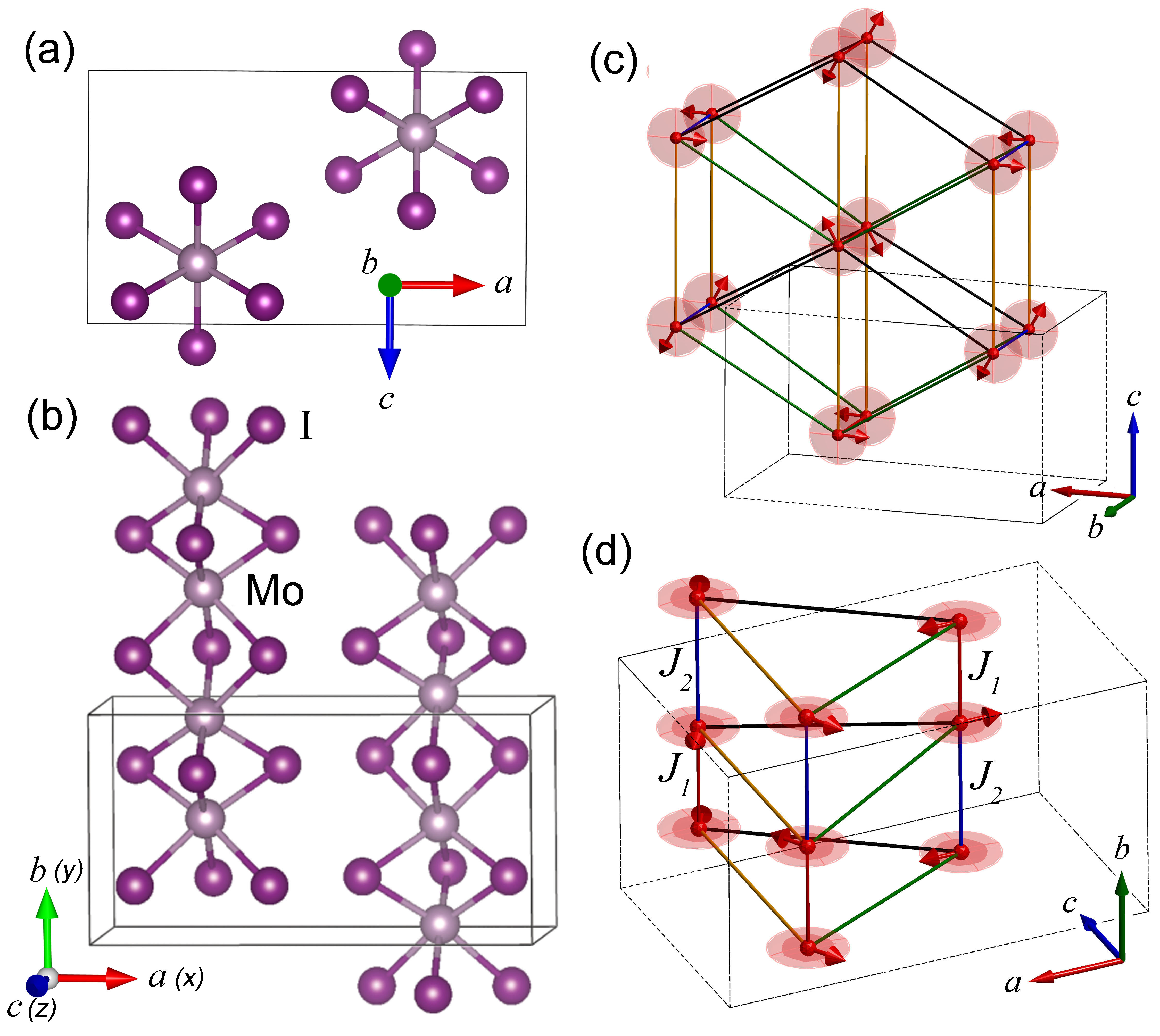
In this paper, we analyze the magnonic properties of a AFM dimerized and tetramerized spin chain. Dimerization causes the AFM exchange coupling between the magnetic atoms along the chain to alternate in magnitude. The two different intrachain exchange couplings, $J_{1}$ and $J_{2}$ , are illustrated in Fig. 1(d). With $J_{1}>J_{2}>0$ (AFM coupling) the magnonic spectrum remains trivial for all positive values of $J_{1}$ and $J_{2}$ . If $J_{2}$ becomes negative, such that the sign of the exchange coupling along the chain alternates, then, depending on the relative magnitudes of $J_{1}$ , $J_{2}$ , and the anisotropy constants, the magnonic spectrum can enter a non-trivial topological state that is qualitatively different from that of the SSH model.

An example quasi-one-dimensional material that may exhibit these magnonic topological properties is the quasi-one-dimensional transition metal tri-halide MoI₃. It consists of covalently bonded MoI₃ chains weakly coupled to adjacent chains in a triangular lattice. The material was recently synthesized and characterized with powder and single-crystal X-ray analysis [8, 9, 10]. The crystal system is orthorhombic with space group Pmmn (59). The chains are dimerized with alternating distances, 2.88 Å and 3.53 Å, between Mo atoms along the chains. There is no known temperature for the chains to transition to the symmetric phase ( $P6_{3}/mmc$ ). Each Mo atom is bonded to 6 I atoms in a distorted octahedral arrangement. A bulk unit cell, doubled along the $b$ axis, is shown from top and side views in Fig. 1(a,b). Bulk samples were characterized by Raman spectroscopy [10]. The temperature variation of several Raman peaks displayed a transition suggestive of a magnetic phase transition. Several peaks that disappeared in the temperature range between 125 - 150 K were considered to originate from two magnon scattering processes. Density functional theory (DFT) calculations found that the lowest energy ground state was easy-plane AFM with alternating spins along the chains. Prior DFT calculations of single chains of transition metal di- and tri-halides also found the ground state of MoI₃ to be AFM [11, 12].

Refer to caption — Figure 1: (a) Top view and (b) side view of two chains that comprise the MoI₃ unit cell. The chains have been doubled along the $b$ axis to show the dimerization. The lattice vector directions, $xyz$ coordinate system, and outline of the unit cell are shown. (c) Relaxed magnetic structure showing only the Mo atoms of a central chain and its six surrounding chains. The circular regions around each spin indicate easy plane anisotropy perpendicular to the axis of the chains. (d) Relaxed magnetic structure illustrating the exchange coupling parameters. Figures are generated by (a,b) Vesta [13] and (c,d) SpinW [14].

Exchange coupling constants and anisotropy energies determined from DFT calculations in Sec. II are used in a Heisenberg type Hamiltonian that is analyzed using linear spin wave theory [15, 16, 17] in the main text and classical effective field theory in the Appendix. Analytical expressions are derived in Sec. III for an individual chain that explicitly show the criteria for transitioning from a topologically trivial to a non-trivial phase. The full magnonic spectrum that includes the interchain coupling is determined numerically in Sec. IV.

II Density Functional Theory Calculations

Density functional theory calculations, as implemented in the Vienna $ab$ $initio$ simulation package (VASP) [18, 19, 20, 21], are performed using the generalized gradient approximation for the exchange-correlation functional as parameterized by Perdew, Burke, and Ernzerhof (PBE) [22]. The van der Waals interaction is included using the PBE-D3 method of Grimme et al. [23]. The energy cutoff for the plane wave basis is 520 eV. Bulk structures are relaxed until the forces on the atoms are smaller than $10^{-4}$ eV/Å. Phonon calculations are performed using the finite-displacement supercell approach as implemented in Phonopy [24, 25] with a $2\times 2\times 2$ supercell, and the Brillouin zone is sampled by a $3\times 6\times 6$ Monkhorst–Pack k-point grid.

Previously, a Hubbard $U$ value of 4 eV was used to prevent the occurrence of negative phonon modes in the phonon dispersion calculations [10]. In this work, we find that by using a tighter convergence criteria during the structure relaxation process, a stable crystal structure can be obtained without including a Hubbard $U$ term. The self consistent field electronic calculations with $U=0$ , $U=2.4$ eV [26], and $U=4$ eV [10] all show the easy-plane AFM spin configuration, with alternating spins along the chains, to be the minimum energy magnetic ground state. However, when the crystal structure is relaxed in the AFM phase, only the $U=0$ calculation results in the dimerized Pmmn ground state. The $U\neq 0$ calculations find the non-dimerized Pmmn phase to be the ground state, which contradicts the experimental results. The total energy difference per unit cell of the dimerized and non-dimerized Pmmn phase (calculated with $U=0$ in the AFM phase) is 0.43 eV. Furthermore, the $U=0$ calculation gives lattice constants (a = 12.41 Å, b =6.45 Å, and c = 7.17 Å) that agree closely with the experimental values [10]. Therefore, all calculations in this work are performed without a Hubbard $U$ correction.

To investigate the inter-chain spin alignment of the charge neutral ground state, we constructed a 1 $\times$ 1 $\times$ 3 supercell and compared the total energies of the non-collinear and collinear AFM states, as shown in Fig. 2. In the collinear configuration, the magnetic moments are aligned along the $\pm a$ axis. In the non-collinear configuration, the magnetic moments of the Mo atoms in the same plane that form the vertices of a triangle are rotated with respect to each other by $120^{\circ}$ as shown in Fig. 2(a). The DFT calculations reveal that the non-collinear AFM state is energetically favored by 14.5 meV compared to the collinear AFM state. This is also the minimum energy state found from the Heisenberg Hamiltonian (1) using exchange parameters extracted from the DFT calculations.

The the magnetic exchange coupling constants and anisotropy energies are determined from the standard energy mapping method [27, 28, 29, 10] with total energies calculated using PBE-D3 with spin-orbit coupling (SOC). The details of the these calculations and an illustration of the interchain exchange parameters, $J_{3}$ and $J_{4}$ , are provided in Appendix A. The results are shown in Table 1.

Filling	Neutral	0.1	0.19	0.196	0.2	0.3	0.4
$J_{1}$	24.08	23.80	23.86	23.88	23.89	24.39	25.42
$J_{2}$	4.44	2.04	0.02	-0.11	-0.20	-2.30	-4.26
$J_{3}$	0.55	0.61	0.67	0.68	0.68	0.74	0.82
$J_{4}$	0.12	0.16	0.19	0.19	0.19	0.21	0.21
$A_{y}$	2.11	2.38	2.57	2.58	2.58	2.76	2.90
$A_{x}$	0	0.12	0.33	0.35	0.36	0.62	0.91

Table 1: Exchange and anisotropy parameters (meV) as a function of hole filling (number of excess holes per unit cell consisting of 4 Mo atoms and 12 I atoms).

In the charge neutral state, all of the exchange coupling parameters are positive (AFM), and the minimum energy spin configuration along the chain, determined from DFT, is illustrated in Fig. 3(a). With $A_{y}=2.11$ meV and $A_{x}=0$ , the spins have easy-plane anisotropy with the easy-plane perpendicular to the chains, as illustrated in Fig. 1(c,d). With hole filling, $J_{2}$ changes sign and the minimum energy spin configuration along the chain switches to that shown in Fig. 3(b). We will refer to this as the magnetically tetramerized unit cell. Furthermore, the in-plane anisotropy $A_{x}$ increases, so that at larger values of hole filling, the ground state spin configuration becomes collinear with all spins aligned along $\pm{\bf c}$ . We analyze the excitations of the magnetic system by first considering the individual chains and then consider the effect of interchain coupling.

III Single Chain Analysis

III.1 Dimerized AFM Single Chain

We begin by analyzing a single chain illustrated in Fig. 3(a) using parameters for the charge neutral state given in Table 1. We do this because the bulk crystal is physically a lattice of weakly coupled chains, and the characteristics of the single chain are still present and visible when interchain coupling is included. Furthermore, the single chain provides a model system to compare against other such model systems found in the literature, falling under the general umbrella of the SSH model. The spin Hamiltonian for this system is

$\displaystyle H$	$\displaystyle=2\sum_{n}\left[J_{1}{\bf S}_{n}^{A}\cdot{\bf S}_{n}^{B}+J_{2}{\bf S}_{n}^{A}\cdot{\bf S}_{n-1}^{B}\right]$	(1)
	$\displaystyle+A_{y}\sum_{n}\left[\left({\bf S}_{n,y}^{A}\right)^{2}+\left({\bf S}_{n,y}^{B}\right)^{2}\right]$
	$\displaystyle+A_{x}\sum_{n}\left[\left({\bf S}_{n,x}^{A}\right)^{2}+\left({\bf S}_{n,x}^{B}\right)^{2}\right].$

In Eq. (1), $J_{1},J_{2}>0$ , i.e. both exchange couplings are antiferromagnetic, and $J_{1}>J_{2}$ . $J_{1}$ is the exchange coupling between the $A$ and $B$ spins within the same unit cell, and $J_{2}$ couples spins between adjacent unit cells. The sum is over unit cells $n$ . $A_{y}\gg A_{x}>0$ are anisotropy terms. $A_{y}$ creates easy-plane anisotropy with the easy plane in the $x$ - $z$ plane perpendicular the axis of the chain. Within the $x$ - $z$ plane a small anisotropy $A_{x}$ is assumed such that the equilibrium spins minimize their energy by aligning and anti-aligning along $z$ .

The magnon excitation spectrum can be calculated using the classical effective field approach or the quantum approach and linear spin wave theory [15, 16, 17]. Here, we will use the quantum approach and linear spin wave theory, and, in Appendix D, we describe the effective field approach. Both approaches result in the same magnon dispersion, however the quantum approach allows for the calculation of the surface Green’s function using the standard decimation algorithm [30, 31, 32].

The analysis begins with the Holstein-Primakoff transformation [33] of the spin operators in Eq. (1). To lowest order in the spin deviation operators,

$\displaystyle\hat{S}_{j,z}^{A}$	$\displaystyle=S-{\hat{n}}^{A}_{j}$
$\displaystyle\hat{S}_{j}^{A+}$	$\displaystyle\approx\sqrt{2S}a_{j}$
$\displaystyle\hat{S}_{j}^{A-}$	$\displaystyle\approx\sqrt{2S}\;{a_{j}^{\dagger}}$	(2)

and

$\displaystyle\hat{S}_{j,z}^{B}$	$\displaystyle=-S+{\hat{n}}^{B}_{j}$
$\displaystyle\hat{S}_{j}^{B+}$	$\displaystyle\approx\sqrt{2S}\;b_{j}^{\dagger}$
$\displaystyle\hat{S}_{j}^{B-}$	$\displaystyle\approx\sqrt{2S}b_{j}$	(3)

where ${\hat{n}}^{A}_{j}={a_{j}^{\dagger}}a_{j}$ , ${\hat{n}}^{B}_{j}=b_{j}^{\dagger}b_{j}$ and $n_{j}\in\{0,1,2,\ldots,2S\}$ so that $S^{A}_{j,z}$ and $S^{B}_{j,z}$ run from $-S$ to $S$ . The creation and annihilation operators follow the usual bosonic commutation relations. Making the above substitutions into Eq. (1), using $S_{x}=\frac{1}{2}\left(S^{+}+S^{-}\right)$ and $S_{y}=\frac{1}{2i}\left(S^{+}-S^{-}\right)$ , and keeping terms up to quadratic order, we have, $H\equiv H_{J_{1}}+H_{J_{2}}+H_{A}$ where

$\displaystyle H_{J_{1}}$	$\displaystyle=2J_{1}S\left\{-NS+\sum_{n}\left(a_{n}b_{n}+a_{n}^{\dagger}b_{n}^{\dagger}+a_{n}^{\dagger}a_{n}+b_{n}^{\dagger}b_{n}\right)\right\}$	(4)
$\displaystyle H_{J_{2}}$	$\displaystyle=2J_{2}S\left\{-NS+\sum_{n}\left(a_{n}b_{n-1}+a_{n}^{\dagger}b_{n-1}^{\dagger}+a_{n}^{\dagger}a_{n}+b_{n-1}^{\dagger}b_{n-1}\right)\right\}$	(5)
$\displaystyle H_{A}$	$\displaystyle=-\tfrac{A_{y}-A_{x}}{2}S\sum_{n}\left(a_{n}a_{n}+a_{n}^{\dagger}a_{n}^{\dagger}+b_{n}b_{n}+b_{n}^{\dagger}b_{n}^{\dagger}\right)+\tfrac{A_{y}+A_{x}}{2}\sum_{n}\left(a_{n}a_{n}^{\dagger}+a_{n}^{\dagger}a_{n}+b_{n}^{\dagger}b_{n}+b_{n}b_{n}^{\dagger}\right).$	(6)

Defining the Fourier transforms as $a_{n}=\frac{1}{\sqrt{N}}\sum_{q}e^{iqbn}a_{q}$ , and $b_{n}=\frac{1}{\sqrt{N}}\sum_{q}e^{iqbn}b_{q}$ , where $b$ is the lattice constant of the 1D chain shown in Fig. 3(a), $n$ is the unit cell index, and $q\in\{-\pi/b,\pi/b\}$ , the transformed Eqs. (4)-(6) become

$\displaystyle H_{J_{1}}=$	$\displaystyle 2J_{1}S\left\{-NS+\sum_{q}\left(a_{-q}b_{q}+a_{q}^{\dagger}b_{-q}^{\dagger}+a_{q}^{\dagger}a_{q}+b_{q}^{\dagger}b_{q}\right)\right\}$	(7)
$\displaystyle H_{J_{2}}=$	$\displaystyle 2J_{2}S\left\{-NS+\sum_{q}\left(e^{iqb}a_{q}b_{-q}+e^{-iqb}a_{q}^{\dagger}b_{-q}^{\dagger}+a_{q}^{\dagger}a_{q}+b_{q}^{\dagger}b_{q}\right)\right\}$
$\displaystyle H_{A}=$	$\displaystyle-\tfrac{A_{y}-A_{x}}{2}S\sum_{q}\left(a_{q}a_{-q}+a_{q}^{\dagger}a_{-q}^{\dagger}+b_{q}b_{-q}+b_{q}^{\dagger}b_{-q}^{\dagger}\right)+\tfrac{A_{y}+A_{x}}{2}S\sum_{q}\left(a_{q}a_{q}^{\dagger}+a_{q}^{\dagger}a_{q}+b_{q}^{\dagger}b_{q}+b_{q}b_{q}^{\dagger}\right).$

There is considerable flexibility in the way we write Eq. (7), since for any term, we can let $q\rightarrow-q$ , and we can also apply the commutation relations to re-arrange any pair of operators. We use this flexibility to arrange the Hamiltonian into a manifestly Hermitian form.

$\displaystyle H$	$\displaystyle=-4S\left(J_{1}+J_{2}\right)NS$	(8)
	$\displaystyle+S\sum_{q}\left[\left(J_{1}+J_{2}e^{iqb}\right)\left(b_{-q}a_{q}+b_{q}^{\dagger}a_{-q}^{\dagger}\right)+\left(J_{1}+J_{2}e^{-iqb}\right)\left(a_{q}^{\dagger}b_{-q}^{\dagger}+a_{-q}{b_{q}}\right)\right]$
	$\displaystyle+S\sum_{q}\left[\left(J_{1}+J_{2}+\tfrac{A_{y}+A_{x}}{2}\right)\left(a_{q}^{\dagger}a_{q}+a_{-q}a_{-q}^{\dagger}+b_{q}^{\dagger}b_{q}+b_{-q}b_{-q}^{\dagger}\right)\right]-\tfrac{A_{y}-A_{x}}{2}S\sum_{q}\left(a_{-q}a_{q}+a_{q}^{\dagger}a_{-q}^{\dagger}+b_{-q}b_{q}+b_{q}^{\dagger}b_{-q}^{\dagger}\right)$

We now follow an approach described by White et al. [34] and Colpa [35], which is a common approach for calculating magnon energies in AFMs [14, 17, 4]. Ignoring the constant term, we write $H$ as

H=\tfrac{1}{2}\sum_{q}{\bf X}^{\dagger}(q){\bf H}(q){\bf X}(q)

(9)

where ${\bf X}$ is a column vector of 4 operators, and ${\bf H}$ is a $4\times 4$ matrix of $c$ -numbers. We choose ${\bf X}=[a_{q}\;\;b_{q}\;\;a_{-q}^{\dagger}\;\;b_{-q}^{\dagger}]^{T}$ . ${\bf X}$ satisfies the matrix commutation relation $\left[{\bf X},{\bf X}^{\dagger}\right]\equiv{\bf X}\left({\bf X}^{*}\right)^{T}-\left({\bf X}^{*}{\bf X}^{T}\right)^{T}\equiv{\bf g}_{a}=\sigma_{z}\otimes{\bf I}$ where $\sigma_{z}$ is the Pauli matrix, ${\bf I}$ is the $2\times 2$ identity matrix, ${\bf X}^{*}$ is the column vector ${\bf X}$ with the operators daggered, and $({\bf X}^{*})^{T}={\bf X}^{\dagger}$ . The matrix ${\bf H}(q)$ is

{\bf H}(q)=2S\left[\begin{array}[]{cccc}{\Sigma}&0&-\Delta_{A}&\left(J_{1}+J_{2}e^{-iqb}\right)\\ 0&{\Sigma}&\left(J_{1}+J_{2}e^{iqb}\right)&-\Delta_{A}\\ -\Delta_{A}&\left(J_{1}+J_{2}e^{-iqb}\right)&{\Sigma}&0\\ \left(J_{1}+J_{2}e^{iqb}\right)&-\Delta_{A}&0&{\Sigma}\end{array}\right]

(10)

where ${\Sigma}=\left(J_{1}+|J_{2}|+\tfrac{A_{y}+A_{x}}{2}\right)$ and $\Delta_{A}=\tfrac{A_{y}-A_{x}}{2}$ .

The eigenenergies of the excitations are determined from the generalized eigenvalue equation $\left|{\bf H}(q)-{\bf g}_{a}\hbar\omega\right|=0$ . Since ${\bf g}_{a}$ is invertible, and ${\bf g}_{a}^{-1}={\bf g}_{a}$ , this is also easily converted into a regular eigenvalue equation, $\left|{\bf H}(q){\bf g}_{a}-{\bf I}\hbar\omega\right|=0$ where ${\bf I}$ is the identity matrix. There are 4 solutions of the form $\pm\hbar\omega_{0}$ and $\pm\hbar\omega_{1}$ . The two positive solutions give the $\omega-k$ relations of the two magnon modes. The dispersion relations for the two positive energy modes are

\hbar\omega_{0}(k)=2S\left[4J_{1}J_{2}\sin^{2}(\tfrac{kb}{2})-(A_{y}-A_{x})(J_{1}+J_{2})\sqrt{1-\frac{4J_{1}J_{2}\sin^{2}(\tfrac{kb}{2})}{(J_{1}+J_{2})^{2}}}+(A_{y}+A_{x})(J_{1}+J_{2})+A_{y}A_{x}\right]^{1/2}\;

(11)

and

\hbar w_{1}(k)=2S\left[4J_{1}J_{2}\sin^{2}(\tfrac{kb}{2})+(A_{y}-A_{x})(J_{1}+J_{2})\sqrt{1-\frac{4J_{1}J_{2}\sin^{2}(\tfrac{kb}{2})}{(J_{1}+J_{2})^{2}}}+(A_{y}+A_{x})(J_{1}+J_{2})+A_{y}A_{x}\right]^{1/2}\;.

(12)

The dispersion of the single dimerized AFM chain, calculated from Eqs. (11) and (12), is plotted in Fig. 4(a) using parameters from Table 1 for the charge neutral structure. To show the effect of in-plane anisotropy, a value of $A_{x}=0.002\;{\rm meV}\>\approx A_{y}/1000$ is also used. In the absence of anisotropy ( $A_{y}=A_{x}=0$ ), the dispersions of both modes reduce to the standard dispersion of a 1D AFM chain [36] with the uniform exchange coupling replaced by the geometric mean of the two different exchange couplings,

\hbar\omega_{0}(k)=4S\sqrt{J_{1}J_{2}}\sin\left(\tfrac{kb}{2}\right).

(13)

Unlike the ferromagnetic chain, in which dimerization gaps the magnon spectrum in the middle of the band in analogy with the Su-Schrieffer-Heeger (SSH) model for electrons [6], the dimerization of an AFM chain does not qualitatively alter the spectrum. It remains linear and gapless.

The energies at $\Gamma$ are

\hbar\omega_{0}=2S\sqrt{2A_{x}(J_{1}+J_{2}+A_{y}/2)}\approx 2S\sqrt{2A_{x}(J_{1}+J_{2})}

(14)

and

\hbar\omega_{1}=2S\sqrt{2A_{y}(J_{1}+J_{2}+A_{x}/2)}\approx 2S\sqrt{2A_{y}(J_{1}+J_{2})}\;.

(15)

Thus, even though the in-plane anisotropy $A_{x}$ may be extremely small, the fundamental gap $\hbar\omega_{0}$ in the spectrum is determined by the geometric mean of the in-plane anisotropy and the exchange coupling, and this can be 2 orders of magnitude larger than the small anisotropy energy.

At the zone boundary ( $k=\pi/b$ ), the energies are

\hbar\omega_{0}(\pi/b)=4S\sqrt{J_{1}J_{2}}\left[1+\frac{A_{y}J_{2}+A_{x}J_{1}+A_{y}A_{x}/2}{2J_{1}J_{2}}\right]^{1/2}

(16)

\hbar\omega_{1}(\pi/b)=4S\sqrt{J_{1}J_{2}}\left[1+\frac{A_{y}J_{1}+A_{x}J_{2}+A_{y}A_{x}/2}{2J_{1}J_{2}}\right]^{1/2}

(17)

Expanding out the square root to first order,

\hbar\omega_{0}(\pi/b)\approx 4S\sqrt{J_{1}J_{2}}\left\{1+\frac{A_{y}J_{2}+A_{x}J_{1}+A_{y}A_{x}/2}{4J_{1}J_{2}}\right\}

(18)

\hbar\omega_{1}(\pi/b)\approx 4S\sqrt{J_{1}J_{2}}\left\{1+\frac{A_{y}J_{1}+A_{x}J_{2}+A_{y}A_{x}/2}{4J_{1}J_{2}}\right\},

(19)

and taking the difference of the above two equations gives

\hbar\omega_{1}(\pi/b)-\hbar\omega_{0}(\pi/b)=\frac{S(J_{1}-J_{2})(A_{y}-A_{x})}{\sqrt{J_{1}J_{2}}}.

(20)

From Eq. (20), we see that splitting of the two modes at the zone edge requires both dimerization ( $J_{1}\neq J_{2}$ ) and anisotropy.

III.2 Tetramerized AFM-FM Single Chain

When $J_{2}$ changes sign, the magnetic ground state of the single chain becomes that shown in Fig. 3(b). The spin Hamiltonian retains the same form as Eq. (1), except now, $J_{1}>0$ , $J_{2}<0$ , and there are 4 atoms in the magnetic unit cell. The Hamiltonian is now

	$\displaystyle H=$	$\displaystyle 2\sum_{n}\left[J_{1}{\bf S}_{n}^{A}\cdot{\bf S}_{n}^{B}+J_{2}{\bf S}_{n}^{B}\cdot{\bf S}_{n}^{C}+J_{1}{\bf S}_{n}^{C}\cdot{\bf S}_{n}^{D}+J_{2}{\bf S}_{n}^{D}\cdot{\bf S}_{n+1}^{A}\right]$		(21)
		$\displaystyle+A_{y}\sum_{n,\alpha}\left({\bf S}_{n,y}^{\alpha}\right)^{2}+A_{x}\sum_{n,\alpha}\left({\bf S}_{n,x}^{\alpha}\right)^{2},$		(21)

where $\alpha$ is the atom index $\{A,B,C,D\}$ . The Holstein-Primakoff transformations for the spin operators ${\bf S}^{A}$ and ${\bf S}^{B}$ remain the same as given by Eqs. (2) and (3). The Holstein-Primakoff transformations for ${\bf S}^{C}$ and ${\bf S}^{D}$ are

$\displaystyle\hat{S}_{j,z}^{C}$	$\displaystyle=-S+{\hat{n}}^{C}_{j};\;\;\hat{S}_{j}^{C+}\approx\sqrt{2S}\;c_{j}^{\dagger};\;\;\hat{S}_{j}^{C-}\approx\sqrt{2S}c_{j}$	(22)
		(22)
$\displaystyle\hat{S}_{j,z}^{D}$	$\displaystyle=S-{\hat{n}}^{D}_{j};\;\;\hat{S}_{j}^{D+}\approx\sqrt{2S}d_{j};\;\;\hat{S}_{j}^{D-}\approx\sqrt{2S}\;d_{j}^{\dagger}$

Writing out $H$ in Eq. (21) as the parts proportional to $J_{1}$ , $J_{2}$ , and the anisotropy terms gives

$\displaystyle H_{J_{1}}$	$\displaystyle=2J_{1}S\left\{-2NS+\sum_{n}\left(a_{n}b_{n}+a_{n}^{\dagger}b_{n}^{\dagger}+a_{n}^{\dagger}a_{n}+b_{n}^{\dagger}b_{n}+c_{n}^{\dagger}d_{n}^{\dagger}+c_{n}d_{n}+c_{n}^{\dagger}c_{n}+d_{n}^{\dagger}d_{n}\right)\right\}$	(23)
$\displaystyle H_{J_{2}}$	$\displaystyle=2\|J_{2}\|S\left\{-2NS+\sum_{n}\left(-b_{n}^{\dagger}c_{n}-b_{n}c_{n}^{\dagger}+b_{n}^{\dagger}b_{n}+c_{n}^{\dagger}c_{n}-d_{n}a^{\dagger}_{n+1}-d_{n}^{\dagger}a_{n+1}+a^{\dagger}_{n+1}a_{n+1}+d^{\dagger}_{n}d_{n}\right)\right\}$
$\displaystyle H_{A}$	$\displaystyle=-\tfrac{A_{y}-A_{x}}{2}S\sum_{n}\left(a_{n}a_{n}+a_{n}^{\dagger}a_{n}^{\dagger}+b_{n}b_{n}+b_{n}^{\dagger}b_{n}^{\dagger}+c_{n}c_{n}+c_{n}^{\dagger}c_{n}^{\dagger}+d_{n}d_{n}+d_{n}^{\dagger}d_{n}^{\dagger}\right)$
	$\displaystyle+\tfrac{A_{y}+A_{x}}{2}\sum_{n}\left(a_{n}a_{n}^{\dagger}+a_{n}^{\dagger}a_{n}+b_{n}^{\dagger}b_{n}+b_{n}b_{n}^{\dagger}+c_{n}c_{n}^{\dagger}+c_{n}^{\dagger}c_{n}+d_{n}^{\dagger}d_{n}+d_{n}d_{n}^{\dagger}\right).$

Fourier transforming, we have

$\displaystyle H=$	$\displaystyle 2J_{1}S\left\{-2NS+\sum_{q}\left(a_{q}b_{-q}+a_{q}^{\dagger}b_{-q}^{\dagger}+c_{q}d_{-q}+c_{q}^{\dagger}d_{-q}^{\dagger}+a_{q}^{\dagger}a_{q}+b_{q}^{\dagger}b_{q}+c_{q}^{\dagger}c_{q}+d_{q}^{\dagger}d_{q}\right)\right\}$	(24)
$\displaystyle+$	$\displaystyle 2\|J_{2}\|S\left\{-2NS+\sum_{q}\left(-b_{q}^{\dagger}c_{q}-b_{q}c_{q}^{\dagger}-e^{-iqa}d_{q}a_{q}^{\dagger}-e^{iqa}d_{q}^{\dagger}a_{q}+a_{q}^{\dagger}a_{q}+b_{q}^{\dagger}b_{q}+c_{q}^{\dagger}c_{q}+d_{q}^{\dagger}d_{q}\right)\right\}$
$\displaystyle-$	$\displaystyle\tfrac{A_{y}-A_{x}}{2}S\sum_{q}\left(a_{q}a_{-q}+a_{q}^{\dagger}a_{-q}^{\dagger}+b_{q}b_{-q}+b_{q}^{\dagger}b_{-q}^{\dagger}+c_{q}c_{-q}+c_{q}^{\dagger}c_{-q}^{\dagger}+d_{q}d_{-q}+d_{q}^{\dagger}d_{-q}^{\dagger}\right)$
	$\displaystyle+\tfrac{A_{y}+A_{x}}{2}S\sum_{q}\left(a_{q}a_{q}^{\dagger}+a_{q}^{\dagger}a_{q}+b_{q}^{\dagger}b_{q}+b_{q}b_{q}^{\dagger}+c_{q}c_{q}^{\dagger}+c_{q}^{\dagger}c_{q}+d_{q}^{\dagger}d_{q}+d_{q}d_{q}^{\dagger}\right).$

We again symmetrize terms to make the Hamiltonian manifestly Hermitian.

$\displaystyle H=$	$\displaystyle-4NS^{2}\left(J_{1}+\|J_{2}\|\right)$	(25)
$\displaystyle+$	$\displaystyle S\left(J_{1}+\|J_{2}\|+\tfrac{A_{y}+A_{x}}{2}\right)\sum_{q}\left(a_{q}^{\dagger}a_{q}+a_{-q}a_{-q}^{\dagger}+b_{q}^{\dagger}b_{q}+b_{-q}b_{-q}^{\dagger}+c_{q}^{\dagger}c_{q}+c_{-q}c_{-q}^{\dagger}+d_{q}^{\dagger}d_{q}+d_{-q}d_{-q}^{\dagger}\right)$
$\displaystyle+$	$\displaystyle J_{1}S\sum_{q}\left(a_{-q}b_{q}+b_{-q}a_{q}+a_{q}^{\dagger}b_{-q}^{\dagger}+b_{q}^{\dagger}a_{-q}^{\dagger}+c_{-q}d_{q}+d_{-q}c_{q}+c_{q}^{\dagger}d_{-q}^{\dagger}+d_{q}^{\dagger}c_{-q}^{\dagger}\right)$
$\displaystyle+$	$\displaystyle\|J_{2}\|S\sum_{q}\left(-b_{q}^{\dagger}c_{q}-c_{-q}b_{-q}^{\dagger}-b_{-q}c_{-q}^{\dagger}-c_{q}^{\dagger}b_{q}-e^{iqa}d_{-q}a_{-q}^{\dagger}-e^{-iqa}a_{q}^{\dagger}d_{q}-e^{iqa}d_{q}^{\dagger}a_{q}-e^{-iqa}a_{-q}d_{-q}^{\dagger}\right)$
$\displaystyle+$	$\displaystyle-\tfrac{A_{y}-A_{x}}{2}S\sum_{q}\left(a_{-q}a_{q}+a_{q}^{\dagger}a_{-q}^{\dagger}+b_{-q}b_{q}+b_{q}^{\dagger}b_{-q}^{\dagger}+c_{-q}c_{q}+c_{q}^{\dagger}c_{-q}^{\dagger}+d_{-q}d_{q}+d_{q}^{\dagger}d_{-q}^{\dagger}\right)$

We now write $H$ in the form of Eq. (9) with ${\bf X}^{\prime}=[a_{q}\;a_{-q}^{\dagger}\;b_{q}\;b_{-q}^{\dagger}\;c_{q}\;c_{-q}^{\dagger}\;d_{q}\;d_{-q}^{\dagger}]^{T}$ . We choose this ordering in preparation for the calculation of the surface Green’s function, since it places the inter-unit-cell coupling at the upper left and lower right diagonal blocks in the lattice representation. ${\bf X}^{\prime}$ satisfies commutation relation $\left[{\bf X}^{\prime},{{\bf X}^{\prime}}^{\dagger}\right]={\bf g}_{b}$ , where ${\bf g}_{b}={\bf I}\otimes\sigma_{z}$ , ${\bf I}$ is the $4\times 4$ identity matrix, and $\sigma_{z}$ is the Pauli matrix. Hamiltonian (25) results in the following matrix ${\bf H}(q)$ ,

{\bf H}(q)=2S\left[\begin{array}[]{cccccccc}{\Sigma}&-\Delta_{A}&0&J_{1}&0&0&-|J_{2}|e^{-iqb_{m}}&0\\ -\Delta_{A}&{\Sigma}&J_{1}&0&0&0&0&-|J_{2}|e^{-iqb_{m}}\\ 0&J_{1}&{\Sigma}&-\Delta_{A}&-|J_{2}|&0&0&0\\ J_{1}&0&-\Delta_{A}&{\Sigma}&0&-|J_{2}|&0&0\\ 0&0&-|J_{2}|&0&{\Sigma}&-\Delta_{A}&0&J_{1}\\ 0&0&0&-|J_{2}|&-\Delta_{A}&{\Sigma}&J_{1}&0\\ -|J_{2}|e^{+iqb_{m}}&0&0&0&0&J_{1}&{\Sigma}&-\Delta_{A}\\ 0&-|J_{2}|e^{+iqb_{m}}&0&0&J_{1}&0&-\Delta_{A}&{\Sigma}\end{array}\right]

(26)

The eigenenergies, found from $\left|{\bf H}(q)-{\bf g}_{b}\hbar\omega\right|=0$ or $\left|{\bf H}(q){\bf g}_{b}-{\bf I}\hbar\omega\right|=0$ , again come in pairs $\pm\hbar\omega(k)$ . The two lower positive bands are given by

$\displaystyle\hbar\omega_{1,2}(k)=$	$\displaystyle 2S\Biggl{\{}\;(A_{x}+A_{y}-2J_{2})(J_{1}-J_{2})+A_{x}A_{y}$	(27)
	$\displaystyle-\Bigl{[}\;4J_{1}J_{2}^{2}(A_{x}+A_{y}-2J_{2})+J_{2}^{2}(A_{x}+A_{y}-2J_{2})^{2}J_{1}^{2}(A_{y}-A_{x})^{2}+2J_{1}^{2}J_{2}^{2}(1+\cos(kb_{m}))$
	$\displaystyle\pm 2\left(\;\tfrac{1}{2}J_{1}^{2}J_{2}^{2}\left(A_{x}-A_{y}\right)^{2}\left(A_{x}+A_{y}+2J_{1}-2J_{2}\right)^{2}(1+\cos(kb_{m})\;\right)^{1/2}\;\Bigr{]}^{1/2}\;\Biggr{\}}^{1/2}$

where the plus sign corresponds to band 1 and the minus sign to band 2. The two upper positive bands are given by

$\displaystyle\hbar\omega_{3,4}(k)=$	$\displaystyle 2S\Biggl{\{}\;(A_{x}+A_{y}-2J_{2})(J_{1}-J_{2})+A_{x}A_{y}$	(28)
	$\displaystyle+\Bigl{[}\;4J_{1}J_{2}^{2}(A_{x}+A_{y}-2J_{2})+J_{2}^{2}(A_{x}+A_{y}-2J_{2})^{2}J_{1}^{2}(A_{y}-A_{x})^{2}+2J_{1}^{2}J_{2}^{2}(1+\cos(kb_{m}))$
	$\displaystyle\mp 2\left(\;\tfrac{1}{2}J_{1}^{2}J_{2}^{2}\left(A_{x}-A_{y}\right)^{2}\left(A_{x}+A_{y}+2J_{1}-2J_{2}\right)^{2}(1+\cos(kb_{m})\;\right)^{1/2}\;\Bigr{]}^{1/2}\;\Biggr{\}}^{1/2}$

where the minus sign corresponds to band 3 and the plus sign to band 4. Using parameters corresponding to a hole doping of 0.4 per bulk unit cell (4 Mo atoms and 12 I atoms), $J_{1}=25.42$ meV, $J_{2}=-4.26$ meV, $A_{y}=2.9$ meV, and $A_{x}=0.91$ meV, the positive valued bands are shown in Fig. 5.

The spectrum is now gapped, and the question is whether this gap is a trivial gap or a topological gap. The first indication that there is a topologically non-trivial phase is that when we continually reduce the magnitude of $J_{2}$ , the gap in the spectrum closes and re-opens at $\Gamma$ as shown in Fig. 6.

From the analytical expressions (27) and (28) evaluated at $k=0$ , the energies of the 4 bands at $\Gamma$ are

$\displaystyle E_{1}$	$\displaystyle=2S\sqrt{A_{x}(A_{y}+2J_{1})}$	(29)
$\displaystyle E_{2}$	$\displaystyle=2S\sqrt{A_{y}(A_{x}+2J_{1})}$
$\displaystyle E_{3}$	$\displaystyle=2S\sqrt{(A_{x}+2\|J_{2}\|)[A_{y}+2(J_{1}+\|J_{2}\|)]}$
$\displaystyle E_{4}$	$\displaystyle=2S\sqrt{(A_{y}+2\|J_{2}\|)[A_{x}+2(J_{1}+\|J_{2}\|)]}.$

Note that $E_{2}$ is independent of $J_{2}$ . As $|J_{2}|$ is reduced, $E_{3}=E_{2}$ when $J_{2}$ reaches a critical value $J_{2c}$ given by a quadratic equation, which, when expanded out to first order in the small parameter $\frac{(Ay-Ax)}{J_{1}\left(1+(A_{y}+A_{x})/(2J_{1})\right)^{2}}$ , gives

J_{2c}\approx-J_{1}\frac{A_{y}-A_{x}}{2J_{1}+A_{x}+A_{y}}\approx-\frac{A_{y}-A_{x}}{2}+\frac{A_{y}^{2}-A_{x}^{2}}{4J_{1}}\>.

(30)

It is clear from Eq. (30) that both anisotropy and dimerization are required for a band crossing to occur. For the values of $J_{1}$ , $A_{y}$ , and $A_{x}$ listed in Fig. 5, corresponding to $-0.4$ filling in Table 1, the exact value for $J_{2c}$ is $-0.896$ meV and the value for $J_{2c}$ from the linearized expression is $-0.926$ meV. The question is now, what is the nature of the bands on either side of the critical value $J_{2c}$ ? On which side is the gap topological and on which side is it trivial?

To answer this question, we consider the ‘surface Green’s functions’ and the corresponding ‘surface spectral functions’ for the 4 values of $J_{2}$ used in Figs. 5 and 6. To obtain the surface Green function, we inverse Fourier transform ${\bf H}^{\prime}\equiv{\bf H}(q){\bf g}_{b}$ back to the lattice representation

{\bf t}^{\dagger}{\bf U}_{n-1}+({\bf D}-\tfrac{E}{2}{\bf I}){\bf U}_{n}+{\bf t}{\bf U}_{n+1}=0

(31)

where ${\bf U}$ is now a column of the transformation matrix that diagonalizes ${\bf H}^{\prime}$ [34]. The matrices ${\bf D}$ and ${\bf t}$ are

{\bf D}=\left[\begin{array}[]{cccccccc}{\Sigma}&\Delta_{A}&0&-J_{1}&0&0&0&0\\ -\Delta_{A}&-{\Sigma}&J_{1}&0&0&0&0&0\\ 0&-J_{1}&{\Sigma}&\Delta_{A}&-|J_{2}|&0&0&0\\ J_{1}&0&-\Delta_{A}&-{\Sigma}&0&|J_{2}|&0&0\\ 0&0&-|J_{2}|&0&{\Sigma}&\Delta_{A}&0&-J_{1}\\ 0&0&0&|J_{2}|&-\Delta_{A}&-{\Sigma}&J_{1}&0\\ 0&0&0&0&0&-J_{1}&{\Sigma}&\Delta_{A}\\ 0&0&0&0&J_{1}&0&-\Delta_{A}&-{\Sigma}\end{array}\right]

(32)

and

{\bf t}=\left[\begin{array}[]{cccccccc}0&0&0&0&0&0&0&0\\ 0&0&0&0&0&0&0&0\\ 0&0&0&0&0&0&0&0\\ 0&0&0&0&0&0&0&0\\ 0&0&0&0&0&0&0&0\\ 0&0&0&0&0&0&0&0\\ -|J_{2}|&0&0&0&0&0&0&0\\ 0&|J_{2}|&0&0&0&0&0&0\end{array}\right],

(33)

and ${\bf I}$ is the $8\times 8$ identity matrix. With these definitions of ${\bf D}$ and ${\bf t}$ , we calculate the surface Green’s function ( $G^{s}$ ) of the semi-infinite chain terminated on the left with atom $A$ using the decimation algorithm [30, 31, 32] described in Appendix C. The surface spectral functions, given by $A_{s}=-2{\rm Im}\left(G^{s}_{1,1}\right)$ , calculated for the same parameters used in the $E-k$ plots of Figs. 5 and 6 are shown in Fig. 7. The surface state appears for $J_{2}>J_{2c}$ and disappears for $J_{2}<J_{2c}$ . Thus, based on the bulk-boundary correspondence, the magnon spectrum is in a topologically non-trivial state for $J_{2}>J_{2c}$ .

Since this is a 1D chain, it is tempting to view it as a variant of the SSH model, however, this system is qualitatively different. In the original electronic version of the SSH model [5], bandgap closing occurs at X (the zone boundary) when the tight-binding hopping matrix elements within the unit cell $(t_{1})$ and between unit cells $(t_{2})$ are equal, i.e. $t_{1}=t_{2}$ . Furthermore, the topology is trivial for $|t_{1}|>|t_{2}|$ and non-trivial, with a Zak phase equal to 1, when $|t_{1}|<|t_{2}|$ . Finally, the existence of a surface state in the middle of the bulk gap follows the Shockley criterion, in which a surface state exists when the bond of larger magnitude is cut [37]. Dimerized FM chains, also follow this model. In a dimerized FM chain with alternating values for the nearest neighbor exchange couplings, the magnon gap closes at X when the two exchange constants are equal [7]. In a dimerized chain of FM spheres with nearest-neighbor dipolar coupling, the magnon gap also closes at X when the dipolar coupling within and between unit cells is equal [6]. For both of the above systems, a surface state exists when the linkage corresponding to the stronger coupling is cut. Our 1D chain is doubly dimerized, i.e. there are 4 atoms per magnetic unit cell. Thus, trivial zone-folding occurs such that the Y-point is folded back to $\Gamma$ and the gap now closes at $\Gamma$ . What is qualitatively different about our system is that the magnon gap does not close when $|J_{2}|=J_{1}$ , but when $|J_{2}|\approx A_{y}/2$ (the easy plane anisotropy). For large $J_{1}$ , Eq. (30) shows that the critical value for $J_{2}$ has negligible dependence on $J_{1}$ . Finally, the surface state in the gap exists when we cut the weaker coupling $J_{2}$ rather than the stronger coupling $J_{1}$ . Thus, the physics governing the topological properties this 1D magnonic system are qualitatively different from the physics of the SSH model.

IV Interchain Coupling

IV.1 AFM Charge Neutral Bulk Structure

In the bulk, the chains are arranged in a triangular lattice in the $a-c$ plane as shown in Fig. 1(c,d). The AFM interchain couplings ( $J_{3}$ and $J_{4}$ ) combined with the triangular lattice give rise to spin frustration, and the lowest energy ground-state spin texture that we have found for the charge neutral bulk structure, both from DFT total energy calculations and from the spin Hamiltonian, is a helical texture, shown in Fig. 1(c,d), such that the interchain, nearest-neighbor spins are rotated by $120^{\circ}$ with respect to each other. A further indication that this state is a stable energy minimum is that the magnon dispersion calculations using this state as the gound state give no negative modes. This is similar to the criterion used to determine a stable crystal structure by calculating the phonon dispersion and finding no negative modes. If, for example, we attempt to calculate the magnon dispersion of the charge neutral structure starting from a collinear state, we observe many negative modes.

The bulk magnon dispersion of the charge neutral structure is shown in Fig. 8(a). Even though the interchain exchange couplings ( $J_{3}$ and $J_{4}$ ) are relatively small compared to $J_{1}$ and $J_{2}$ , each chain is coupled to 6 neighbors, which significantly enhances their effect. The AFM interchain coupling causes splitting of the single-chain dispersion along the chain direction $(\Gamma-Y)$ , and it gives rise to cross-chain dispersion ( $\Gamma-X$ and $\Gamma-Z$ ). The energies of the first two excited states at $\Gamma$ of 18.4 meV and 23.0 meV straddle the energy of the first excited state of the isolated chain of 22.0 meV.

IV.2 AFM / FM Bulk Structure

Considering the parameters in Table 1 and Eq. (30), the topological transition occurs between a hole doping of 0.2 and 0.3 per primitive unit cell (16 atoms), and the structures with 0.3 and 0.4 hole doping are in the topological magnonic state. The magnon dispersions calculated for 0.3 and 0.4 hole filling are shown in Figs. 8(b,c). For the smaller value of $|J_{2}|=2.30$ meV, the gap in the dispersion is closed by the splitting resulting from the interchain coupling. For the larger value of $|J_{2}|=4.26$ meV, the gap in the spectrum of the single-chain spectrum is large enough that the gap remains open in the presence of the interchain coupling, and the topological character of the single-chain dispersion can still be observed. A second result of increased hole doping is increased in-plane ( $a-c$ plane) anisotropy ( $A_{x}$ ). For both 0.3 and 0.4 hole doping, the ground state spin spiral texture of the charge neutral system shown in Fig. 1(c,d) is replaced by the collinear spin texture with all spins aligned along the $\pm c$ axis ( $\pm z$ ). This minimizes the anisotropy energy from the last term in the Hamiltonian in Eq. (21).

V Conclusions

Alternating AFM ( $J_{1}$ ) and FM ( $J_{2}$ ) exchange couplings along a spin chain can give rise to 1D topological magnon bands depending on the relative magnitudes of $J_{1}$ , $J_{2}$ , and the anisotropy constants. The topological phase is qualitatively different from that of the SSH model. The existence of such a phase requires dimerization ( $|J_{2}|\neq|J_{1}|$ ), alternating AFM and FM coupling ( $J_{1}>0$ , $J_{2}<0$ ), and easy-plane anisotropy. The condition for the topological phase with large $J_{1}$ is $|J_{2}|\gtrsim A_{y}/2$ . This is a qualitatively different condition than found in the SSH model. Furthermore, the surface state exists when the weaker bond corresponding to the weaker coupling ( $J_{2}$ ) is cut. This condition also contradicts the SSH model. This model system may be physically embodied in MoI₃. In bulk MoI₃, the small AFM coupling between the chains, when multiplied by the 6 nearest neighbor chains, becomes significant. Both the sign and magnitude of the intrachain exchange coupling along the longer bond ( $J_{2}$ ) are affected by hole filling. The in-plane anisotropy is also affected by hole filling. At larger values of hole filling, the single-chain, topological magnonic gap remains larger than the band splitting resulting from the cross-chain coupling. As a result, MoI₃ may provide a material platform in which multiple magnetic phases, both normal and topological, can be obtained by gating or doping.

Acknowledgements.

This work was supported by the Vannevar Bush Faculty Fellowship from the Office of Secretary of Defense (OSD) under the Office of Naval Research (ONR) contract N00014-21-1-2947 on One-Dimensional Quantum Materials. DFT calculations were performed on STAMPEDE2 at TACC and EXPANSE at SDSC under allocation DMR130081 from the Advanced Cyberinfrastructure Coordination Ecosystem: Services

\&

Support (ACCESS) program [38], which is supported by National Science Foundation grants

\#

2138259,

\#

2138286,

\#

2138307,

\#

2137603, and

\#

2138296. R. Lake acknowledges useful discussions with Ran Cheng and Hantao Zhang.

Appendix A Exchange constants

To calculate the exchange constants, we use the energy mapping method [27, 28, 29, 10]. In this method, we calculate the total energy for different FM and AFM configurations of MoI₃ using PBE-D3 with spin-orbit coupling (SOC) and equate this energy with the energy resulting from the Hamiltonians in Eqs. (1) or (21). Since there are 4 exchange constants ( $J_{1}$ … $J_{4}$ ) and an unknown energy $E_{0}$ resulting from the non-magnetic components of the total energy functional in the DFT calculations, we consider five different spin configurations (1 FM and 4 AFM states), as illustrated in Fig. 9. All spins are aligned along the $\pm c$ axis.

In all of these configurations, the unit cell is doubled along the chain direction. As shown in figure 9(a), the exchange constants J₁ and $J_{2}$ represent the intrachain short and long Mo-Mo coupling, and $J_{3}$ and $J_{4}$ are the interchain exchange couplings. The primary through-bond paths mediating $J_{3}$ and $J_{4}$ are illustrated in Fig. 9(a). The total energy of these five configurations can be derived from the magnetic Hamiltonian as:

$\displaystyle E_{FM}$	$\displaystyle=E_{0}+8J_{1}+8J_{2}+48J_{3}+96J_{4}$	(34)
$\displaystyle E_{AFM1}$	$\displaystyle=E_{0}-8J_{1}-8J_{2}+48J_{3}-96J_{4}$
$\displaystyle E_{AFM2}$	$\displaystyle=E_{0}-8J_{1}-8J_{2}-16J_{3}+32J_{4}$
$\displaystyle E_{AFM3}$	$\displaystyle=E_{0}-8J_{1}+8J_{2}+16J_{3}+0J_{4}$
$\displaystyle E_{AFM4}$	$\displaystyle=E_{0}+8J_{1}+8J_{2}-16J_{3}-32J_{4}$

To determine the anisotropy energies, the spin configuration of Fig. 9(d) is used. Three total energy calculations are performed with all spins aligned along $\pm x$ , $\pm y$ , and $\pm z$ , and the energy differences give the anisotropy energies per Mo atom, $A_{x}=(E_{x}-E_{z})/8$ and $A_{y}=(E_{y}-E_{z})/8$ , where $E_{\nu}$ is the total energy of the supercell with the spins aligned along the $\pm\nu$ directions.

The above energy mapping approach, while heavily used throughout the literature, can be viewed as the lowest level of theory for constructing a spin Hamiltonian that maps the total energies calculated from DFT. At the next level of sophistication, the exchange constants can be replaced by exchange tensors as described in [39, 40]. The tensors representing $J_{1}$ and $J_{2}$ in MoI₃ each have three independent symmetry allowed diagonal elements. The symmetry allowed full symmetric tensors representing $J_{3}$ and $J_{4}$ each have 6 independent elements. Thus, the symmetry allowed exchange tensors representing $J_{1}$ - $J_{4}$ contain 18 exchange parameters. Using the four-state energy mapping method [39] would require a $3\times 3\times 3$ supercell, consisting of 432 atoms, and 4 total energy calculations for each of the 18 exchange parameters. The number of parameters can be reduced by using analytical expressions for the exchange constants and assuming symmetries to reduce the number of free parameters, such as in-plane isotropy [40]. Determining the full tensors would require a more sophisticated approach such as the Green’s function or Liechtenstein approach [41, 42, 43]. These latter approaches can provide greater physical insight into the exchange couplings resulting from different orbitals, however, when using a plane-wave DFT code, they require a transformation into the Wannier basis, which can be problematic for larger unit cells.

Under hole doping, the presence of itinerant holes raises questions about the validity of the Heisenberg type Hamiltonians, which assume localized spins, relatively localized exchange interactions, and absence of longitudinal spin modes (i.e. uniform magnitude of magnetic moments). Electronic structure calculations described in App. B show that the partially occupied frontier d-orbital valence band is very narrow indicating strong localization of the holes residing on the Mo atoms. Furthmore the self-consistent field DFT calculations of the supercells find that the magnitudes of the Mo magnetic moments to be identical. Thus, the use of the Heisenberg type Hamiltonians can be justified.

Appendix B Electronic bands

To see the effect of hole filling on the Fermi level, we have calculated the electronic bands of MoI₃ with SOC. Figure 10 shows the electronic bands of the AFM state of MoI₃ with different hole fillings. Neutral MoI₃ is a semiconductor with a calculated bandgap of 1.094 eV (which is close to the experimental value of 1.27 eV [9]). The uppermost 4 valence bands are narrow bands composed of the d-orbitals of the Mo atoms. Hole doping causes the uppermost valence band to become partially unoccupied. The narrow bandwidth of the uppermost valence band indicates strong localization of the frontier d-orbital band and thus strong localization of the itinerant holes.

Appendix C Decimation Algorithm

Using matrices (32) and (33), we implement the decimation algorithm [30, 31, 32] for calculating the surface Green function. For calculating the surface Green function of the semi-infinite slab terminated on the left with atom $A$ , we define the following

$\displaystyle{\bf D}^{s}_{0}$	$\displaystyle={\bf D}$	(35)
$\displaystyle{\bf D}_{0}$	$\displaystyle={\bf D}$
$\displaystyle{\bf A}_{0}$	$\displaystyle={\bf t}$
$\displaystyle{\bf B}_{0}$	$\displaystyle={\bf t}^{\dagger},$

where the subscript now indicates the iteration number. We now iterate

$\displaystyle{\bf D}_{i}^{s}=$	$\displaystyle\>{\bf D}_{i-1}^{s}+{\bf A}_{i-1}\left[(E+i\eta){\bf I}-{\bf D}_{i-1}\right]^{-1}{\bf B}_{i-1}$	(36)
$\displaystyle{\bf D}_{i}=$	$\displaystyle\>{\bf D}_{i-1}+{\bf A}_{i-1}\left[(E+i\eta){\bf I}-{\bf D}_{i-1}\right]^{-1}{\bf B}_{i-1}$
	$\displaystyle+{\bf B}_{i-1}\left[(E+i\eta){\bf I}-{\bf D}_{i-1}\right]^{-1}{\bf A}_{i-1}$
$\displaystyle{\bf A}_{i}=$	$\displaystyle\>{\bf A}_{i-1}\left[(E+i\eta){\bf I}-{\bf D}_{i-1}\right]{\bf A}_{i-1}$
$\displaystyle{\bf B}_{i}=$	$\displaystyle\>{\bf B}_{i-1}\left[(E+i\eta){\bf I}-{\bf D}_{i-1}\right]{\bf B}_{i-1}$

until the original $2\times 2$ non-zero coupling blocks of ${\bf A}_{i}$ are negligible. In practice, once all elements of ${\bf A}_{i}$ are less than $1.0\times 10^{-9}$ meV, we exit the iteration loop. The $8\times 8$ surface Green function is then

{\bf G}^{s}=\left(E{\bf I}-{\bf D}_{i}^{s}\right)^{-1}.

(37)

The value of $\eta$ used was $1.0\times 10^{-3}$ meV.

Appendix D Effective Field Calculation of Magnon Dispersion

In this appendix, we describe the classical, effective field approach for calculating the magnon dispersions for the single-chain structures illustrated in Fig. 3.

D.1 Dimerized Chain with $J_{1},J_{2}>0$

We first consider the structure of Fig. 3(a) with the Hamiltonian given in Eq. (1). From the Hamiltonian, we identify the effective field acting on the the spins. The magnetic moment associated with each spin $A$ or $B$ in the unit cell is

m_{n}^{A,B}=-g\mu_{B}{\bf S}_{n}^{A,B}

(38)

The effective field acting on magnetic moment $m_{n}^{\alpha}$ is given by $-\partial H/\partial m_{n}^{\alpha}$ . The effective fields are

{\bf B}_{{\rm eff},n}^{A}=\frac{2}{g\mu_{B}}\left(J_{1}{\bf S}_{n}^{B}+J_{2}{\bf S}_{n-1}^{B}\right)+\frac{2A_{y}}{g\mu_{B}}S_{n,y}^{A}{\hat{y}}+\frac{2A_{x}}{g\mu_{B}}S_{n,x}^{A}{\hat{x}},

(39)

and

{\bf B}_{{\rm eff},n}^{B}=\frac{2}{g\mu_{B}}\left(J_{1}{\bf S}_{n}^{A}+J_{2}{\bf S}_{n+1}^{A}\right)+\frac{2A_{y}}{g\mu_{B}}S_{n,y}^{B}{\hat{y}}+\frac{2A_{x}}{g\mu_{B}}S_{n,x}^{B}{\hat{x}}.

(40)

The equations of motions for the angular momenta defined by the spins are

\hbar\frac{d{\bf S}_{n}^{A}}{dt}={\bm{\mu}}_{n}^{A}\times{\bf B}_{{\rm eff},n}^{A}

(41)

\hbar\frac{d{\bf S}_{n}^{A}}{dt}=-g\mu_{B}{\bf S}_{n}^{A}\times{\bf B}_{{\rm eff},n}^{A},

(42)

and similarly,

\hbar\frac{d{\bf S}_{n}^{B}}{dt}=-g\mu_{B}{\bf S}_{n}^{B}\times{\bf B}_{{\rm eff},n}^{B}.

(43)

Writing out (42) and (43) gives

	$\displaystyle\hbar\dot{{\bf S}}_{n}^{A}$	$\displaystyle=-{\bf S}_{n}^{A}\times 2\left[J_{1}{\bf S}_{n}^{B}+J_{2}{\bf S}_{n-1}^{B}+A_{y}S_{n,y}^{A}{\hat{y}}+A_{x}S_{n,x}^{A}{\hat{x}}\right]$
	$\displaystyle\hbar\dot{{\bf S}}_{n}^{B}$	$\displaystyle=-{\bf S}_{n}^{B}\times 2\left[J_{1}{\bf S}_{n}^{A}+J_{2}{\bf S}_{n+1}^{A}+A_{y}S_{n,y}^{B}{\hat{y}}+A_{x}S_{n,x}^{B}{\hat{x}}\right].$

In linear response, we assume the deviations from the equilibrium alignments are small. Therefore, $S_{n,z}^{A}=S$ and $S_{n,z}^{B}=-S$ . The equations of motion for the $x$ and $y$ components of $\dot{{\bf S}}_{n}^{A}$ and $\dot{{\bf S}}_{n}^{B}$ are

$\displaystyle\hbar\dot{S}_{n,x}^{A}=$	$\displaystyle 2S\left[(J_{1}+J_{2}+A_{y})S^{A}_{n,y}+J_{1}S^{B}_{n,y}+J_{2}S^{B}_{n-1,y}\right]$	(44)
$\displaystyle\hbar\dot{S}_{n,y}^{A}=$	$\displaystyle-2S\left[(J_{1}+J_{2}+A_{x})S^{A}_{n,x}+J_{1}S^{B}_{n,x}+J_{2}S^{B}_{n-1,x}\right]$
$\displaystyle\hbar\dot{S}_{n,x}^{B}=$	$\displaystyle-2S\left[(J_{1}+J_{2}+A_{y})S^{B}_{n,y}+J_{1}S^{A}_{n,y}+J_{2}S^{A}_{n+1,y}\right]$
$\displaystyle\hbar\dot{S}_{n,y}^{B}=$	$\displaystyle 2S\left[(J_{1}+J_{2}+A_{x})S^{B}_{n,x}+J_{1}S^{A}_{n,x}+J_{2}S^{A}_{n+1,x}\right].$

Assume a plane-wave solution such that

	$\displaystyle S^{A}_{n,x}=S^{A}_{x}e^{i(kbn-\omega t)}$
	$\displaystyle S^{A}_{n,y}=S^{A}_{y}e^{i(kbn-\omega t)}$
	$\displaystyle S^{B}_{n,x}=S^{B}_{x}e^{i(kbn-\omega t)}$
	$\displaystyle S^{B}_{n,y}=S^{B}_{y}e^{i(kbn-\omega t)}$		(45)

where the unknown coefficients $S^{A}_{x}$ , $S^{A}_{y}$ , $S^{B}_{x}$ , and $S^{B}_{y}$ are complex amplitudes, $b$ is the lattice constant, and $n$ is the unit cell index. Placing these forms of the solutions into Eqs. (44), we have

$\displaystyle-i\hbar\omega S^{A}_{x}$	$\displaystyle=2S\left[(J_{1}+J_{2}+A_{y})S^{A}_{y}+\left(J_{1}+J_{2}e^{-ika}\right)S^{B}_{y}\right]$
$\displaystyle-i\hbar\omega S^{A}_{y}$	$\displaystyle=-2S\left[(J_{1}+J_{2}+A_{x})S^{A}_{x}+\left(J_{1}+J_{2}e^{-ika}\right)S^{B}_{x}\right]$
$\displaystyle-i\hbar\omega S^{B}_{x}$	$\displaystyle=-2S\left[(J_{1}+J_{2}+A_{y})S^{B}_{y}+\left(J_{1}+J_{2}e^{+ika}\right)S^{A}_{y}\right]$
$\displaystyle-i\hbar\omega S^{B}_{y}$	$\displaystyle=2S\left[(J_{1}+J_{2}+A_{x})S^{B}_{x}+\left(J_{1}+J_{2}e^{+ika}\right)S^{A}_{x}\right].$	(46)

Re-writing (46) as a matrix eigenvalue equation gives

\left[\begin{array}[]{cccc}-\hbar\omega&i2S(J_{1}+J_{2}+A_{y})&0&i2S\left(J_{1}+J_{2}e^{-ika}\right)\\ -i2S(J_{1}+J_{2}+A_{x})&-\hbar\omega&-i2S\left(J_{1}+J_{2}e^{-ika}\right)&0\\ 0&-i2S\left(J_{1}+J_{2}e^{+ika}\right)&-\hbar\omega&-i2S(J_{1}+J_{2}+A_{y})\\ i2S\left(J_{1}+J_{2}e^{+ika}\right)&0&i2S(J_{1}+J_{2}+A_{x})&-\hbar\omega\\ \end{array}\right]\left[\begin{array}[]{c}S^{A}_{x}\\ S^{A}_{y}\\ S^{B}_{x}\\ S^{B}_{y}\end{array}\right]=0.

(47)

Setting the determinant to zero, gives 4 solutions for $\hbar\omega$ of the form $\pm\hbar\omega_{0}(k)$ and $\pm\hbar\omega_{1}(k)$ . The two positive solutions are given by Eqs. (11) and (12) of the main text.

D.2 Tetramerized Chain with $J_{1}>0$ and $J_{2}<0$

We now consider the structure in Fig. 3(b) with Hamiltonian given by Eq. (21). Proceeding as above, the effective fields are

$\displaystyle B_{{\rm eff},n}^{A}$	$\displaystyle=\tfrac{2}{g\mu_{B}}\left[J_{1}S_{n}^{B}+J_{2}S^{D}_{n-1}+A_{y}S^{A}_{n,y}\hat{y}+A_{x}S^{A}_{n,x}\hat{x}\right]$
$\displaystyle B_{{\rm eff},n}^{B}$	$\displaystyle=\tfrac{2}{g\mu_{B}}\left[J_{1}S_{n}^{A}+J_{2}S^{C}_{n}+A_{y}S^{B}_{n,y}\hat{y}+A_{x}S^{B}_{n,x}\hat{x}\right]$
$\displaystyle B_{{\rm eff},n}^{C}$	$\displaystyle=\tfrac{2}{g\mu_{B}}\left[J_{2}S_{n}^{B}+J_{1}S^{D}_{n}+A_{y}S^{C}_{n,y}\hat{y}+A_{x}S^{C}_{n,x}\hat{x}\right]$
$\displaystyle B_{{\rm eff},n}^{D}$	$\displaystyle=\tfrac{2}{g\mu_{B}}\left[J_{1}S_{n}^{C}+J_{2}S^{A}_{n+1}+A_{y}S^{D}_{n,y}\hat{y}+A_{x}S^{D}_{n,x}\hat{x}\right],$	(48)

and the resulting equations of motion are

$\displaystyle\hbar\dot{S}_{n}^{A}$	$\displaystyle=-S_{n}^{A}\times 2\left[J_{1}S_{n}^{B}+J_{2}S^{D}_{n-1}+A_{y}S^{A}_{n,y}\hat{y}+A_{x}S^{A}_{n,x}\hat{x}\right]$
$\displaystyle\hbar\dot{S}_{n}^{B}$	$\displaystyle=-S_{n}^{B}\times 2\left[J_{1}S_{n}^{A}+J_{2}S^{C}_{n}+A_{y}S^{B}_{n,y}\hat{y}+A_{x}S^{B}_{n,x}\hat{x}\right]$
$\displaystyle\hbar\dot{S}_{n}^{C}$	$\displaystyle=-S_{n}^{C}\times 2\left[J_{2}S_{n}^{B}+J_{1}S^{D}_{n}+A_{y}S^{C}_{n,y}\hat{y}+A_{x}S^{C}_{n,x}\hat{x}\right]$
$\displaystyle\hbar\dot{S}_{n}^{D}$	$\displaystyle=-S_{n}^{D}\times 2\left[J_{1}S_{n}^{C}+J_{2}S^{A}_{n+1}+A_{y}S^{D}_{n,y}\hat{y}+A_{x}S^{D}_{n,x}\hat{x}\right].$	(49)

Inserting plane wave solutions $S^{\alpha}_{n,xy}=S^{\alpha}_{xy}e^{i(kan-\omega t)}$ and setting $S^{A}_{z}=S^{D}_{z}=S$ and $S^{B}_{z}=S^{C}_{z}=-S$ , we have

\hbar\omega S^{A}_{x}=2iS\left[(J_{1}-J_{2}+A_{y})S_{y}^{A}+J_{1}S_{y}^{B}+J_{2}S_{y}^{D}e^{-ika}\right]

\hbar\omega S^{A}_{y}=-2iS\left[(J_{1}-J_{2}+A_{x})S_{x}^{A}+J_{1}S_{x}^{B}+J_{2}S_{x}^{D}e^{-ika}\right]

\hbar\omega S^{B}_{x}=-2iS\left[(J_{1}-J_{2}+A_{y})S_{y}^{B}+J_{1}S_{y}^{A}+J_{2}S_{y}^{C}\right]

\hbar\omega S^{B}_{y}=2iS\left[(J_{1}-J_{2}+A_{x})S_{x}^{B}+J_{1}S_{x}^{A}+J_{2}S_{x}^{C}\right]

\hbar\omega S^{C}_{x}=-2iS\left[(J_{1}-J_{2}+A_{y})S_{y}^{C}+J_{2}S_{y}^{B}+J_{1}S_{y}^{D}\right]

\hbar\omega S^{C}_{y}=2iS\left[(J_{1}-J_{2}+A_{x})S_{x}^{C}+J_{2}S_{x}^{B}+J_{1}S_{x}^{D}\right]

\hbar\omega S^{D}_{x}=2iS\left[(J_{1}-J_{2}+A_{y})S_{y}^{D}+J_{1}S_{y}^{C}+J_{2}S_{y}^{A}e^{ika}\right]

\hbar\omega S^{D}_{y}=-2iS\left[(J_{1}-J_{2}+A_{x})S_{x}^{D}+J_{1}S_{x}^{C}+J_{2}S_{x}^{A}e^{ika}\right]

Using the following definitions,

	$\displaystyle t_{x}=2iS(J_{1}-J_{2}+A_{x})$
	$\displaystyle t_{y}=2iS(J_{1}-J_{2}+A_{y})$
	$\displaystyle{\tilde{J}_{1}}=2iSJ_{1}$
	$\displaystyle{\tilde{J}_{2}}=2iSJ_{2},$		(50)

the energies $\hbar\omega$ are the eigenenergies of an $8\times 8$ matrix,

\left[\begin{array}[]{cccccccc}-\hbar\omega&t_{y}&0&{\tilde{J}_{1}}&0&0&0&{\tilde{J}_{2}}e^{-ikb_{m}}\\ -t_{x}&-\hbar\omega&{\tilde{J}_{1}}&0&0&0&-{\tilde{J}_{2}}e^{-ikb_{m}}&0\\ 0&-{\tilde{J}_{1}}&-\hbar\omega&-t_{y}&0&-{\tilde{J}_{2}}&0&0\\ {\tilde{J}_{1}}&0&t_{x}&-\hbar\omega&{\tilde{J}_{2}}&0&0&0\\ 0&0&0&-{\tilde{J}_{2}}&-\hbar\omega&-t_{y}&0&-{\tilde{J}_{1}}\\ 0&0&{\tilde{J}_{2}}&0&t_{x}&-\hbar\omega&{\tilde{J}_{1}}&0\\ 0&{\tilde{J}_{2}}e^{ikb_{m}}&0&0&0&{\tilde{J}_{1}}&-\hbar\omega&t_{y}\\ -{\tilde{J}_{2}}e^{ikb_{m}}&0&0&0&-{\tilde{J}_{1}}&0&-t_{x}&-\hbar\omega\end{array}\right]\left[\begin{array}[]{c}S_{x}^{A}\\ S_{y}^{A}\\ S_{x}^{B}\\ S_{y}^{B}\\ S_{x}^{C}\\ S_{y}^{C}\\ S_{x}^{D}\\ S_{y}^{D}\end{array}\right]=0.

(51)

Setting the determinant to zero gives 4 pairs of bands $\pm\hbar\omega(k)$ . The four positive bands are given by Eqs. (27) and (28) of the main text.

References

Wang et al. [2018] X. S. Wang, H. W. Zhang, and X. R. Wang, Topological magnonics: A paradigm for spin-wave manipulation and device design, Phys. Rev. Appl. 9, 024029 (2018).
Li et al. [2021] Z.-X. Li, Y. Cao, and P. Yan, Topological insulators and semimetals in classical magnetic systems, Physics Reports 915, 1 (2021).
McClarty [2022] P. A. McClarty, Topological magnons: A review, Annual Review of Condensed Matter Physics 13, 171 (2022).
Zhang and Cheng [2022] H. Zhang and R. Cheng, A perspective on magnon spin Nernst effect in antiferromagnets, Applied Physics Letters 120, 090502 (2022).
Su et al. [1979] W. P. Su, J. R. Schrieffer, and A. J. Heeger, Solitons in polyacetylene, Phys. Rev. Lett. 42, 1698 (1979).
Pirmoradian et al. [2018] F. Pirmoradian, B. Zare Rameshti, M. Miri, and S. Saeidian, Topological magnon modes in a chain of magnetic spheres, Phys. Rev. B 98, 224409 (2018).
Wei et al. [2022] P.-T. Wei, J.-Y. Ni, X.-M. Zheng, D.-Y. Liu, and L.-J. Zou, Topological magnons in one-dimensional ferromagnetic Su-Schrieffer-Heeger model with anisotropic interaction, Journal of Physics: Condensed Matter 34, 495801 (2022).
Ströbele et al. [2016] M. Ströbele, R. Thalwitzer, and H.-J. Meyer, Facile way of synthesis for molybdenum iodides, Inorganic Chemistry 55, 12074 (2016).
Choi et al. [2021] K. H. Choi, S. Oh, S. Chae, B. J. Jeong, B. J. Kim, J. Jeon, S. H. Lee, S. O. Yoon, C. Woo, X. Dong, A. Ghulam, C. Lim, Z. Liu, C. Wang, A. Junaid, J.-H. Lee, H. K. Yu, and J.-Y. Choi, Low ligand field strength ion (I-) mediated 1D inorganic material MoI₃: Synthesis and application to photo-detectors, Journal of Alloys and Compounds 853, 157375 (2021).
Kargar et al. [2022] F. Kargar, Z. Barani, N. R. Sesing, T. T. Mai, T. Debnath, H. Zhang, Y. Liu, Y. Zhu, S. Ghosh, A. J. Biacchi, F. H. da Jornada, L. Bartels, T. Adel, A. R. Hight Walker, A. V. Davydov, T. T. Salguero, R. K. Lake, and A. A. Balandin, Elemental excitations in MoI₃ one-dimensional van der waals nanowires, Applied Physics Letters 121, 221901 (2022).
Fu et al. [2022] L. Fu, C. Shang, S. Zhou, Y. Guo, and J. Zhao, Transition metal halide nanowires: A family of one-dimensional multifunctional building blocks, Applied Physics Letters 120, 023103 (2022).
Mella et al. [2024] A. Mella, E. Suárez-Morell, and A. S. Nunez, Magnetic spirals and biquadratic exchange in 1D MoX₃ spin chains, Journal of Magnetism and Magnetic Materials 594, 171882 (2024).
Momma and Izumi [2011] K. Momma and F. Izumi, VESTA3 for three-dimensional visualization of crystal, volumetric and morphology data, Journal of Applied Crystallography 44, 1272 (2011).
Toth and Lake [2015] S. Toth and B. Lake, Linear spin wave theory for single-Q incommensurate magnetic structures, Journal of Physics: Condensed Matter 27, 166002 (2015).
Yosida [1991] K. Yosida, Theory of Magnetism (Springer-Verlag, New York, 1991).
Nolting and Ramakanth [2009] W. Nolting and A. Ramakanth, Quantum Theory of Magnetism (Springer, New York, 2009).
Rezende [2020] S. M. Rezende, Lecture Notes in Physics - Fundamentals of Magnonics, Vol. 969 (Springer Nature Switzerland AG, Cham, 2020).
Kresse and Hafner [1993] G. Kresse and J. Hafner, Ab initio molecular dynamics for liquid metals, Phys. Rev. B 47, 558 (1993).
Kresse and Hafner [1994] G. Kresse and J. Hafner, Ab initio molecular-dynamics simulation of the liquid-metal–amorphous-semiconductor transition in germanium, Phys. Rev. B 49, 14251 (1994).
Kresse and Furthmüller [1996] G. Kresse and J. Furthmüller, Efficient iterative schemes for ab initio total-energy calculations using a plane-wave basis set, Phys. Rev. B 54, 11169 (1996).
Kresse and Furthmuller [1996] G. Kresse and J. Furthmuller, Efficiency of ab-initio total energy calculations for metals and semiconductors using a plane-wave basis set, Comput. Mater. Sci. 6, 15 (1996).
Perdew et al. [1996] J. P. Perdew, K. Burke, and M. Ernzerhof, Generalized gradient approximation made simple, Phys. Rev. Lett. 77, 3865 (1996).
Grimme et al. [2010] S. Grimme, J. Antony, S. Ehrlich, and H. Krieg, A consistent and accurate ab initio parametrization of density functional dispersion correction (DFT-D) for the 94 elements H-Pu, The Journal of Chemical Physics 132, 154104 (2010).
Togo et al. [2023] A. Togo, L. Chaput, T. Tadano, and I. Tanaka, Implementation strategies in phonopy and phono3py, J. Phys. Condens. Matter 35, 353001 (2023).
Togo [2023] A. Togo, First-principles phonon calculations with phonopy and phono3py, J. Phys. Soc. Jpn. 92, 012001 (2023).
Calderon et al. [2015] C. E. Calderon, J. J. Plata, C. Toher, C. Oses, O. Levy, M. Fornari, A. Natan, M. J. Mehl, G. Hart, M. Buongiorno Nardelli, and S. Curtarolo, The AFLOW standard for high-throughput materials science calculations, Computational Materials Science 108, 233 (2015).
Kang et al. [2009] J. Kang, C. Lee, R. K. Kremer, and M.-H. Whangbo, Consequences of the intrachain dimer-monomer spin frustration and the interchain dimer-monomer spin exchange in the diamond-chain compound azurite Cu₃(CO₃)₂(OH)₂, Journal of Physics: Condensed Matter 21, 392201 (2009).
Lin et al. [2022] L.-F. Lin, R. Soni, Y. Zhang, S. Gao, A. Moreo, G. Alvarez, A. D. Christianson, M. B. Stone, and E. Dagotto, Electronic structure, magnetic properties, and pairing tendencies of the copper-based honeycomb lattice ${\mathrm{Na}}_{2}{\mathrm{Cu}}_{2}{\mathrm{TeO}}_{6}$ , Phys. Rev. B 105, 245113 (2022).
Liu et al. [2022] Y. Liu, S. Kwon, G. J. de Coster, R. K. Lake, and M. R. Neupane, Structural, electronic, and magnetic properties of CrTe₂, Phys. Rev. Mater. 6, 084004 (2022).
Sancho et al. [1984] M. P. L. Sancho, J. M. L. Sancho, and J. Rubio, Quick iterative scheme for the calculation of transfer matrices: application to Mo (100), Journal of Physics F: Metal Physics 14, 1205 (1984).
Sancho et al. [1985] M. P. L. Sancho, J. M. L. Sancho, and J. Rubio, Highly convergent schemes for the calculation of bulk and surface Green functions, J. Phys. F 15, 851 (1985).
Galperin et al. [2002] M. Galperin, S. Toledo, and A. Nitzan, Numerical computation of tunneling fluxes, J. Chem. Phys. 117, 10817 (2002).
Holstein and Primakoff [1940] T. Holstein and H. Primakoff, Field dependence of the intrinsic domain magnetization of a ferromagnet, Phys. Rev. 58, 1098 (1940).
White et al. [1965] R. M. White, M. Sparks, and I. Ortenburger, Diagonalization of the antiferromagnetic magnon-phonon interaction, Phys. Rev. 139, A450 (1965).
Colpa [1978] J. H. P. Colpa, Diagonalization of the quadratic boson Hamiltonian, Physica A: Statistical Mechanics and its Applications 93, 327 (1978).
Kittel [1996] C. Kittel, Introduction to Solid State Physics, 7th ed. (John Wiley & Sons, New York, 1996).
Shockley [1939] W. Shockley, On the surface states associated with a periodic potential, Physical Review 56, 317 (1939).
Boerner et al. [2023] T. J. Boerner, S. Deems, T. R. Furlani, S. L. Knuth, and J. Towns, Access: Advancing innovation: Nsf’s advanced cyberinfrastructure coordination ecosystem: Services & support, in Practice and Experience in Advanced Research Computing, PEARC ’23 (Association for Computing Machinery, New York, NY, USA, 2023) pp. 173–176.
Šabani et al. [2020] D. Šabani, C. Bacaksiz, and M. V. Milošević, Ab initio methodology for magnetic exchange parameters: Generic four-state energy mapping onto a Heisenberg spin hamiltonian, Phys. Rev. B 102, 014457 (2020).
Tiwari et al. [2021] S. Tiwari, M. L. Van de Put, B. Sorée, and W. G. Vandenberghe, Critical behavior of the ferromagnets ${\mathrm{CrI}}_{3},{\mathrm{CrBr}}_{3}$ , and ${\mathrm{CrGeTe}}_{3}$ and the antiferromagnet ${\mathrm{FeCl}}_{2}$ : A detailed first-principles study, Phys. Rev. B 103, 014432 (2021).
Korotin et al. [2015] D. M. Korotin, V. V. Mazurenko, V. I. Anisimov, and S. V. Streltsov, Calculation of exchange constants of the heisenberg model in plane-wave-based methods using the Green’s function approach, Phys. Rev. B 91, 224405 (2015).
Terasawa et al. [2019] A. Terasawa, M. Matsumoto, T. Ozaki, and Y. Gohda, Efficient algorithm based on Liechtenstein method for computing exchange coupling constants using localized basis set, Journal of the Physical Society of Japan 88, 114706 (2019).
He et al. [2021] X. He, N. Helbig, M. J. Verstraete, and E. Bousquet, TB2J: A python package for computing magnetic interaction parameters, Computer Physics Communications 264, 107938 (2021).