This paper was converted on www.awesomepapers.org from LaTeX by an anonymous user.
Want to know more? Visit the Converter page.

Topological Invariant and Anomalous Edge States of Strongly Nonlinear Systems

Di Zhou [email protected] Key Lab of Advanced Optoelectronic Quantum Architecture and Measurement (MOE) and School of Physics, Beijing Institute of Technology, Beijing 100081, China    D. Zeb Rocklin School of Physics, Georgia Institute of Technology, Atlanta, GA 30332, USA    Michael Leamy School of Mechanical Engineering, Georgia Institute of Technology, Atlanta, GA 30332, USA    Yugui Yao [email protected] Key Lab of Advanced Optoelectronic Quantum Architecture and Measurement (MOE) and School of Physics, Beijing Institute of Technology, Beijing 100081, China
Abstract

Despite the extensive studies of topological states, their characterization in strongly nonlinear classical systems has been lacking. In this work, we identify the proper definition of Berry phase for nonlinear bulk modes and characterize topological phases in one-dimensional (1D) generalized nonlinear Schrödinger equations in the strongly nonlinear regime. We develop an analytic strategy to demonstrate the quantization of nonlinear Berry phase due to reflection symmetry. Mode amplitude itself plays a key role in nonlinear modes and controls topological phase transitions. We then show bulk-boundary correspondence by identifying the associated nonlinear topological edge modes. Interestingly, anomalous topological modes decay away from lattice boundaries to plateaus governed by fixed points of nonlinearities. We propose passive photonic and active electrical systems that can be experimentally implemented. Our work opens the door to the rich physics between topological phases of matter and nonlinear dynamics.

I Introduction

The advent of topological band theory has led to the burgeoning field of “topological phases of matter” which manifest exotic properties, such as surface conduction of electronic states, and wave propagation insensitive to backscattering and disorder Haldane (1988); Fu et al. (2007); Hasan and Kane (2010); Ryu et al. (2010). In classical structures Kane and Lubensky (2014); Süsstrunk and Huber (2015); Hadad et al. (2018); Li et al. (2018); Duncan et al. (2017); Zhou and Zhang (2020); Vila et al. (2019); Prodan and Prodan (2009), enormous efforts have been devoted to topological states that emulate their quantum analogs and enable many pioneering applications Ma et al. (2018); Smirnova et al. (2020); Li et al. (2014); Nash et al. (2015); Zhou et al. (2018); Luo et al. (2021); Zhou et al. (2019); Lo et al. (2021); Zheng et al. (2020).

To date, most of the studies of classical structures have been limited to linear topological band theory, with a few exceptions in the weakly nonlinear regime Hadad et al. (2016, 2018); Chaunsali and Theocharis (2019); Pal et al. (2018) where perturbation theory is available. In 1D problems, the topological invariant called Berry phase Zak (1989) is quantized by symmetries expressed as matrix operators. Due to bulk-boundary correspondence, topologically protected evanescent modes emerge on system boundaries. Although varied topological physics has been explored in linear systems, nonlinear dynamics are more ubiquitous in nature, such as biochemical processes Van Kampen (1992), fluid dynamics Meerson (1996), and metamaterials Chen et al. (2014); Zhou et al. (2020), etc. They give rise to rich properties like bifurcation Crawford (1991), instability, solitons Su et al. (1979), and chaos Eckmann and Ruelle (1985); Altmann et al. (2013). The question naturally arises: can topological invariants and phases be extended to nonlinear systems?

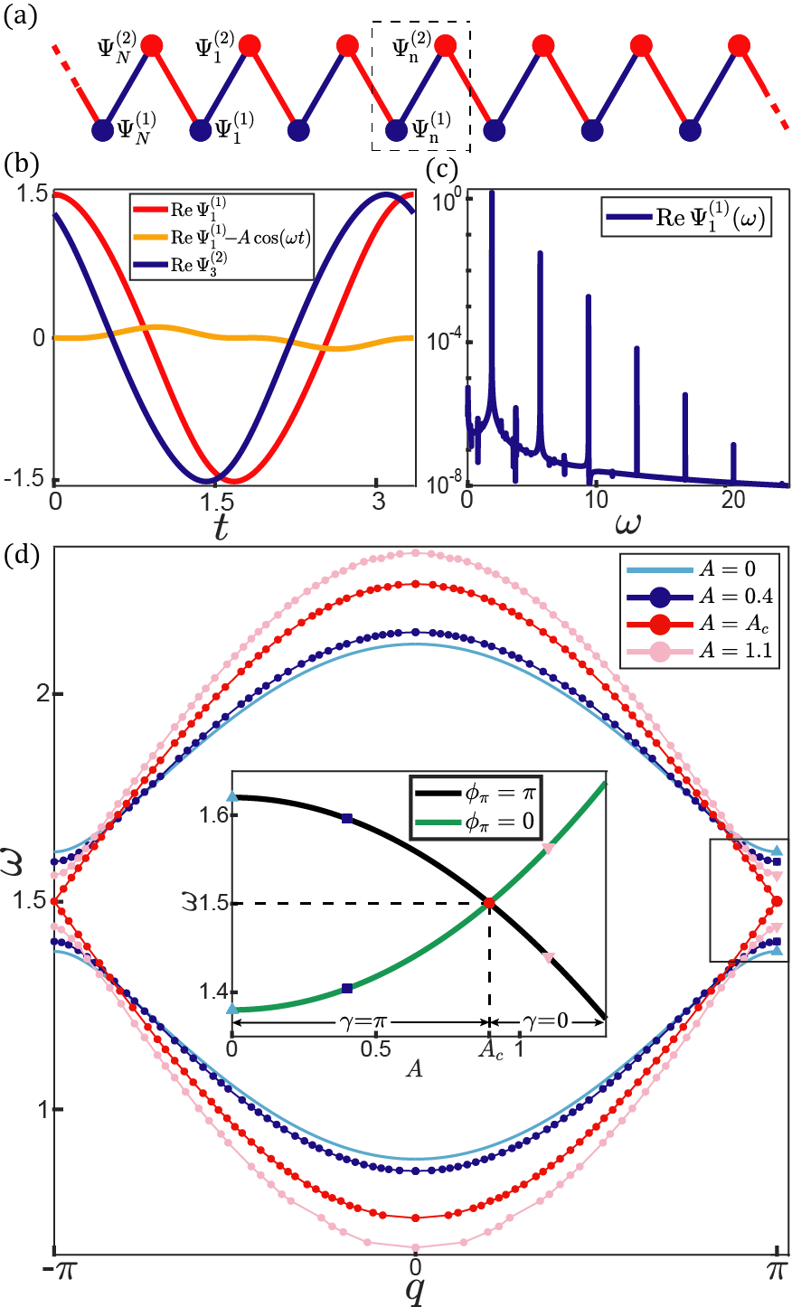
In this paper, we present a systematic study of topological attributes in 1D generalized nonlinear Schrödinger equations beyond Kerr-nonlinearities Hadad et al. (2016). The nonlinear parts of interactions are comparable to the linear ones and perturbation theory breaks down, which we designate the “strongly nonlinear regime”. We limit our considerations within the amplitude range Narisetti et al. (2010); Zaera et al. (2018) that chaos does not occur. Consequently, nonlinear bulk modes Vakakis et al. (2001); Fronk and Leamy (2017) are remarkably distinct from sinusoidal waves (e.g., fig.1(b) and fig.D6(c)). We develop the proper definition of Berry phase in nonlinear bulk modes. By adopting a symmetry-based analytic treatment, we demonstrate the quantization of Berry phase in reflection-symmetric systems, regardless of the availability of linear analysis. The emergence of nonlinear topological edge modes is associated with a quantized Berry phase that protects them from defects. Finally, instead of exponentially localizing on lattice boundaries, topological edge modes exhibit anomalous behaviors that decay to a plateau governed by the stable fixed points of nonlinearities.

II Quantized Berry phase of nonlinear bulk modes

Generalized nonlinear Schrödinger equations are widely studied in classical systems like nonlinear optics Smirnova et al. (2020); Scalora et al. (2005) and electrical circuits Hadad et al. (2018). Their equations of motion are summarized as the general form in Eqs.(1) below. We study nonlinear bulk modes, from which we define Berry phase and demonstrate its quantization in reflection-symmetric models.

The considered model is a nonlinear SSH Su et al. (1979) chain composed of NN classical dimer fields Ψn=(Ψn(1),Ψn(2))\Psi_{n}=(\Psi_{n}^{(1)},\Psi_{n}^{(2)})^{\top} (\top is matrix transpose) coupled by nonlinear interactions, as represented pictorially in Fig.1(a). The chain dynamics is governed by the 1D generalized nonlinear Schrödinger equations,

itΨn(1)=ϵ0Ψn(1)+f1(Ψn(1),Ψn(2))+f2(Ψn(1),Ψn1(2)),\displaystyle\mathrm{i}\partial_{t}\Psi^{(1)}_{n}=\epsilon_{0}\Psi^{(1)}_{n}+f_{1}(\Psi^{(1)}_{n},\Psi_{n}^{(2)})+f_{2}(\Psi^{(1)}_{n},\Psi^{(2)}_{n-1}), (1)
itΨn(2)=ϵ0Ψn(2)+f1(Ψn(2),Ψn(1))+f2(Ψn(2),Ψn+1(1)),\displaystyle\mathrm{i}\partial_{t}\Psi^{(2)}_{n}=\epsilon_{0}\Psi^{(2)}_{n}+f_{1}(\Psi^{(2)}_{n},\Psi^{(1)}_{n})+f_{2}(\Psi^{(2)}_{n},\Psi^{(1)}_{n+1}),

subjected to periodic boundary condition (PBC), where ϵ00\epsilon_{0}\geq 0 is the on-site potential, and fi(x,y)f_{i}(x,y) for i=1i=1 and i=2i=2 stand for intracell and intercell nonlinear couplings, respectively. fi(x,y)f_{i}(x,y) are real-coefficient general polynomials of xx, xx^{*}, yy, and yy^{*} (* represents complex conjugate), which offer time-reversal symmetry Hasan and Kane (2010). Given a nonlinear solution Ψn(t)\Psi_{n}(t), time-reversal symmetry demands a partner solution Ψn(t)\Psi_{n}^{*}(-t), as demonstrated in App. B1. For systems such as those with Bose-Einstein condensates Leggett (2001), |Ψ(r,t)|2|\Psi(\vec{r},t)|^{2} corresponds to a particle number density and third-order nonlinearities are thus limited to |Ψ|2Ψ|\Psi|^{2}\Psi to enforce particle number conservation; in our case the fields do not correspond to particle densities and more general nonlinearities are thus permitted.

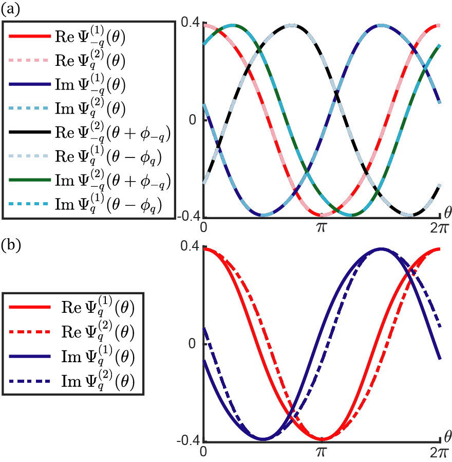
In linear regime, the polynomials are approximated as fi(x,y)ciyf_{i}(x,y)\approx c_{i}y (ci=1,2>0c_{i=1,2}>0) to have “gapped” two-band models when c1c2c_{1}\neq c_{2}. The bulk mode eigenfunctions are sinusoidal in time, and Berry phase is quantized by reflection symmetry. In the “strongly nonlinear regime” where nonlinear interactions become comparable to the linear ones, nonlinear bulk modes are significantly different from sinusoidal waves (e.g. figs.1(b), D6(c)), and the frequencies naturally deviate from their linear counterparts. The nonlinearities become increasingly important as the bulk mode amplitude rises. Hence, the frequency of a nonlinear bulk mode is controlled both by wavenumber and amplitude. We thus define nonlinear band structure Hadad et al. (2018, 2016) ω=ω(q[π,π],A)\omega=\omega(q\in[-\pi,\pi],A) as the frequencies of nonlinear bulk modes for given amplitude AA. We consider the simple case that nonlinear bulk modes are always non-degenerate (i.e., different modes at the same wavenumber have different frequencies) unless they reach the topological transition amplitude when the nonlinear bands merge at the band-touching frequency. Hence, given the amplitude, frequency, and wavenumber, a nonlinear bulk mode is uniquely defined. Extended from gapped linear models, the lattice is a “gapped two-band nonlinear model”. In what follows, we define Berry phase for nonlinear bulk modes of the upper-band by adiabatically evolving the wavenumber across the Brillouin zone.

The considered nonlinear bulk mode is spatial-temporal periodic. It takes the traveling plane-wave ansatz,

Ψq=(Ψq(1)(ωtqn),Ψq(2)(ωtqn+ϕq)),\displaystyle\Psi_{q}=(\Psi_{q}^{(1)}(\omega t-qn),\Psi_{q}^{(2)}(\omega t-qn+\phi_{q}))^{\top}, (2)

where ω\omega and qq are the frequency and wavenumber, respectively. Ψq(j=1,2)(θ)\Psi_{q}^{(j=1,2)}(\theta) are 2π2\pi-periodic wave components, where the phase conditions are chosen by asking ReΨq(j)(θ=0)=A{\rm Re\,}\Psi_{q}^{(j)}(\theta=0)=A, and A=defmax(ReΨq(j))A\overset{\rm def}{=}\max({\rm Re\,}\Psi_{q}^{(j)}) is the amplitude. This is analogous to the phase condition ReΨ(t=0)=max(ReΨ(t)){\rm Re\,}\Psi(t=0)=\max({\rm Re\,}\Psi(t)) adopted in Schrödinger equation in order to have the eigenfunctions Ψ(t)=|Ψ|eiϵt/\Psi(t)=|\Psi|e^{-\mathrm{i}\epsilon t/\hbar}. Following this condition, ϕq\phi_{q} in Eq.(2) characterizes the relative phase between the two wave components. Nonlinear bulk modes are not sinusoidal. They fulfill itΨq=H(Ψq)\mathrm{i}\partial_{t}\Psi_{q}=H(\Psi_{q}), where H(Ψq)H(\Psi_{q}) is the nonlinear function determined by Eqs.(1) and is elaborated in App. A. Given the band index and the amplitude AA of a nonlinear bulk mode, we find that ω\omega, ϕq\phi_{q}, and the waveform are determined by the wavenumber qq.

We adopt the ansatz in Eq.(2) based on a number of reasons. First, typical studies on weakly nonlinear bulk modes Vila et al. (2019); Fronk and Leamy (2017); Pal et al. (2018); Zhou et al. (2020); Narisetti et al. (2010); Zaera et al. (2018); Vakakis et al. (2001) reveal that the dynamics of all high-order harmonics are controlled by the single variable θ=ωtqn\theta=\omega t-qn: Ψq(j)=lψl,q(j)eil(ωtqn)\Psi_{q}^{(j)}=\sum_{l}\psi_{l,q}^{(j)}e^{-\mathrm{i}l(\omega t-qn)}, where ψl,q(j)=(2π)102πeilθΨq(j)𝑑θ\psi_{l,q}^{(j)}=(2\pi)^{-1}\int_{0}^{2\pi}e^{\mathrm{i}l\theta}\Psi_{q}^{(j)}d\theta is the ll-th Fourier component of Ψq(j)\Psi_{q}^{(j)}. Second, numerical experiments such as shooting method (see figs.1(b), D6(a,c), and Refs. Renson et al. (2016); Ha (2001); Peeters et al. (2008)) manifest non-dispersive, plane-wave like bulk modes in the strongly nonlinear regime. Finally, it is demonstrated in App. C3 that the analytic solutions of nonlinear bulk modes at high-symmetry wavenumbers are in perfect agreement with Eq.(2).

We realize the adiabatic evolution of wavenumber q(t)q(t^{\prime}) traversing the Brillouin zone from q(0)=qq(0)=q to q(t)=q+2πq(t)=q+2\pi, while the amplitude AA remains unchanged during this process. According to the nonlinear extension of the adiabatic theorem Xiao et al. (2010); Liu et al. (2003); Pu et al. (2007); Liu and Fu (2010), a system H(Ψq)H(\Psi_{q}) initially in one of the nonlinear modes Ψq\Psi_{q} will stay as an instantaneous nonlinear mode of H(Ψq(t))H(\Psi_{q(t)}) throughout this procedure, provided that the nonlinear mode Ψq\Psi_{q} is stable Pu et al. (2007) within the amplitude scope of this paper. The stability of nonlinear bulk modes is confirmed in App. C via the algorithm of self-oscillation Fronk and Leamy (2017); Vila et al. (2019); Pal et al. (2018). Therefore, the only degree of freedom is the phase of mode. At time tt, the mode is Ψq(t)(0tω(t,q(t))𝑑tγ(t))\Psi_{q(t)}(\int_{0}^{t}\omega(t^{\prime},q(t^{\prime}))dt^{\prime}-\gamma(t)), where γ(t)\gamma(t) defines the phase shift of the nonlinear bulk mode in the adiabatic evolution. The dynamics of γ\gamma is depicted by (dγ/dt)(Ψq/θ)=(dq/dt)(Ψq/q)(d\gamma/dt)(\partial\Psi_{q}/\partial\theta)=(dq/dt)(\partial\Psi_{q}/\partial q). After qq traverses the Brillouin zone, the wave function acquires an extra phase γ\gamma dubbed Berry phase of nonlinear bulk modes,

γ=BZ𝑑ql𝒵(l|ψl,q(2)|2ϕqq+ijψl,q(j)ψl,q(j)q)l𝒵l(j|ψl,q(j)|2),\displaystyle\gamma=\oint_{\rm BZ}dq\frac{\sum_{l\in\mathcal{Z}}\left(l|\psi_{l,q}^{(2)}|^{2}\frac{\partial\phi_{q}}{\partial q}+\mathrm{i}\sum_{j}\psi_{l,q}^{(j)*}\frac{\partial\psi_{l,q}^{(j)}}{\partial q}\right)}{\sum_{l^{\prime}\in\mathcal{Z}}l^{\prime}\left(\sum_{j^{\prime}}|\psi_{l^{\prime},q}^{(j^{\prime})}|^{2}\right)},\quad (3)

where j,j=1,2j,j^{\prime}=1,2 denote the two wave components, and the mathematical derivations are in App. A. In general, γ\gamma is not quantized unless additional symmetry properties are imposed on the model, which we will discuss below. We note that the eigenmodes of linear problems are sinusoidal in time, which reduces Eq.(3) to the conventional form Xiao et al. (2010) γ=BZdqiΨq|q|Ψq\gamma=\oint_{\rm BZ}\mathrm{d}q\,\mathrm{i}\langle\Psi_{q}|\partial_{q}|\Psi_{q}\rangle.

Now we demonstrate that Berry phase defined in Eq.(3) is quantized by reflection symmetry. The model in Eqs.(1) respects reflection symmetry, which means that the nonlinear equations of motion are invariant under reflection transformation,

(Ψn(1),Ψn(2))(Ψn(2),Ψn(1)).\displaystyle(\Psi^{(1)}_{n},\Psi^{(2)}_{n})\to(\Psi^{(2)}_{-n},\Psi^{(1)}_{-n}). (4)

Given a nonlinear bulk mode Ψq\Psi_{q} in Eq.(2), reflection transformation demands a partner solution Ψq=(Ψq(2)(ωt+qn),Ψq(1)(ωt+qnϕq))\Psi_{-q}^{\prime}=(\Psi^{(2)}_{q}(\omega t+qn),\Psi^{(1)}_{q}(\omega t+qn-\phi_{q}))^{\top} that also satisfies the model. On the other hand, a nonlinear bulk mode of wavenumber q-q is by definition denoted as Ψq=(Ψq(1)(ωt+qn),Ψq(2)(ωt+qn+ϕq))\Psi_{-q}=(\Psi_{-q}^{(1)}(\omega t+qn),\Psi_{-q}^{(2)}(\omega t+qn+\phi_{-q}))^{\top}. Since there is no degeneracy of nonlinear bulk modes, Ψq\Psi_{-q}^{\prime} and Ψq\Psi_{-q} have to be identical, which imposes the constraints

ϕq=ϕqmod2π,andΨq(2)=Ψq(1).\displaystyle\phi_{-q}=-\phi_{q}\mod 2\pi,\quad{\rm and}\quad\Psi^{(2)}_{q}=\Psi^{(1)}_{-q}. (5)

Thus, the Fourier components of nonlinear bulk modes satisfy ψl,q(2)=ψl,q(1)\psi_{l,q}^{(2)}=\psi_{l,-q}^{(1)}. This relationship, together with Eqs.(5), is the key to quantizing the Berry phase in Eq.(3) (details in App. B2),

γ=12BZdϕqdq𝑑q=ϕπϕ0=0orπmod2π,\displaystyle\gamma=\frac{1}{2}\oint_{\rm BZ}\frac{d\phi_{q}}{dq}dq=\phi_{\pi}-\phi_{0}=0{\rm\,\,or\,\,}\pi\mod 2\pi, (6)

where ϕq=0,π\phi_{q=0,\pi} are the relative phases of the upper-band nonlinear modes at high-symmetry points. They are determined by comparing the frequencies ω(ϕq=0)\omega(\phi_{q}=0) and ω(ϕq=π)\omega(\phi_{q}=\pi) for q=0q=0 and π\pi. γ=π\gamma=\pi if ω(ϕ0=0)\omega(\phi_{0}=0) and ω(ϕπ=π)\omega(\phi_{\pi}=\pi) belong to the same band, whereas γ=0\gamma=0 if they are in different bands. Interestingly, γ\gamma encounters a topological transition induced by the critical amplitude A=AcA=A_{c} if frequencies merge at ω(ϕπ=0,Ac)=ω(ϕπ=π,Ac)\omega(\phi_{\pi}=0,A_{c})=\omega(\phi_{\pi}=\pi,A_{c}). This transition is exemplified by the minimal model of nonlinear topological lattice in Sec.III. It is worth emphasizing that despite all the discussions of nonlinear Schrödinger equations and the quantization of Berry phase, the model is purely classical in the sense of \hbar being zero.

Refer to caption
Figure 1: The minimal model of nonlinear SSH chain. (a), schematic illustration of the lattice subjected to PBC. Unit cell is enclosed by black dashed box. Red and blue bonds represent intracell and intercell couplings. (b), a nonlinear bulk mode computed by shooting method Renson et al. (2016); Ha (2001); Peeters et al. (2008) with amplitude A=1.5A=1.5 and wavenumber q=4π/5q=4\pi/5. Red and blue curves are the wave functions of n=1n=1 and 33 sites, respectively. Orange curve shows the noticeable difference between nonlinear mode and sinusoidal function. (c), frequency profile of nonlinear bulk mode in (b). (d), nonlinear band structures ω=ω(q,A)\omega=\omega(q,A) plotted for bulk mode amplitudes from A=0A=0 to 1.11.1. The red curves touch for the topological transition amplitude Ac=0.8944A_{c}=0.8944 at ω=ϵ0=1.5\omega=\epsilon_{0}=1.5. The inset elaborates the gap-closing transition amplitude AcA_{c} at which band inversion occurs.

Having established quantized Berry phase, we now search additional properties for vanishing on-site potential, ϵ0=0\epsilon_{0}=0. The model’s linear limit respects charge-conjugation symmetry Ryu et al. (2010); Kane and Lubensky (2014), which demands that the states appear in ±ω\pm\omega pairs, and the topological mode have zero-energy. To have ±ω\pm\omega pairs of modes in the nonlinear problem, we require the parity of interactions to satisfy fi(x,y)=fi(x,y)=fi(x,y)f_{i}(-x,y)=-f_{i}(x,-y)=f_{i}(x,y). Consequently, the system is invariant under the transformation (Ψn(1)(ωt),Ψn(2)(ωt))(Ψn(1)(ωt),Ψn(2)(ωt))(\Psi^{(1)}_{n}(\omega t),\Psi^{(2)}_{n}(\omega t))\to(-\Psi^{(1)}_{n}(-\omega t),\Psi^{(2)}_{n}(-\omega t)). Given a nonlinear mode Ψω\Psi_{\omega} defined in Eq.(2), this transformation demands a partner solution Ψω=(Ψq(1)(ωtqn),Ψq(2)(ωtqn+ϕq))\Psi_{-\omega}=(-\Psi^{(1)}_{q}(-\omega t-qn),\Psi^{(2)}_{q}(-\omega t-qn+\phi_{q}))^{\top}. Therefore, nonlinear modes always appear in ±ω\pm\omega pairs. Similar to charge-conjugation symmetric models in linear systems Ryu et al. (2010), the frequencies of nonlinear topological modes are zero, which is illustrated in the following minimal model.

III Topological transition and bulk-boundary correspondence in the minimal model

We now clarify the nonlinear extension of bulk-boundary correspondence Chaunsali and Theocharis (2019); Shang et al. (2018) by demonstrating topological edge modes in the minimal model that respects time-reversal symmetry, where the couplings are specified as

fi(x,y)=ciy+di[(Rey)3+i(Imy)3],\displaystyle f_{i}(x,y)=c_{i}y+d_{i}[({\rm Re\,}y)^{3}+\mathrm{i}({\rm Im\,}y)^{3}], (7)

with ci,di>0c_{i},d_{i}>0 for i=1,2i=1,2. This interaction offers numerically stable nonlinear bulk and topological edge modes and can be realized in passive photonic and active electrical circuit metamaterials (Sec.IV and App. E). We are interested in attributes unique to nonlinear systems, in particular the topological phase transition induced by bulk mode amplitudes. Thus, the parameters yield c1<c2c_{1}<c_{2} and d1>d2d_{1}>d_{2} (c1>c2c_{1}>c_{2} and d1<d2d_{1}<d_{2}) to induce topological-to-non-topological phase transition (non-topological-to-topological transition) as amplitudes increase. We abbreviate them as “T-to-N” and “N-to-T” transitions, and they are converted to one another by simply flipping intracell and intercell couplings. In the remainder of this paper, a semi-infinite lattice subjected to open boundary condition (OBC) is always considered whenever we refer to topological edge modes.
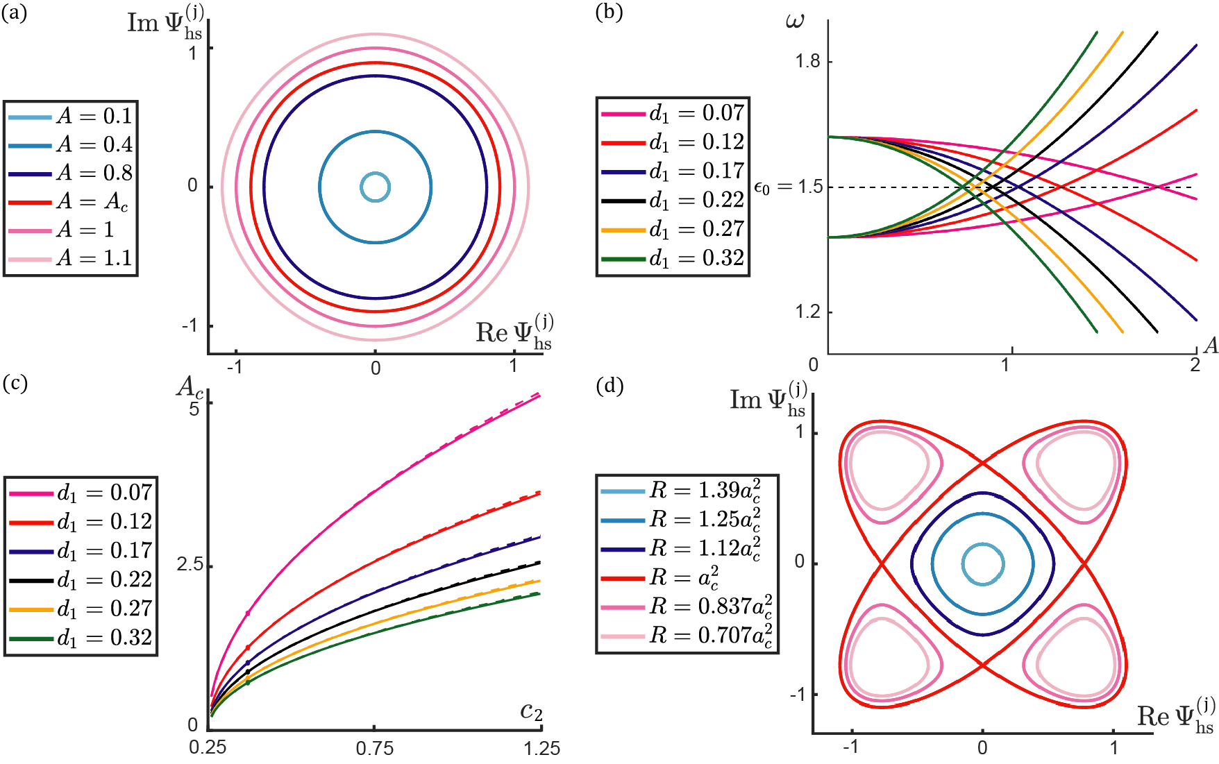
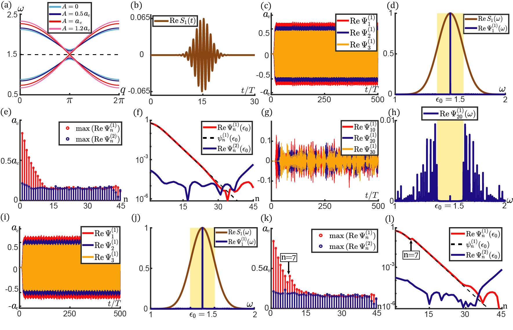
We first study the case c1<c2c_{1}<c_{2} and d1>d2d_{1}>d_{2}, in which a T-to-N transition occurs. Fig.1(d) numerically illustrates nonlinear band structures and topological transition by considering ϵ0=1.5\epsilon_{0}=1.5, c1=0.25c_{1}=0.25, c2=0.37c_{2}=0.37, d1=0.22d_{1}=0.22, and d2=0.02d_{2}=0.02. Given that Berry phase γ(A=0)=π\gamma(A=0)=\pi, the lattice is topologically nontrivial in the linear limit. As amplitudes rise, the topological invariant γ(A<Ac)=π\gamma(A<A_{c})=\pi cannot change until it becomes ill-defined when the nonlinear bandgap closes at the transition amplitude AcA_{c}. The bandgap reopens above AcA_{c}, allowing the well-defined Berry phase to take the trivial value γ(A>Ac)=0\gamma(A>A_{c})=0, as depicted in the inset of Fig.1(d). AcA_{c} is numerically computed by solving the bandgap-closing equation ω(ϕπ=0,Ac)=ω(ϕπ=π,Ac)\omega(\phi_{\pi}=0,A_{c})=\omega(\phi_{\pi}=\pi,A_{c}). We propose a convenient approximation Detroux et al. (2014) f(Ψn(j),Ψn(j))(ci+34diA2)Ψn(j)f(\Psi_{n^{\prime}}^{(j^{\prime})},\Psi_{n}^{(j)})\approx(c_{i}+\frac{3}{4}d_{i}A^{2})\Psi_{n}^{(j)} to estimate the transition amplitude Ac4(c2c1)/3(d2d1)A_{c}\approx\sqrt{-4(c_{2}-c_{1})/3(d_{2}-d_{1})}. The good agreement between this approximation and the numerical solutions is shown in App. C. We highlight that Ac2max(d1,d2)/max(c1,c2)0.5A_{c}^{2}\max(d_{1},d_{2})/\max(c_{1},c_{2})\approx 0.5, which demonstrates the comparable nonlinear and linear interactions in the strongly nonlinear regime.

Refer to caption
Figure 2: Nonlinear edge excitations of the model subjected to T-to-N transition, where the parameters fulfill c1<c2c_{1}<c_{2} and d1>d2d_{1}>d_{2}. (a-d) and (e-h) show lattice boundary responses in small-amplitude topological regime and large-amplitude non-topological regime, respectively. The magnitudes of Gaussian tone bursts are S=7×10²S=7\times 10^{-2} in (a) and S=56×102S=56\times 10^{-2} in (e), respectively. (b) and (f), spatial-temporal profiles of |ReΨn(1)(t)||{\rm Re\,}\Psi_{n}^{(1)}(t)| for all 4545 sites, where |ReΨn(1)(t)||{\rm Re\,}\Psi_{n}^{(1)}(t)| denote the strength of the lattice excitations. (c) and (g), spatial profiles of the frequency spectra of the responding modes, where the time domain of performing Fourier analysis is from 250T250T to 500T500T. White dashed lines mark the top and bottom of the linear bandgap. In (g), modes in the bandgap are triggered by energy absorption Fronk and Leamy (2017) from nonlinear bulk modes. (d) and (h), red and blue curves for the spatial profiles of the ω=ϵ0\omega=\epsilon_{0} wave component of the excitations. The analytic prediction of the topological mode ψn(1)(ϵ0)\psi_{n}^{(1)}(\epsilon_{0}) is depicted by the black dashed curve in (d).

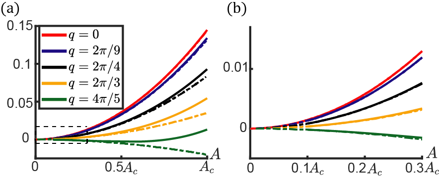
Bulk-boundary correspondence has been extended to weakly nonlinear Newtonian Chaunsali and Theocharis (2019) and Schrödinger Shang et al. (2018) systems by showing topological boundary modes guaranteed by topologically non-trivial Berry phase. In the strongly nonlinear problem, we utilize analytic approximation and numerical experiment, to doubly confirm this correspondence by identifying nonlinear topological edge modes. In the former, the lattice is composed of N=45N=45 unit cells with OBCs on both ends to mimic semi-infinite lattice, and the parameters are carried over from Fig.1. The topological mode and frequency are denoted as Ψn=(Ψn(1),Ψn(2))\Psi_{n}=(\Psi_{n}^{(1)},\Psi_{n}^{(2)})^{\top} and ωT\omega_{\rm T}, respectively. Analogous to linear SSH chain Su et al. (1979), the analytic scheme is to approximate Ψn(1)Ψn(2)\Psi_{n}^{(1)}\gg\Psi_{n}^{(2)}, which is numerically verified in Fig.2(d). We make one further approximation to truncate the equations of motion to fundamental harmonics. Therefore, the nonlinear topological edge mode is approximated as Ψn(ψ1,n(1),0)eiϵ0t\Psi_{n}\approx(\psi_{1,n}^{(1)},0)^{\top}e^{-\mathrm{i}\epsilon_{0}t}, where ψ1,n(1)\psi_{1,n}^{(1)} are the fundamental harmonic components. By doing so, we find ωT=ϵ0\omega_{\rm T}=\epsilon_{0}, and

(c1+34d1|ψ1,n(1)|2)|ψ1,n(1)|=(c2+34d2|ψ1,n+1(1)|2)|ψ1,n+1(1)|.\displaystyle\left(c_{1}+\frac{3}{4}d_{1}|\psi_{1,n}^{(1)}|^{2}\right)|\psi_{1,n}^{(1)}|=\left(c_{2}+\frac{3}{4}d_{2}|\psi_{1,n+1}^{(1)}|^{2}\right)|\psi_{1,n+1}^{(1)}|.

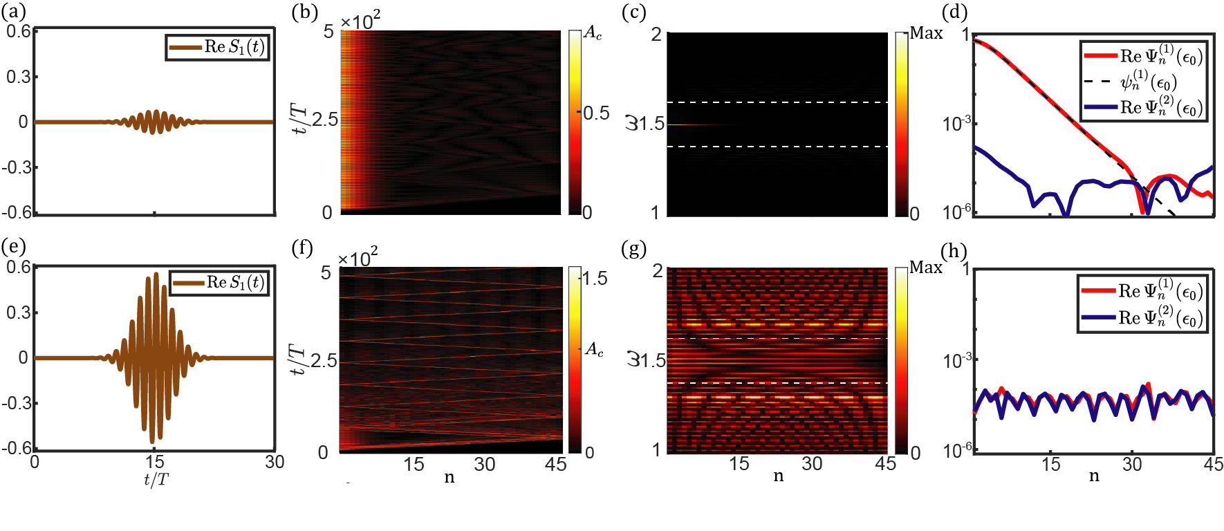
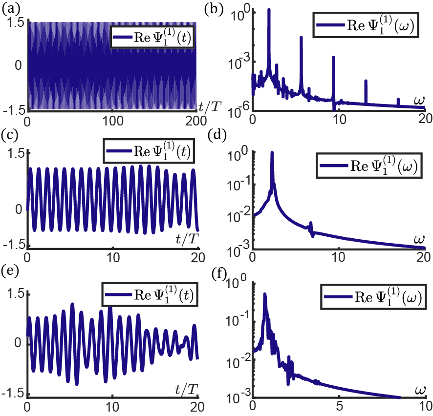
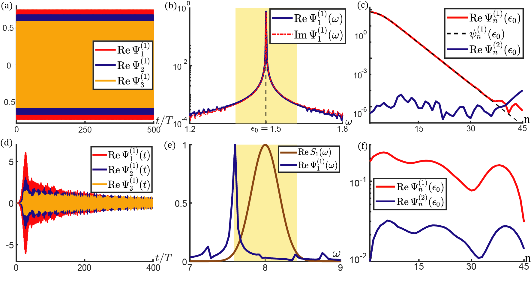
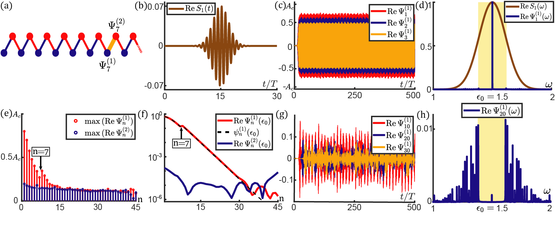
From Eq.(III), the semi-infinite lattice hosts topological evanescent modes when |Ψ1(1)|<4(c2c1)/3(d2d1)Ac|\Psi_{1}^{(1)}|<\sqrt{-4(c_{2}-c_{1})/3(d_{2}-d_{1})}\approx A_{c}, whereas no such mode exists for |Ψ1(1)|>4(c2c1)/3(d2d1)Ac|\Psi_{1}^{(1)}|>\sqrt{-4(c_{2}-c_{1})/3(d_{2}-d_{1})}\approx A_{c}. In App. D, the frequency and analytic expression are applied in weakly nonlinear regime, and they are perfectly in line with method of multiple-scale Fronk and Leamy (2017); Narisetti et al. (2010); Zaera et al. (2018); Snee and Ma (2019). The numerical scenario is accomplished by applying a Gaussian profile signal Sn=δn1Seiωextt(tt0)2/τ2(1,0)S_{n}=\delta_{n1}Se^{-\mathrm{i}\omega_{\rm ext}t-(t-t_{0})^{2}/\tau^{2}}(1,0)^{\top} on the first site, where the carrier frequency ωext=ϵ0=1.5\omega_{\rm ext}=\epsilon_{0}=1.5, T=2π/ωextT=2\pi/\omega_{\rm ext}, τ=3T\tau=3T controls Gaussian spread, and t0=15Tt_{0}=15T denotes trigger time. Figs.2(b) and (f) together verify bulk-boundary correspondence Chaunsali and Theocharis (2019); Shang et al. (2018) by identifying the presence and absence of topological boundary excitations below and above the critical amplitude AcA_{c}, respectively. In fig.2(d), the flattened part near the lattice boundary is the manifestation of nonlinearities.

One may find it unusual that the frequencies of topological modes ωT=ϵ0\omega_{\rm T}=\epsilon_{0} are independent of amplitudes, although this result is in agreement with Ref. Hadad et al. (2018, 2016); Chaunsali and Theocharis (2019) in weakly nonlinear regime. Here we propose an explanation for this intriguing result. Because the evanescent mode fades to zero in the bulk, the “tail” of this mode eventually enters into small-amplitude regime where nonlinearities are negligible and linear analysis becomes effective. Linear topological theory Su et al. (1979) demands the tail of the mode to be ωT=ϵ0\omega_{\rm T}=\epsilon_{0}, which in turn requires the frequency of the nonlinear topological mode to be independent of the amplitude.

Topological protection is featured in multiple aspects. As visualized in Fig.1(d), the frequencies of topological modes stay in the bandgap and are distinct from nonlinear bulk modes. The appearance and absence of these modes are captured by the topological invariant that cannot change continuously upon the variation of system parameters. Lastly, topological modes are insensitive to defects, which is numerically verified in App. D.
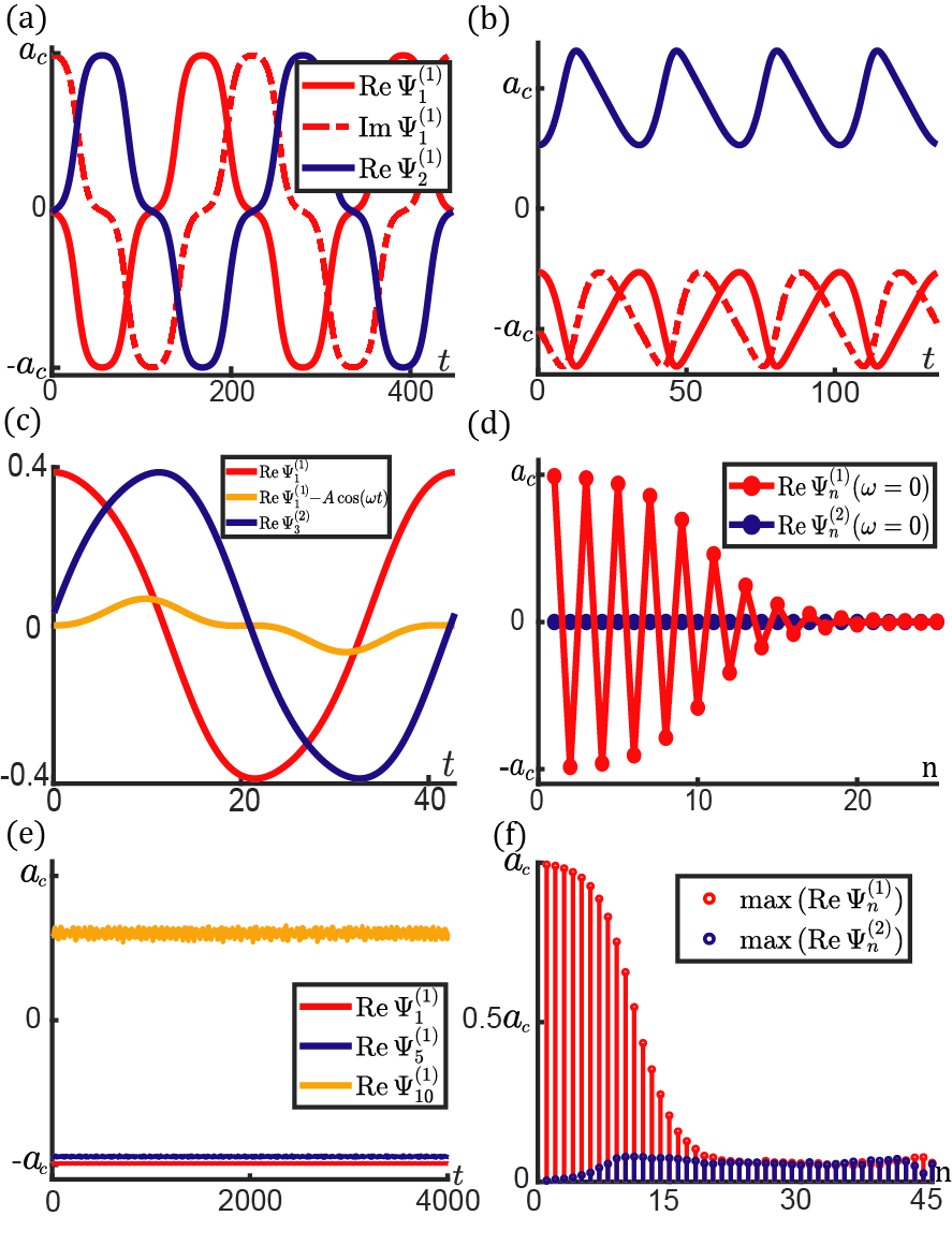
When ϵ0=0\epsilon_{0}=0, the model manifests nonlinear bulk modes in ±ω\pm\omega pairs. Topologically protected nonlinear boundary modes do not oscillate in time, in contrast to the ϵ00\epsilon_{0}\neq 0 systems. Thus, we obtain exact solutions of nonlinear topological modes via the recursion relation, f1(Ψn(1),Ψn(2))+f2(Ψn(1),Ψn1(2))=f1(Ψn(2),Ψn(1))+f2(Ψn(2),Ψn+1(1))=0f_{1}(\Psi_{n}^{(1)},\Psi^{(2)}_{n})+f_{2}(\Psi_{n}^{(1)},\Psi^{(2)}_{n-1})=f_{1}(\Psi_{n}^{(2)},\Psi^{(1)}_{n})+f_{2}(\Psi_{n}^{(2)},\Psi^{(1)}_{n+1})=0. This is the nonlinear analog of charge-conjugation symmetric systems.
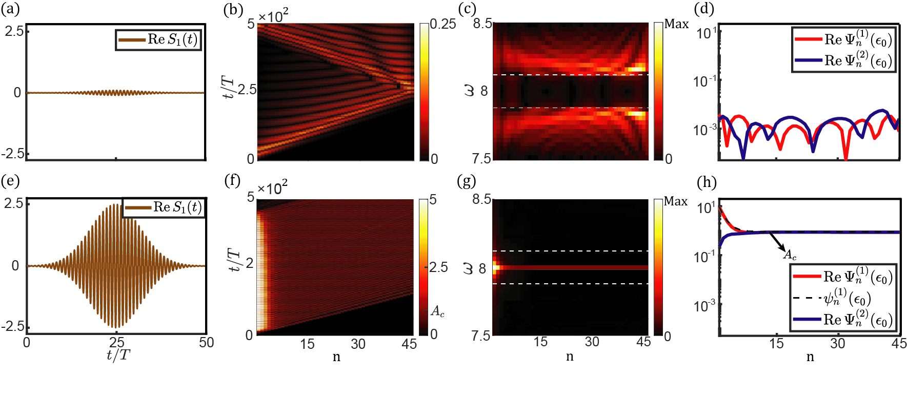
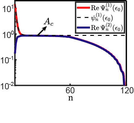
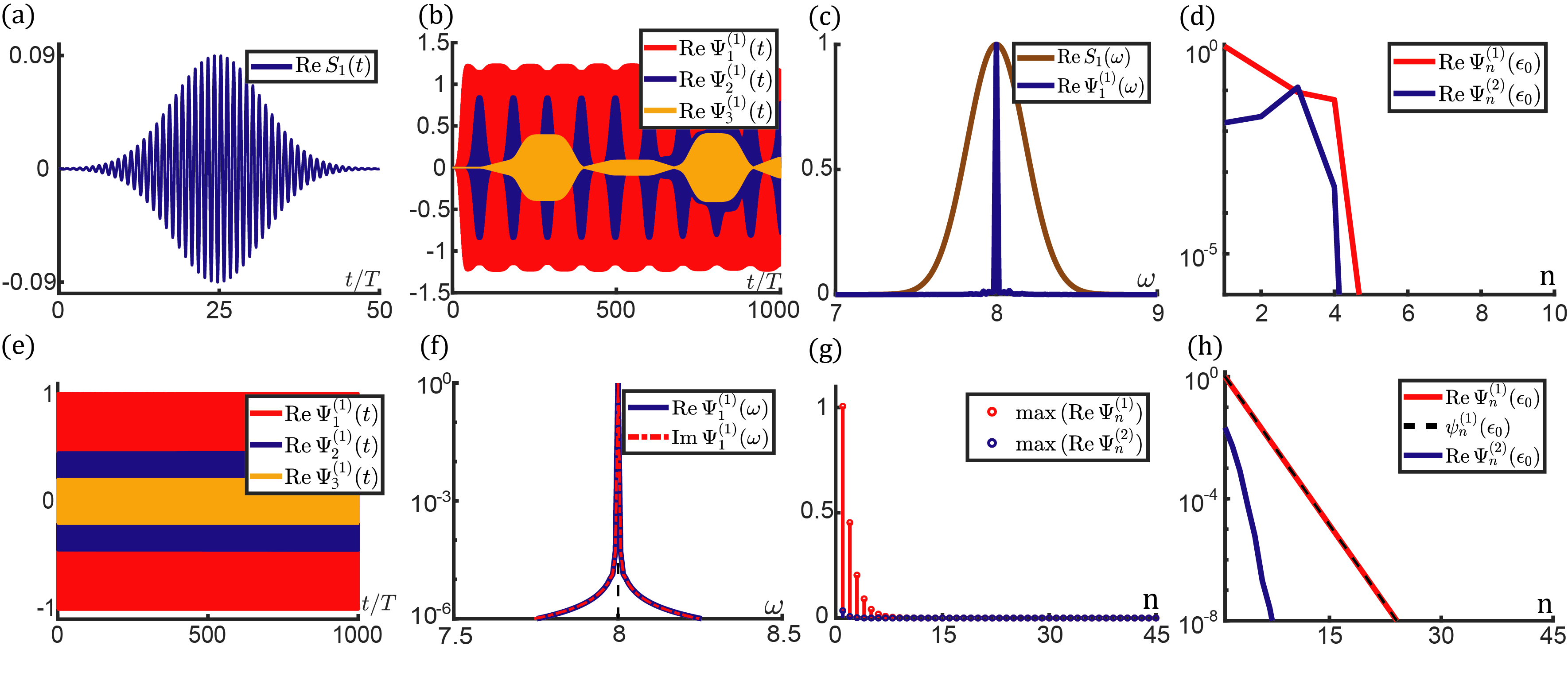
Refer to caption
Figure 3: Nonlinear boundary responses of the lattice subjected to N-to-T transition, where the parameters yield c1>c2c_{1}>c_{2} and d1<d2d_{1}<d_{2}. (a-d) and (e-h) exhibit lattice boundary excitations in the small-amplitude non-topological regime and the large-amplitude topological regime, respectively. The magnitudes of Gaussian signals are S=0.1S=0.1 in (a) and S=2.5S=2.5 in (e), respectively. (b) and (f), Spatial-temporal profiles of |ReΨn(1)(t)||{\rm Re\,}\Psi_{n}^{(1)}(t)| for 4545 sites. (c) and (g), frequency spectra of the lattice excitations for 4545 sites. Fourier analysis is executed from 250T250T to 500T500T. White dashed lines encircle the linear bandgap. (d) and (h), red and blue curves for the spatial distributions of the ω=ϵ0\omega=\epsilon_{0} mode component of the lattice excitations. The analytic result of the anomalous topological modes ψn(1)(ϵ0)\psi_{n}^{(1)}(\epsilon_{0}) is captured by the black dashed curve in (h).

In the second case of c1>c2c_{1}>c_{2} and d1<d2d_{1}<d_{2}, N-to-T (non-topological-to-topological) transition occurs as amplitudes rise. We exemplify boundary excitations in Fig.3 by letting ϵ0=8\epsilon_{0}=8, c1=0.37c_{1}=0.37, c2=0.25c_{2}=0.25, d1=0.02d_{1}=0.02, and d2=0.22d_{2}=0.22. A Gaussian signal is applied on the first site of the lattice, where the carrier frequency ωext=ϵ0=8\omega_{\rm ext}=\epsilon_{0}=8, T=2π/ωextT=2\pi/\omega_{\rm ext}, Gaussian spread τ=10T\tau=10T, and trigger time t0=25Tt_{0}=25T. In the small-amplitude regime, we consider a chain of N=45N=45 unit cells. As shown in Fig.3(b), the lattice is free of topological modes for |Ψ1(1)|<Ac=0.8944|\Psi_{1}^{(1)}|<A_{c}=0.8944. In the large-amplitude regime, the lattice is constructed from N=120N=120 unit cells. Anomalous topological edge modes emerge when |Ψ1(1)|>Ac|\Psi_{1}^{(1)}|>A_{c} (see figs.3(f,h)). In contrast to conventional topological modes that shrink to zero over space, Ψn(1)\Psi_{n}^{(1)} decay to the plateau AcA_{c} governed by the stable fixed point of Eq.(III), whereas Ψn(2)\Psi_{n}^{(2)} increase to AcA_{c} by absorbing energy Fronk and Leamy (2017) from Ψn(1)\Psi_{n}^{(1)}. Theoretical analysis predicts that the plateau should extend to infinity, but the plateau is limited to reach site 6060 by the finite lifetime of topological modes due to the energy conversion to bulk modes, as elaborated in Fig.D2. Despite the huge nonlinearities (|Ψ1(1)|/Ac10|\Psi_{1}^{(1)}|/A_{c}\sim 10, and |Ψ1(1)|2max(d1,d2)/max(c1,c2)10|\Psi_{1}^{(1)}|^{2}\max(d_{1},d_{2})/\max(c_{1},c_{2})\sim 10), this mode is stable within the finite lifetime of more than 400 periods. This model serves as the combined prototype of long-lifetime, high-energy storage, long-distance transmission of topological modes, and efficient frequency converter from Gaussian inputs to monochromatic signals.

Although T-to-N and N-to-T transitions are converted to one another by choosing the unit cell, topological modes behave qualitatively different (Fig.2(d) and 3(h)) due to the distinction in the fixed points of Eq.(III). The modes converge to the stable fixed point 0 in T-to-N transition (AcA_{c} in N-to-T transition), but this fixed point becomes unstable in N-to-T transition (T-to-N transition).

IV Proposals for experimental implementations

Upon establishing nonlinear topological band theory, it is natural to ask if any realistic physical systems enjoy these unconventional properties. Classical passive and active structures are proposed here to realize the minimal model of Eq.(7), as detailed in App. E.

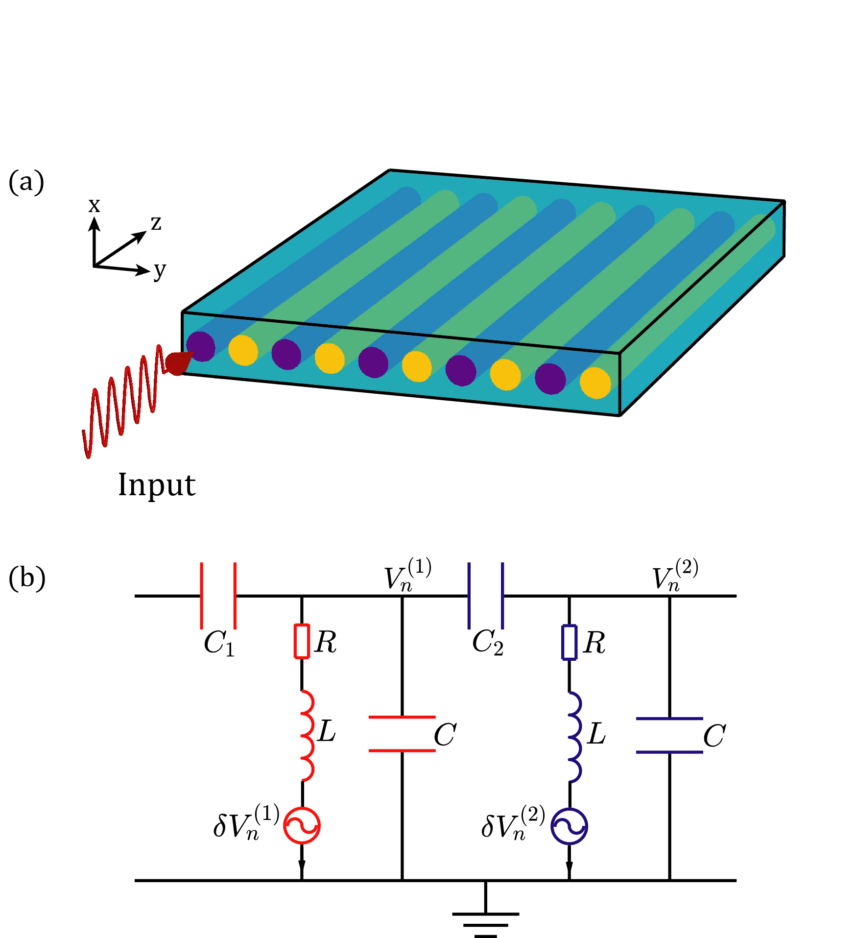
Topological photonics D’Aguanno et al. (2008); Christodoulides and Joseph (1988), passive system: Our theoretical prototype is readily testified in 1D array of optic lattice. Each unit cell is composed of two waveguides to guide electro-magnetic modes along the axial direction, and the permittivity and permeability are nonlinearly modulated by the fields. Hence, the adjacent electro-magnetic fields are coupled nonlinearly. It can be shown that the propagation of electro-magnetic fields along the axial zz-direction is depicted by 4-field extension of generalized nonlinear Schrödinger equations, where the zz-coordinate takes place of the time-like differential variable D’Aguanno et al. (2008); Christodoulides and Joseph (1988). Consequently, this photonic system realizes the minimal model of Eq.(7).

Topoelectrical circuit Hadad et al. (2018), active system: The second promising direction is to construct a ladder of cascaded diatomic unit cells composed of two LCR resonators and two capacitors Cj=1,2CC_{j=1,2}\ll C. The inductances are connected to external power sources which are nonlinear functions of Vn(j=1,2)V_{n}^{(j=1,2)}. The motion equation of the unit cell voltages Vn(j=1,2)V_{n}^{(j=1,2)} are captured by Eqs.(1) and Eq.(7), and nonlinear topological attributes can be studied here.

Refer to caption
Figure 4: Experimental proposals for passive and active nonlinear topological metamaterials. (a) 1D array of nonlinear optic lattice. The nearest neighbor electro-magnetic fields are coupled nonlinearly. (b) The unit cell of nonlinear active topoelectrical circuit, where the inductances are connected by external alternating power sources nonlinearly controlled by voltage fields Vn(j=1,2)V_{n}^{(j=1,2)}.

V Conclusions

In this paper, we extend topological band theory to strongly nonlinear Schrödinger equations beyond Kerr-type nonlinearities. The proper definition of Berry phase is carried out for nonlinear bulk modes, and its quantization is demonstrated in reflection-symmetric models. The topological invariant experiences transitions induced by mode amplitudes. These results can be extended to higher dimensional systems with arbitrarily complex unit cells, but we leave the full proof for the future.

The advent (disappearance) of topological modes is associated with a change in the Berry phase to its topological (non-topological) value. As amplitudes increase, T-to-N (topological-to-non-topological) and N-to-T (non-topological-to-topological) transitions take place for different choices of unit cells. Anomalous topological modes decrease away from lattice boundaries to a plateau controlled by the stable fixed point of nonlinearities.

A rich variety of problems can be studied following this paper, such as the nonlinear extension of topological chiral edge modes in 2D systems Haldane (1988), and higher-order topological states Benalcazar et al. (2017). Experimental characterizations of photonic, acoustic, and electrical metamaterials with built-in nonlinearities can also be studied in future.

Acknowledgements.
D. Z. would like to thank insightful discussions with Xueda Wen, Junyi Zhang, Feng Li, and Biao Wu. This work is supported by the National Key R&\&D Program of China (Grant No. 2020YFA0308800), the NSF of China (Grants Nos. 11734003, 12061131002), and the Strategic Priority Research Program of Chinese Academy of Sciences (Grant No. XDB30000000).

Appendix A Berry phase of nonlinear bulk modes

In this section, we derive Berry phase of nonlinear bulk modes by adiabatically evolving the wave function as the wavenumber qq slowly traverses the Brillouin zone. We consider the nonlinear problem described by a classical two-field generalized nonlinear Schrödinger equations presented in the main text,

itΨn(1)=ϵ0Ψn(1)+f1(Ψn(1),Ψn(2))+f2(Ψn(1),Ψn1(2)),\displaystyle\mathrm{i}\partial_{t}\Psi^{(1)}_{n}=\epsilon_{0}\Psi^{(1)}_{n}+f_{1}(\Psi^{(1)}_{n},\Psi_{n}^{(2)})+f_{2}(\Psi^{(1)}_{n},\Psi^{(2)}_{n-1}),
itΨn(2)=ϵ0Ψn(2)+f1(Ψn(2),Ψn(1))+f2(Ψn(2),Ψn+1(1)),\displaystyle\mathrm{i}\partial_{t}\Psi^{(2)}_{n}=\epsilon_{0}\Psi^{(2)}_{n}+f_{1}(\Psi^{(2)}_{n},\Psi^{(1)}_{n})+f_{2}(\Psi^{(2)}_{n},\Psi^{(1)}_{n+1}),\qquad (9)

where fi(x,y)f_{i}(x,y) for i=1,2i=1,2 are real-coefficient general polynomials of xx, xx^{*}, yy, and yy^{*}. Berry phase is derived from this general model.

In the linear limit, the interactions are approximated as fi(x,y)ciyf_{i}(x,y)\approx c_{i}y (ci=1,2>0c_{i=1,2}>0). The model is a 2×22\times 2 matrix problem in which the bands are gapped. As the amplitude rises, nonlinearities become increasingly significant and the linear bulk modes evolve into nonlinear bulk modes. In this section, we study the simple case that the nonlinear bulk modes are non-degenerate and are stable. In other words, a nonlinear bulk mode is unique, provided that the amplitude AA, the frequency ω\omega, and the wavenumber qq are given. In addition to these properties, we consider the simple case that the nonlinear bandgap Hadad et al. (2018, 2016) never closes. As such, this system is a nonlinear extension of the linear two-band model.

We begin by defining the nonlinear periodic bulk mode of the system as follows,

Ψn(t)=Ψq(ωtqn)=(Ψq(1)(ωtqn)Ψq(2)(ωtqn+ϕq)),\displaystyle\Psi_{n}(t)=\Psi_{q}(\omega t-qn)=\left(\begin{array}[]{c}\Psi_{q}^{(1)}(\omega t-qn)\\ \Psi_{q}^{(2)}(\omega t-qn+\phi_{q})\end{array}\right),\qquad (12)

where qq is the wavenumber and ω\omega is the frequency that belongs to the upper band of the nonlinear band structure. As such, the wave functions depend on the single variable θ=ωtqn\theta=\omega t-qn. We adopt this functional form based on a number of reasons. First, typical studies of weakly nonlinear bulk modes Vila et al. (2019); Fronk and Leamy (2017); Pal et al. (2018); Zhou et al. (2020); Narisetti et al. (2010); Zaera et al. (2018); Vakakis et al. (2001) via the method of multiple-scale reveal that all Fourier components are captured by the single θ\theta variable, Ψn=lψl,neilθ\Psi_{n}=\sum_{l}\psi_{l,n}e^{\mathrm{i}l\theta}. Second, numerical experiments such as shooting method (see figs.1(b), D6(a,c), and Refs. Renson et al. (2016); Ha (2001); Peeters et al. (2008)) manifests non-dispersive bulk modes in strongly nonlinear regime, which appear to be plane-wave like modes. Finally, analytic solutions for special wavenumbers q=0,πq=0,\pi demonstrate that strongly nonlinear bulk modes are in line with Eq.(12). It is at this point that we adopt Eq.(12) as the general form of nonlinear bulk modes.

In general, the waveforms of Ψq(j)(θ)\Psi_{q}^{(j)}(\theta) for j=1,2j=1,2 are not sinusoidal in θ\theta. We note that because the wave function component Ψq(j)(θ)\Psi_{q}^{(j)}(\theta) is 2π2\pi-periodic, it is defined up to an arbitrary phase condition. In this paper, the phase condition is chosen by asking that when θ=0\theta=0, the real part of wave component ReΨq(j)(θ){\rm Re\,}\Psi_{q}^{(j)}(\theta) reaches its amplitude/maximum,

ReΨq(j)(θ=0)=max(ReΨq(j)(θ))=defA,j=1,2.\displaystyle{\rm Re\,}\Psi_{q}^{(j)}(\theta=0)=\max({\rm Re\,}\Psi_{q}^{(j)}(\theta))\overset{\rm def}{=}A,\quad j=1,2.\qquad (13)

Note that the phase condition in Eq.(13) is similar to that in exponential functions, where Reeiθ=0=max(Reeiθ){\rm Re\,}e^{\mathrm{i}\theta=0}=\max({\rm Re\,}e^{\mathrm{i}\theta}). Following this convention, ϕq\phi_{q} in Eq.(12) characterizes the relative phase between Ψq(1)\Psi_{q}^{(1)} and Ψq(2)\Psi_{q}^{(2)}. The nonlinear mode has to fulfill the differential equation parametrized by wavenumber qq,

itΨq(θ)=H(Ψq),\displaystyle\mathrm{i}\partial_{t}\Psi_{q}(\theta)=H(\Psi_{q}), (14)

where θ=ωt\theta=\omega t, and the nonlinear function H(Ψq)H(\Psi_{q}) is given by

H(Ψq)\displaystyle H(\Psi_{q}) =\displaystyle= (ϵ0Ψq(1)(θ)ϵ0Ψq(2)(θ+ϕq))\displaystyle\left(\begin{array}[]{c}\epsilon_{0}\Psi_{q}^{(1)}(\theta)\\ \epsilon_{0}\Psi_{q}^{(2)}(\theta+\phi_{q})\\ \end{array}\right) (23)
+(f1(Ψq(1)(θ),Ψq(2)(θ+ϕq))f1(Ψq(2)(θ+ϕq),Ψq(1)(θ)))\displaystyle+\left(\begin{array}[]{c}f_{1}(\Psi_{q}^{(1)}(\theta),\Psi_{q}^{(2)}(\theta+\phi_{q}))\\ f_{1}(\Psi_{q}^{(2)}(\theta+\phi_{q}),\Psi_{q}^{(1)}(\theta))\\ \end{array}\right)
+(f2(Ψq(1)(θ),Ψq(2)(θ+q+ϕq))f2(Ψq(2)(θ+ϕq),Ψq(1)(θq))).\displaystyle+\left(\begin{array}[]{c}f_{2}(\Psi_{q}^{(1)}(\theta),\Psi_{q}^{(2)}(\theta+q+\phi_{q}))\\ f_{2}(\Psi_{q}^{(2)}(\theta+\phi_{q}),\Psi_{q}^{(1)}(\theta-q))\\ \end{array}\right).

In what follows, we study the nonlinear bulk mode with the fixed amplitude AA. Therefore, the mode frequency ω\omega, the relative phase ϕq\phi_{q}, and the waveform are controlled by the wavenumber qq.

Next, we adiabatically evolve the wavenumber q(t)q(t) traversing the Brillouin zone from q(0)=qq(0)=q to q(t)=q+2πq(t)=q+2\pi. According to the nonlinear extension of adiabatic theorem Xiao et al. (2010); Liu et al. (2003); Pu et al. (2007); Liu and Fu (2010), a system initially in one of its nonlinear mode Ψq\Psi_{q} of the upper band will stay as an instantaneous upper-band nonlinear mode of H(Ψq(t))H(\Psi_{q(t)}) throughout the process. This theorem is valid when the control parameter qq varies sufficiently slowly compared to the frequencies Liu et al. (2003), and the nonlinear bulk modes are stable Pu et al. (2007) within the amplitude scope of this paper. In App. C, we exploit the self-oscillation method Fronk and Leamy (2017) to confirm the stability of these nonlinear modes. Hence the only degree of freedom is the phase of the mode. At time tt, the mode is

Ψq(t)(0tω(t,q(t))𝑑tγ(t)).\displaystyle\Psi_{q(t)}\left(\int_{0}^{t}\omega(t^{\prime},q(t^{\prime}))dt^{\prime}-\gamma(t)\right). (24)

We are interested in the extra phase term γ\gamma, which will be carried out as follows. Substituting Eq.(24) into Eq.(14), we have

dγdtΨqθ=dqdtΨqq,\displaystyle\frac{d\gamma}{dt}\frac{\partial\Psi_{q}}{\partial\theta}=\frac{dq}{dt}\frac{\partial\Psi_{q}}{\partial q}, (25)

where θ=ωt\theta=\omega t stands for the phase of the wave function Ψq\Psi_{q}. We bare in mind that the nonlinear bulk mode is 2π2\pi-periodic in its phase, which grants Fourier transformation. We expand Ψq(j)(θ)\Psi_{q}^{(j)}(\theta), the component of periodic wave function, in terms of its Fourier series:

Ψq(j)(θ)=l𝒵ψl,q(j)eilθj=1,2,\displaystyle\Psi_{q}^{(j)}(\theta)=\sum_{l\in\mathcal{Z}}\psi_{l,q}^{(j)}e^{-\mathrm{i}l\theta}\qquad j=1,2, (26)

where ψl,q(j)\psi_{l,q}^{(j)} is the ll-th Fourier component of Ψq(j)\Psi_{q}^{(j)} (ll is integer). Inserting Eq.(26) into Eq.(25), we have

dγdtlileilθ(ψl,q(1)ψl,q(2)eilϕq)=\displaystyle\frac{d\gamma}{dt}\sum_{l}\mathrm{i}le^{-\mathrm{i}l\theta}\left(\begin{array}[]{c}\psi_{l,q}^{(1)}\\ \psi_{l,q}^{(2)}e^{-\mathrm{i}l\phi_{q}}\\ \end{array}\right)= (29)
dqdtleilθ(ψl,q(1)/qeilϕq[ψl,q(2)/qilψl,q(2)(ϕq/q)]).\displaystyle-\frac{dq}{dt}\sum_{l}e^{-\mathrm{i}l\theta}\left(\begin{array}[]{c}{\partial\psi_{l,q}^{(1)}}/{\partial q}\\ e^{-\mathrm{i}l\phi_{q}}[{\partial\psi_{l,q}^{(2)}}/{\partial q}-\mathrm{i}l\psi_{l,q}^{(2)}({\partial\phi_{q}}/{\partial q})]\\ \end{array}\right).\qquad (32)

We multiply Eq.(29) on both sides by Ψq(θ)\Psi_{q}^{\dagger}(\theta) and integrate θ\theta from 0 to 2π2\pi, to obtain the following result,

dγdtlil(|ψl,q(1)|2+|ψl,q(2)|2)=\displaystyle\frac{d\gamma}{dt}\sum_{l^{\prime}}\mathrm{i}l^{\prime}\left(|\psi_{l^{\prime},q}^{(1)}|^{2}+|\psi_{l^{\prime},q}^{(2)}|^{2}\right)=
dqdtl(il|ψl,q(2)|2ϕqqψl,q(1)ψl,q(1)qψl,q(2)ψl,q(2)q).\displaystyle\frac{dq}{dt}\sum_{l}\left(\mathrm{i}l|\psi_{l,q}^{(2)}|^{2}\frac{\partial\phi_{q}}{\partial q}-\psi_{l,q}^{(1)*}\frac{\partial\psi_{l,q}^{(1)}}{\partial q}-\psi_{l,q}^{(2)*}\frac{\partial\psi_{l,q}^{(2)}}{\partial q}\right).\qquad\quad (33)

Since the wavenumber qq traverses the Brillouin zone, by integrating over time tt we obtain the phase term γ\gamma expressed in terms of a loop integration through the entire Brillouin zone,

γ=BZ𝑑ql(l|ψl,q(2)|2ϕqq+ijψl,q(j)ψl,q(j)q)ll(j|ψl,q(j)|2).\displaystyle\gamma=\oint_{\rm BZ}dq\frac{\sum_{l}\left(l|\psi_{l,q}^{(2)}|^{2}\frac{\partial\phi_{q}}{\partial q}+\mathrm{i}\sum_{j}\psi_{l,q}^{(j)*}\frac{\partial\psi_{l,q}^{(j)}}{\partial q}\right)}{\sum_{l^{\prime}}l^{\prime}\left(\sum_{j^{\prime}}|\psi_{l^{\prime},q}^{(j^{\prime})}|^{2}\right)}.\qquad (34)

Eq.(34) is Berry phase of the upper-band nonlinear bulk modes, which is the generalization of Berry phase in linear problems.

Having established Berry phase of nonlinear bulk modes, we now build the connection between Eq.(34) and its conventional form in linear systems. In quantum mechanics, Schrödinger equation itΨ(t)=HΨ(t)\mathrm{i}\partial_{t}\Psi(t)=H\Psi(t) is linear in Ψ(t)\Psi(t), where HH is the Hamiltonian as a linear operator, ω\omega are the eigenvalues, and the eigenmodes Ψ(t)=Ψeiωt\Psi(t)=\Psi e^{-\mathrm{i}\omega t} are sinusoidal in time. Let us consider a 1D lattice of diatomic unit cells subjected to PBC. Translational symmetry allows plane-wave eigenmodes Ψ(t)=Ψqeiqniωt=(Ψq(1),Ψq(2)eiϕq)eiqniωt\Psi(t)=\Psi_{q}e^{\mathrm{i}qn-\mathrm{i}\omega t}=(\Psi_{q}^{(1)},\Psi_{q}^{(2)}e^{-\mathrm{i}\phi_{q}})^{\top}e^{\mathrm{i}qn-\mathrm{i}\omega t}, where qq is the wave number, ϕq\phi_{q} is the relative phase between the two parts of the wave function, and j=1,2|Ψq(j)|21\sum_{j=1,2}|\Psi_{q}^{(j)}|^{2}\equiv 1 is the normalization condition. The phase condition is chosen such that both Ψq(j=1,2)\Psi_{q}^{(j=1,2)} are real, which is consistent with Eq.(13). Thus, Ψq(j)(θ)=Ψq(j)eiθ\Psi_{q}^{(j)}(\theta)=\Psi_{q}^{(j)}e^{-\mathrm{i}\theta}, where θ=ωtqn\theta=\omega t-qn. According to Eq.(26), the Fourier components are that ψl,q(j)=Ψq(j)δl,1\psi_{l,q}^{(j)}=\Psi_{q}^{(j)}\delta_{l,1}, which greatly simplify Eq.(34) to the following form,

γ\displaystyle\gamma =\displaystyle= BZ𝑑ql(l|ψl,q(2)|2ϕqq+ijψl,q(j)ψl,q(j)q)δl1ll(j|ψl,q(j)|2)δl1\displaystyle\oint_{\rm BZ}dq\frac{\sum_{l}\left(l|\psi_{l,q}^{(2)}|^{2}\frac{\partial\phi_{q}}{\partial q}+\mathrm{i}\sum_{j}\psi_{l,q}^{(j)*}\frac{\partial\psi_{l,q}^{(j)}}{\partial q}\right)\delta_{l1}}{\sum_{l^{\prime}}l^{\prime}\left(\sum_{j^{\prime}}|\psi_{l^{\prime},q}^{(j^{\prime})}|^{2}\right)\delta_{l^{\prime}1}} (35)
=\displaystyle= BZ𝑑q(|ψ1,q(2)|2ϕqq+ijψ1,q(j)ψ1,q(j)q)\displaystyle\oint_{\rm BZ}dq\left(|\psi_{1,q}^{(2)}|^{2}\frac{\partial\phi_{q}}{\partial q}+\mathrm{i}\sum_{j}\psi_{1,q}^{(j)*}\frac{\partial\psi_{1,q}^{(j)}}{\partial q}\right)
=\displaystyle= BZ𝑑qi(jΨq(j)qΨq(j)i|Ψq(2)|2qϕq)\displaystyle\oint_{\rm BZ}dq\,\mathrm{i}\left(\sum_{j}\Psi_{q}^{(j)*}\partial_{q}\Psi_{q}^{(j)}-\mathrm{i}|\Psi_{q}^{(2)}|^{2}\partial_{q}\phi_{q}\right)
=\displaystyle= BZ𝑑qiΨq|q|Ψq=γL,\displaystyle\oint_{\rm BZ}dq\,\mathrm{i}\langle\Psi_{q}|\partial_{q}|\Psi_{q}\rangle=\gamma_{L},

where Ψq=(Ψq(1),Ψq(2)eiϕq)\Psi_{q}=(\Psi_{q}^{(1)},\Psi_{q}^{(2)}e^{-\mathrm{i}\phi_{q}})^{\top} is the eigenvector of the Hamiltonian, and γL\gamma_{L} denotes the conventional form of Berry phase in linear systems.

Next, we briefly review a reflection-symmetric linear model and quantized γL\gamma_{L}, where the equations of motion

itΨn(1)=ϵ0Ψn(1)+c1Ψn(2)+c2Ψn1(2),\displaystyle\mathrm{i}\partial_{t}\Psi^{(1)}_{n}=\epsilon_{0}\Psi^{(1)}_{n}+c_{1}\Psi_{n}^{(2)}+c_{2}\Psi^{(2)}_{n-1}, (36)
itΨn(2)=ϵ0Ψn(2)+c1Ψn(1)+c2Ψn+1(1)\displaystyle\mathrm{i}\partial_{t}\Psi^{(2)}_{n}=\epsilon_{0}\Psi^{(2)}_{n}+c_{1}\Psi^{(1)}_{n}+c_{2}\Psi^{(1)}_{n+1}

are subjected to PBC, ϵ0>0\epsilon_{0}>0 is the on-site potential, and ci>0c_{i}>0 for i=1i=1 and i=2i=2 stand for intracell and intercell couplings, respectively. In momentum space, the motion equations are reduced to itΨq=HqΨq\mathrm{i}\partial_{t}\Psi_{q}=H_{q}\Psi_{q}, where Hq=ϵ0I2+(c1+c2cosq)σx+(c2sinq)σyH_{q}=\epsilon_{0}I_{2}+(c_{1}+c_{2}\cos q)\sigma_{x}+(c_{2}\sin q)\sigma_{y}. The eigenvalue of the upper band reads ω=ϵ0+|c1+c2eiq|\omega=\epsilon_{0}+|c_{1}+c_{2}e^{\mathrm{i}q}|, and the associated eigenvector is Ψq=(1,(c1+c2eiq)/|c1+c2eiq|)/2\Psi_{q}=(1,(c_{1}+c_{2}e^{\mathrm{i}q})/|c_{1}+c_{2}e^{\mathrm{i}q}|)^{\top}/\sqrt{2}. We invoke Eq.(35) to reduce Berry phase to the form, γL=i2BZ𝑑q[qln(c1+c2eiq)qln|c1+c2eiq|]\gamma_{L}=\frac{\mathrm{i}}{2}\oint_{\rm BZ}dq\left[\partial_{q}\ln(c_{1}+c_{2}e^{\mathrm{i}q})-\partial_{q}\ln|c_{1}+c_{2}e^{\mathrm{i}q}|\right], which can be interpreted in two ways. In the first way, we notice that the second part vanishes, because the length of |c1+c2eiq||c_{1}+c_{2}e^{\mathrm{i}q}| does not wind around the origin when integrated over the Brillouin zone. The second way is to denote c1+c2eiq=ρqeiϕqc_{1}+c_{2}e^{\mathrm{i}q}=\rho_{q}e^{-\mathrm{i}\phi_{q}}, and then Berry phase simply represents how ϕq\phi_{q} winds around the origin by 0 or 2π2\pi when qq traverses the Brillouin zone. Thus, γL\gamma_{L} can be reduced to

γL\displaystyle\gamma_{L} =\displaystyle= i2BZ𝑑qqln(c1+c2eiq)=12BZ𝑑qqϕq.\displaystyle\frac{\mathrm{i}}{2}\oint_{\rm BZ}dq\,\partial_{q}\ln(c_{1}+c_{2}e^{\mathrm{i}q})=\frac{1}{2}\oint_{\rm BZ}dq\,\partial_{q}\phi_{q}.\qquad (37)

In Ref. Kane and Lubensky (2014), the topological index is captured by the winding number 𝒩=(2πi)1BZ𝑑qqlndetC(q)=(2π)1BZ𝑑qqϕq\mathcal{N}=-(2\pi\mathrm{i})^{-1}\oint_{\rm BZ}dq\,\partial_{q}\ln\det C(q)=(2\pi)^{-1}\oint_{\rm BZ}dq\,\partial_{q}\phi_{q}, where C(q)=c1+c2eiqC(q)=c_{1}+c_{2}e^{\mathrm{i}q} is the compatibility matrix that describes floppy modes. Thus, Berry phase and winding number are related by γL=𝒩/π\gamma_{L}=\mathcal{N}/\pi. In summary, Eq.(34) is the nonlinear extension of the topological index in Ref. Kane and Lubensky (2014).

Appendix B Symmetries of generalized nonlinear Schrödinger equations and the quantization of Berry phase

In this section, we study symmetry properties of the model in Eqs.(A). We prove that the frequencies of nonlinear bulk modes are restricted to be real numbers due to the combined effect of time-reversal symmetry and spatial reflection symmetry. Then, we demonstrate that Berry phase in Eq.(34) is quantized by reflection symmetry.

B.1 Time-reversal symmetry

Here, we demonstrate that the model in Eqs.(A) is subjected to time-reversal symmetry, as long as the interactions yield the constraint

fi(x,y)=fi(x,y),\displaystyle f_{i}^{*}(x,y)=f_{i}(x^{*},y^{*}), (38)

which is met by any real-coefficient polynomials of x,x,y,yx,x^{*},y,y^{*}, including the minimal model of the main text. The considered nonlinear solution Ψn(t)\Psi_{n}(t) satisfies the equations of motion itΨn(t)=H(Ψn)\mathrm{i}\partial_{t}\Psi_{n}(t)=H(\Psi_{n}), where H(Ψn)H(\Psi_{n}) is the nonlinear function of Ψn(t)\Psi_{n}(t) elaborated by Eqs.(A). Taking complex conjugation on both sides offers us a new equation

itΨn(t)=H(Ψn(t)).\displaystyle\mathrm{i}\partial_{t}\Psi_{n}^{*}(-t)=H^{*}(\Psi_{n}(-t)). (39)

Substituting Eq.(38), we arrive at the new result,

itΨn(t)=H(Ψn(t)).\displaystyle\mathrm{i}\partial_{t}\Psi_{n}^{*}(-t)=H(\Psi_{n}^{*}(-t)). (40)

Eq.(40) suggests that given a nonlinear solution Ψn(t)\Psi_{n}(t), we can always find a partner solution Ψn(t)\Psi_{n}^{*}(-t) for the same equations of motion. Consequently, the model respects time-reversal symmetry, in the sense that nonlinear solutions Ψn(t)\Psi_{n}(t) and Ψn(t)\Psi_{n}^{*}(-t) always come in pairs Hasan and Kane (2010).

For given amplitude AA, time-reversal symmetry demands that the frequencies of nonlinear bulk modes are related by ω(q)=ω(q)\omega(q)=\omega^{*}(-q). To prove this, we consider a nonlinear bulk mode

Ψq=(Ψq(1)(ωtqn),Ψq(2)(ωtqn+ϕq)),\displaystyle\Psi_{q}=(\Psi_{q}^{(1)}(\omega t-qn),\Psi_{q}^{(2)}(\omega t-qn+\phi_{q}))^{\top}, (41)

where qq is the wavenumber, and ω=ω(q)\omega=\omega(q). Ψq\Psi_{q} is a solution of Eqs.(A) only if it fulfills Eq.(14), which is equivalent to the following nonlinear differential equation,

Ψq(θ=ωtqn)=(Ψq(1)(θ),Ψq(2)(θ+ϕq)):\displaystyle\Psi_{q}(\theta=\omega t-qn)=(\Psi^{(1)}_{q}(\theta),\Psi^{(2)}_{q}(\theta+\phi_{q}))^{\top}:
(Ψq)=0,\displaystyle\mathcal{L}(\Psi_{q})=0, (42)

where the nonlinear differential operator (Ψq)\mathcal{L}(\Psi_{q}) is defined as follows,

(Ψq)\displaystyle\mathcal{L}(\Psi_{q}) =\displaystyle= (iωθϵ0)(Ψq(1)(θ)Ψq(2)(θ))\displaystyle(\mathrm{i}\omega\partial_{\theta}-\epsilon_{0})\left(\begin{array}[]{c}\Psi_{q}^{(1)}(\theta)\\ \Psi_{q}^{(2)}(\theta)\\ \end{array}\right) (51)
(f1(Ψq(1)(θ),Ψq(2)(θ+ϕq))f1(Ψq(2)(θ),Ψq(1)(θϕq)))\displaystyle-\left(\begin{array}[]{c}f_{1}(\Psi_{q}^{(1)}(\theta),\Psi^{(2)}_{q}(\theta+\phi_{q}))\\ f_{1}(\Psi_{q}^{(2)}(\theta),\Psi^{(1)}_{q}(\theta-\phi_{q}))\\ \end{array}\right)
(f2(Ψq(1)(θ),Ψq(2)(θ+q+ϕq))f2(Ψq(2)(θ),Ψq(1)(θqϕq))).\displaystyle-\left(\begin{array}[]{c}f_{2}(\Psi_{q}^{(1)}(\theta),\Psi^{(2)}_{q}(\theta+q+\phi_{q}))\\ f_{2}(\Psi_{q}^{(2)}(\theta),\Psi^{(1)}_{q}(\theta-q-\phi_{q}))\\ \end{array}\right).

In general, the waveform of Ψq\Psi_{q} is not sinusoidal, which is the natural result of nonlinearity. Time-reversal symmetry demands a partner solution

Ψq(t)=(Ψq(1)(ωtqn),Ψq(2)(ωtqn+ϕq)),\displaystyle\Psi_{q}^{*}(-t)=(\Psi_{q}^{(1)*}(-\omega t-qn),\Psi_{q}^{(2)*}(-\omega t-qn+\phi_{q}))^{\top},

where ω=ω(q)\omega=\omega(q). This mode also renders the equations of motion to vanish,

Ψq(θ=ωtqn)=(Ψq(1)(θ),Ψq(2)(θ+ϕq)):\displaystyle\Psi_{q}^{*}(\theta=-\omega t-qn)=(\Psi_{q}^{(1)*}(\theta),\Psi_{q}^{(2)*}(\theta+\phi_{q}))^{\top}:
(Ψq(t))=[(Ψq)]=0.\displaystyle\mathcal{L}(\Psi_{q}^{*}(-t))=\left[\mathcal{L}(\Psi_{q})\right]^{*}=0. (53)

We note that the wavenumber and frequency of the mode are q-q and ω(q)\omega(-q), respectively. Hence, Eqs.(B.1) demonstrates the following relationship,

ω(q)=ω(q).\displaystyle\omega(-q)=\omega^{*}(q). (54)

In the following subsection, we will prove that together with reflection symmetry, the frequencies are constrained to be real numbers (i.e., ω=ω\omega^{*}=\omega), and nonlinear bulk modes are periodic in time.

B.2 Reflection symmetry and quantized Berry phase

Before going into details of reflection symmetry in the nonlinear system, we briefly review this symmetry in the linearized model and demonstrate the quantization of Berry phase, when the coupling is linearized as fi(x,y)=ciyf_{i}(x,y)=c_{i}y. We convert the wave function into momentum space Ψn=Ψqei(qnωt)\Psi_{n}=\Psi_{q}e^{\mathrm{i}(qn-\omega t)}, to reduce the equations of motion as HqΨq=ωΨqH_{q}\Psi_{q}=\omega\Psi_{q}, where Hq=ϵ0I+(c1+c2cosq)σx+(c2sinq)σyH_{q}=\epsilon_{0}I+(c_{1}+c_{2}\cos q)\sigma_{x}+(c_{2}\sin q)\sigma_{y}, and σx,y,z\sigma_{x,y,z} are Pauli matrices. HqH_{q} is subjected to reflection symmetry, meaning that one can find a reflection symmetry operator Mx=σxM_{x}=\sigma_{x}, such that Mx2=IM_{x}^{2}=I, and MxHqMx1=HqM_{x}H_{q}M_{x}^{-1}=H_{-q}. We notice HqMxΨq=ωMxΨqH_{-q}M_{x}\Psi_{q}=\omega M_{x}\Psi_{q}. It demonstrates that Ψq\Psi_{q} and Ψq\Psi_{-q} are related by MxΨq=eiϕqΨqM_{x}\Psi_{q}=e^{i\phi_{q}}\Psi_{-q}, where ϕq\phi_{q} is the phase factor connecting Ψq\Psi_{q} and Ψq\Psi_{-q}. At high-symmetry points when qhs=0,πq_{\rm hs}=0,\pi (“hs” is short for high symmetry), we find that MxM_{x} and HqH_{q} commute, which demands the phase factor ϕhs=0\phi_{\rm hs}=0 or π\pi. Finally, in the linear problem, we prove the quantization of Berry phase by showing that γ=ϕπϕ0=0\gamma=\phi_{\pi}-\phi_{0}=0 or πmod2π\pi\mod 2\pi.

We now proceed to investigate the nonlinear problem raised in Eqs.(A). We notice that the nonlinear system is subjected to reflection symmetry: the equations of motion are invariant under the reflection transformation,

(Ψn(1),Ψn(2))(Ψn(2),Ψn(1)).\displaystyle(\Psi^{(1)}_{n},\Psi^{(2)}_{n})\to(\Psi^{(2)}_{-n},\Psi^{(1)}_{-n}). (55)

In Eq.(41), given a nonlinear bulk mode solution Ψq\Psi_{q} that renders (Ψq)\mathcal{L}(\Psi_{q}) to vanish, Eq.(55) demands a new nonlinear bulk mode solution Ψq=(Ψq(2)(ωt+qn),Ψq(1)(ωt+qnϕq))\Psi^{\prime}_{-q}=(\Psi^{(2)}_{q}(\omega t+qn),\Psi^{(1)}_{q}(\omega t+qn-\phi_{q}))^{\top} that also renders (Ψq)\mathcal{L}(\Psi_{-q}^{\prime}) to vanish,

Ψq(θ=ωt+qn)=(Ψq(2)(θ),Ψq(1)(θϕq)):\displaystyle\Psi_{-q}^{\prime}(\theta=\omega t+qn)=(\Psi^{(2)}_{q}(\theta),\Psi^{(1)}_{q}(\theta-\phi_{q}))^{\top}:
(Ψq)=σx(Ψq)=0,\displaystyle\mathcal{L}(\Psi_{-q}^{\prime})=\sigma_{x}\mathcal{L}(\Psi_{q})=0, (56)

where ω=ω(q)\omega=\omega(q). Since the wavenumber and frequency of Ψq\Psi^{\prime}_{-q} are q-q and ω(q)\omega(-q), respectively, we reach the conclusion

ω(q)=ω(q).\displaystyle\omega(-q)=\omega(q). (57)

Together with Eq.(54), we show ω(q)=ω(q)\omega(q)=\omega^{*}(q) for all qq, which means the frequencies of nonlinear bulk modes are real. From now on, we denote ω(q)\omega(q) as ω\omega for simplicity, and Ψq\Psi_{-q}^{\prime} is a nonlinear mode with frequency ω\omega and wavenumber q-q.

On the other hand, following the notation of Eq.(41), the nonlinear bulk mode of frequency ω\omega and wavenumber q-q is by definition denoted as

Ψq(θ=ωt+qn)=(Ψq(1)(θ),Ψq(2)(θ+ϕq)).\displaystyle\Psi_{-q}(\theta=\omega t+qn)=(\Psi^{(1)}_{-q}(\theta),\Psi^{(2)}_{-q}(\theta+\phi_{-q}))^{\top}.\qquad (58)

Due to the non-degenerate nature of nonlinear bulk modes, Ψq\Psi_{-q} and Ψq\Psi_{-q}^{\prime} have to be the same solution, which in turn imposes the constraints

Ψq(1)(θ)=Ψq(2)(θ),\displaystyle\Psi^{(1)}_{-q}(\theta)=\Psi^{(2)}_{q}(\theta), (59)

and

ϕq=ϕqmod2π.\displaystyle-\phi_{q}=\phi_{-q}\mod 2\pi. (60)
Refer to caption
Figure B1: Numerical verification of Ψq(1)(θ)=Ψq(2)(θ)\Psi^{(1)}_{-q}(\theta)=\Psi^{(2)}_{q}(\theta) and ϕq=ϕq-\phi_{q}=\phi_{-q} by computing nonlinear bulk modes. Here the nonlinear bulk modes are calculated in the lattice composed of classical dimer fields. The lattice is subjected to periodic boundary condition (PBC), and the interaction parameters are carried over from Fig.3, where ϵ0=0\epsilon_{0}=0, c1=0.25c_{1}=0.25, c2=0.37c_{2}=0.37, d1=0.22d_{1}=0.22, and d2=0.02d_{2}=0.02. (a) Numerical illustration of Eqs.(59, 60) by comparing nonlinear bulk modes Ψq(t)\Psi_{-q}(t) in Eq.(58) and Ψq(t)\Psi_{-q}^{\prime}(t) in Eq.(B.2), where the wavenumber q=8π/9q=8\pi/9 and the amplitude A=0.3873A=0.3873. Ψq(1)(θ)=Ψq(2)(θ)\Psi^{(1)}_{-q}(\theta)=\Psi^{(2)}_{q}(\theta) and ϕq=ϕq-\phi_{q}=\phi_{-q} are verified by the perfect overlap between the wave functions. (b) Numerical demonstration of ReΨq(1)(θ)ReΨq(2)(θ){\rm Re\,}\Psi_{q}^{(1)}(\theta)\neq{\rm Re\,}\Psi_{q}^{(2)}(\theta) and ImΨq(1)(θ)ImΨq(2)(θ){\rm Im\,}\Psi_{q}^{(1)}(\theta)\neq{\rm Im\,}\Psi_{q}^{(2)}(\theta).

Having obtained Eqs.(59, 60), we now attempt to prove the quantization of Berry phase defined in Eq.(34). To this end, we consider the Fourier components of Ψq(1)\Psi_{q}^{(1)} and Ψq(2)\Psi_{q}^{(2)}, which are related to one another as follows,

ψl,q(1)=ψl,q(2).\displaystyle\psi^{(1)}_{l,-q}=\psi^{(2)}_{l,q}. (61)

Employing Eq.(60) and Eq.(61), we compute Berry phase by separating it into two parts, γ=γ1+γ2\gamma=\gamma_{1}+\gamma_{2}, where

γ1=iBZ𝑑ql(ψl,q(1)ψl,q(1)q+ψl,q(1)ψl,q(1)q)ll(|ψl,q(1)|2+|ψl,q(1)|2)=0,\displaystyle\gamma_{1}=\mathrm{i}\oint_{\rm BZ}dq\frac{\sum_{l}\left(\psi_{l,q}^{(1)*}\frac{\partial\psi_{l,q}^{(1)}}{\partial q}+\psi^{(1)*}_{l,-q}\frac{\partial\psi^{(1)}_{l,-q}}{\partial q}\right)}{\sum_{l^{\prime}}l^{\prime}\left(|\psi_{l^{\prime},q}^{(1)}|^{2}+|\psi^{(1)}_{l^{\prime},-q}|^{2}\right)}=0,\qquad\quad (62)

and

γ2\displaystyle\gamma_{2} =\displaystyle= 12BZ𝑑qll(|ψl,q(1)|2+|ψl,q(1)|2)ll(|ψl,q(1)|2+|ψl,q(1)|2)ϕqq\displaystyle\frac{1}{2}\oint_{\rm BZ}dq\frac{\sum_{l}l\left(|\psi^{(1)}_{l,q}|^{2}+|\psi^{(1)}_{l,-q}|^{2}\right)}{\sum_{l^{\prime}}l^{\prime}\left(|\psi_{l^{\prime},q}^{(1)}|^{2}+|\psi^{(1)}_{l^{\prime},-q}|^{2}\right)}\frac{\partial\phi_{q}}{\partial q} (63)
=\displaystyle= 12BZ𝑑qϕqq=ϕπϕ0.\displaystyle\frac{1}{2}\oint_{\rm BZ}dq\frac{\partial\phi_{q}}{\partial q}=\phi_{\pi}-\phi_{0}.

Next, at high-symmetry points qhs=0,πq_{\rm hs}=0,\pi, we find that ϕqhs=ϕqhs\phi_{q_{\rm hs}}=\phi_{-q_{\rm hs}}. Together with Eq.(60), we obtain 2ϕhs=0mod2π2\phi_{\rm hs}=0\mod 2\pi, meaning that

ϕπϕ0=0orπmod2π.\displaystyle\phi_{\pi}-\phi_{0}=0\,\,{\rm or}\,\,\pi\mod 2\pi. (64)

Therefore, we demonstrate the quantization of Berry phase,

γ=0orπmod2π.\displaystyle\gamma=0\,\,{\rm or}\,\,\pi\mod 2\pi. (65)

B.3 Additional properties when the nonlinear interactions yield fi(x,y)=fi(x,y)f_{i}(-x,y)=-f_{i}(x,-y)

In the minimal model, the functional forms of nonlinear interactions yield fi(x,y)=fi(x,y)f_{i}(-x,y)=-f_{i}(x,-y) (or equivalently, fi(x,y)=fi(x,y)f_{i}(-x,-y)=-f_{i}(x,y)). Given a nonlinear bulk mode Ψq\Psi_{q}, it is straightforward to prove that Ψq-\Psi_{q} is a nonlinear solution as well. Hence, Ψq\Psi_{q} and Ψq-\Psi_{q} must differ by a phase Δθ\Delta\theta only, such that Ψq(θ+Δθ)=Ψq(θ)\Psi_{q}(\theta+\Delta\theta)=-\Psi_{q}(\theta). We perform the phase shift Δθ\Delta\theta twice to have Ψq(θ+2Δθ)=Ψq(θ)\Psi_{q}(\theta+2\Delta\theta)=\Psi_{q}(\theta), which imposes Δθ=π\Delta\theta=\pi. Finally, we reach the conclusion

Ψq(θ+π)=Ψq(θ).\displaystyle\Psi_{q}(\theta+\pi)=-\Psi_{q}(\theta). (66)

B.4 Symmetry properties of nonlinear bulk modes when ϵ0=0\epsilon_{0}=0

When ϵ0=0\epsilon_{0}=0, the linearized model of Eqs.(A) is subjected to an additional symmetry called charge-conjugation symmetry Ryu et al. (2010); Kane and Lubensky (2014). In the linear limit, the interactions are reduced to fi(Ψn(j))=ciΨn(j)f_{i}(\Psi_{n}^{(j)})=c_{i}\Psi_{n}^{(j)}. We convert wave function to momentum space Ψn(j)=Ψω(j)ei(qnωt)\Psi_{n}^{(j)}=\Psi_{\omega}^{(j)}e^{\mathrm{i}(qn-\omega t)} to have the reduced equation of motion, HΨω=ωΨωH\Psi_{\omega}=\omega\Psi_{\omega}, where H=(c1+c2cosq)σx+(c2sinq)σyH=(c_{1}+c_{2}\cos q)\sigma_{x}+(c_{2}\sin q)\sigma_{y}. HH is subjected to charge-conjugation symmetry, meaning that one can find a symmetry operator Π=σz\Pi=\sigma_{z} such that Π2=I\Pi^{2}=I, and ΠHΠ1=H\Pi H\Pi^{-1}=-H. As a result, HΠΨω=ωΠΨωH\Pi\Psi_{\omega}=-\omega\Pi\Psi_{\omega}, meaning that the eigenvalues always come in ±ω\pm\omega pairs, and the eigenmodes Ψω\Psi_{\omega}, Ψω\Psi_{-\omega} are related by ΠΨω=eiϕqΨω\Pi\Psi_{\omega}=e^{i\phi_{q}}\Psi_{-\omega}. This relationship demonstrates the quantization of Berry phase when we evaluate it in the upper band.

We then study the nonlinear model in Eqs.(A) with ϵ0=0\epsilon_{0}=0 and the associated nonlinear modes. In order to have the frequencies of nonlinear modes to appear in ±ω\pm\omega pairs, we ask that the nonlinear interactions fi(x,y)f_{i}(x,y) to yield the following constraints:

fi(x,y)=fi(x,y)=fi(x,y),\displaystyle f_{i}(-x,y)=-f_{i}(x,-y)=f_{i}(x,y), (67)

for i=1,2i=1,2. In linear systems, fi(x,y)f_{i}(x,y) is reduced to fi(x,y)=ciyf_{i}(x,y)=c_{i}y and this property is naturally met. However, this property is not naturally satisfied by arbitrary nonlinear functions, and Eqs.(67) are the additional constraints for nonlinear interactions. As a result, the system is invariant under the transformation

(Ψn(1)(ωt),Ψn(2)(ωt))(Ψn(1)(ωt),Ψn(2)(ωt)).\displaystyle(\Psi^{(1)}_{n}(\omega t),\Psi^{(2)}_{n}(\omega t))\to(-\Psi^{(1)}_{n}(-\omega t),\Psi^{(2)}_{n}(-\omega t)).\qquad (68)

Let us consider a nonlinear bulk mode solution Ψω\Psi_{\omega} of the upper band with the frequency ω>0\omega>0 and wavenumber qq. It yields the following nonlinear differential equation,

Ψω(θ=ωtqn)=(Ψq(1)(θ),Ψq(2)(θ+ϕq)):\displaystyle\Psi_{\omega}(\theta=\omega t-qn)=(\Psi^{(1)}_{q}(\theta),\Psi^{(2)}_{q}(\theta+\phi_{q}))^{\top}:
(Ψω;ϵ0=0)=0.\displaystyle\mathcal{L}(\Psi_{\omega};\epsilon_{0}=0)=0. (69)

Referring to Eq.(68), it is straightforward to find a “partner solution Ψω\Psi_{-\omega}” of frequency ω<0-\omega<0 and wavenumber qq, that satisfies the nonlinear differential equation,

Ψω(θ=ωtqn)=(Ψq(1)(θ),Ψq(2)(θ+ϕq)):\displaystyle\Psi_{-\omega}(\theta=-\omega t-qn)=(-\Psi^{(1)}_{q}(\theta),\Psi^{(2)}_{q}(\theta+\phi_{q}))^{\top}:
(Ψω;ϵ0=0)=σz(Ψω;ϵ0=0)=0.\displaystyle\mathcal{L}(\Psi_{-\omega};\epsilon_{0}=0)=\sigma_{z}\mathcal{L}(\Psi_{\omega};\epsilon_{0}=0)=0. (70)

Eq.(B.4) demonstrates that the frequencies of nonlinear bulk modes always appear in ±ω\pm\omega pairs. Consequently, Ψω\Psi_{-\omega} is the nonlinear bulk mode solution that belongs to the lower band, and the nonlinear band structure is symmetric with respect to ω=0\omega=0 axis.

Appendix C Methods of computing nonlinear bulk modes

In this section, we introduce the methods of computing nonlinear bulk modes, which are commonly used in solving nonlinear problems. We illustrate these methods by considering the model of Eqs.(A) with the nonlinear interactions specified in Eq.(7) of the main text,

fi(x,y)=ciy+di[(Rey)3+i(Imy)3].\displaystyle f_{i}(x,y)=c_{i}y+d_{i}[({\rm Re\,}y)^{3}+\mathrm{i}({\rm Im\,}y)^{3}]. (71)

In the weakly nonlinear regime, the analytic and perturbative method of multiple-scale Fronk and Leamy (2017); Narisetti et al. (2010); Zaera et al. (2018); Snee and Ma (2019) finds nonlinear bulk modes asymptotically, which serves as the cornerstone of nonlinear modes for higher amplitudes. As the amplitude grows, the system enters into a region where this perturbative technique is unavailable. Instead, the numerical tactic called shooting method Renson et al. (2016); Ha (2001); Peeters et al. (2008) finds nonlinear bulk modes for large amplitudes, and these modes are noticeably different from sinusoidal waves (figs.1(b), 3(b), and 3(d)). In this paper, we combine these two methods, i.e., method of multiple-scale and shooting method, to obtain a series of nonlinear bulk modes for a wide range of amplitudes.

C.1 Method of multiple-scale: bulk modes in weakly nonlinear regime

First of all, we explore bulk modes in the weakly nonlinear regime. The perturbative approach, namely method of multiple-scale, is useful to solve the frequencies and waveforms of weakly nonlinear bulk modes.

This method is performed by introducing a small book-keeping parameter ϵ1\epsilon\ll 1 that enforces small amplitudes for the bulk modes. Specifically, this parameter is introduced by rewriting did_{i} as ϵdi\epsilon d_{i} in Eq.(71). This method then expands the time derivatives in orders of slow-time derivatives,

ddt=l=0ϵlDl,\displaystyle\frac{d}{dt}=\sum_{l=0}^{\infty}\epsilon^{l}D_{l}, (72)

where T(l)=ϵlT(0)T_{(l)}=\epsilon^{l}T_{(0)} is the ll-th order slow time variable, and Dl=/T(l)D_{l}=\partial/\partial T_{(l)} is the corresponding slow time derivative. Next, the wave function is also expanded in terms of the multiple-scale,

Ψn=l=0ϵlΨn,(l),\displaystyle\Psi_{n}=\sum_{l=0}^{\infty}\epsilon^{l}\Psi_{n,(l)}, (73)

where Ψn,(l)=(Ψn,(l)(1),Ψn,(l)(2))\Psi_{n,(l)}=(\Psi_{n,(l)}^{(1)},\Psi_{n,(l)}^{(2)})^{\top} is the ll-th order wave function. In what follows, we calculate Ψn,(l=1)\Psi_{n,(l=1)}, which offers us the wave function correction and the frequency correction of the first order. Following Eqs.(72, 73), we expand the equations of motion by matching all field variables with respect to the order of the book-keeping parameter ϵ\epsilon. To zeroth-order, the equations of motion are given as

L(Ψn,(0))=0,\displaystyle L(\Psi_{n,(0)})=0, (74)

where the Linear operator L(Ψn)L(\Psi_{n}) is specified below,

L(Ψn)=(iD0Ψn(1)ϵ0Ψn(1)c1Ψn(2)c2Ψn1(2)iD0Ψn(2)ϵ0Ψn(2)c1Ψn(1)c2Ψn+1(1)).\displaystyle L(\Psi_{n})=\left(\begin{array}[]{c}\mathrm{i}D_{0}\Psi^{(1)}_{n}-\epsilon_{0}\Psi^{(1)}_{n}-c_{1}\Psi^{(2)}_{n}-c_{2}\Psi^{(2)}_{n-1}\\ \mathrm{i}D_{0}\Psi^{(2)}_{n}-\epsilon_{0}\Psi^{(2)}_{n}-c_{1}\Psi^{(1)}_{n}-c_{2}\Psi^{(1)}_{n+1}\\ \end{array}\right).\qquad (77)

The solution to the zeroth-order equations is

Ψn,(0)\displaystyle\Psi_{n,(0)} =\displaystyle= iA(T(1))eiqniω(0)T(0)iθ(T(1))(eiϕq(0),1),\displaystyle\mathrm{i}A(T_{(1)})e^{\mathrm{i}qn-\mathrm{i}\omega_{(0)}T_{(0)}-\mathrm{i}\theta(T_{(1)})}(e^{\mathrm{i}\phi_{q}^{(0)}},1)^{\top},\qquad (78)

where Δω(0)=ω(0)ϵ0=±c12+c22+2c1c2cosq\Delta\omega_{(0)}=\omega_{(0)}-\epsilon_{0}=\pm\sqrt{c_{1}^{2}+c_{2}^{2}+2c_{1}c_{2}\cos q}, tanϕq(0)=c2sinq/(c1+c2cosq)\tan\phi_{q}^{(0)}=-{c_{2}\sin q}/{(c_{1}+c_{2}\cos q)}, and θ=θ(T(1))\theta=\theta(T_{(1)}) is the arbitrary phase condition for the bulk modes. We note that this phase is a constant up to the fast time scale T(0)T_{(0)} but can depend on the slow time scale T(1)T_{(1)}. It provides the frequency shift due to the nonlinearities. In what follows, we will focus on computing this frequency shift. To this end, we consider the first-order equations of motion,

L(Ψn,(1))+(iD1Ψn,(0)(1)d1[(ReΨn,(0)(2))3+i(ImΨn,(0)(2))3]d2[(ReΨn1,(0)(2))3+i(ImΨn1,(0)(2))3]iD1Ψn,(0)(2)d1[(ReΨn,(0)(1))3+i(ImΨn,(0)(1))3]d2[(ReΨn+1,(0)(1))3+i(ImΨn+1,(0)(1))3])=0.\displaystyle L(\Psi_{n,(1)})+\left(\begin{array}[]{c}{\rm i}D_{1}\Psi_{n,(0)}^{(1)}-d_{1}[({\rm Re\,}\Psi_{n,(0)}^{(2)})^{3}+{\rm i}({\rm Im\,}\Psi_{n,(0)}^{(2)})^{3}]-d_{2}[({\rm Re\,}\Psi_{n-1,(0)}^{(2)})^{3}+{\rm i}({\rm Im\,}\Psi_{n-1,(0)}^{(2)})^{3}]\\ {\rm i}D_{1}\Psi_{n,(0)}^{(2)}-d_{1}[({\rm Re\,}\Psi_{n,(0)}^{(1)})^{3}+{\rm i}({\rm Im\,}\Psi_{n,(0)}^{(1)})^{3}]-d_{2}[({\rm Re\,}\Psi_{n+1,(0)}^{(1)})^{3}+{\rm i}({\rm Im\,}\Psi_{n+1,(0)}^{(1)})^{3}]\\ \end{array}\right)=0. (81)

The solution of Eq.(81), namely the first-order correction of wave function Ψn,(1)\Psi_{n,(1)}, has two components Ψn,(1)=Ψn,(1)(ω)+Ψn,(1)(3ω)\Psi_{n,(1)}=\Psi_{n,(1)}(\omega)+\Psi_{n,(1)}(3\omega): a fundamental-harmonic part Ψn,(1)(ω)\Psi_{n,(1)}(\omega) and a third-harmonic part Ψn,(1)(3ω)\Psi_{n,(1)}(3\omega). We are interested in how the nonlinearities modify the frequencies of the bulk modes, which stem from the secular term generated by the fundamental harmonics. On the other hand, the frequency-tripling part does not contribute to the secular term and the subsequent frequency shift. Hence, we consider the fundamental harmonic part only. The equations of the fundamental part Ψn,(1)(ω)\Psi_{n,(1)}(\omega) are given as follows,

L(Ψn,(1)(ω))+ei(qnω(0)T(0)θ)((D1A+iAD1θ)eiϕq(0)34iA3(d1+d2eiq)(D1A+iAD1θ)34iA3(d1+d2eiq)eiϕq(0))=0.\displaystyle L(\Psi_{n,(1)}(\omega))+e^{\mathrm{i}(qn-\omega_{(0)}T_{(0)}-\theta)}\left(\begin{array}[]{c}(-D_{1}A+\mathrm{i}AD_{1}\theta)e^{\mathrm{i}\phi_{q}^{(0)}}-\frac{3}{4}\mathrm{i}A^{3}(d_{1}+d_{2}e^{-\mathrm{i}q})\\ (-D_{1}A+\mathrm{i}AD_{1}\theta)-\frac{3}{4}\mathrm{i}A^{3}(d_{1}+d_{2}e^{\mathrm{i}q})e^{\mathrm{i}\phi_{q}^{(0)}}\\ \end{array}\right)=0. (84)

We want to find Ψn,(1)(ω)\Psi_{n,(1)}(\omega) orthogonal to ker(L(Ψn))\ker(L(\Psi_{n})), which is of the form

Ψn,(1)(ω)=a(eiϕq(0),1)ei(qnω(0)T(0)θ(T(1))),\displaystyle\Psi_{n,(1)}(\omega)=a(e^{\mathrm{i}\phi_{q}^{(0)}},-1)^{\top}e^{\mathrm{i}(qn-\omega_{(0)}T_{(0)}-\theta(T_{(1)}))},\qquad (85)

where aa is a complex number. We use Eq.(84) to solve aa, D1AD_{1}A, and D1θD_{1}\theta,

D1θ=3A24[d1cosϕq(0)+d2cos(ϕq(0)+q)],\displaystyle D_{1}\theta=\frac{3A^{2}}{4}[d_{1}\cos\phi_{q}^{(0)}+d_{2}\cos(\phi_{q}^{(0)}+q)],
D1A=0,\displaystyle D_{1}A=0,
a=3A38Δω(0)[d1sinϕq(0)+d2sin(ϕq(0)+q)].\displaystyle a=\frac{3A^{3}}{8\Delta\omega_{(0)}}[d_{1}\sin\phi_{q}^{(0)}+d_{2}\sin(\phi_{q}^{(0)}+q)].\qquad (86)

We note that the result D1A=0D_{1}A=0 is natural for undamped systems. In Eqs.(C.1), since aa\in\mathcal{R} is real, it is convenient to denote the real quantity ϕq(1)=2a/A\phi_{q}^{(1)}=-2a/A. To the order 𝒪(ϵ1)\mathcal{O}(\epsilon^{1}), the bulk mode solution can therefore be simplified as the following compact form,

Ψn=iA(ei(ϕq(0)+12ϵϕq(1)),e12iϵϕq(1))eiqni(ω(0)+ϵD1θ)T(0).\displaystyle\Psi_{n}=\mathrm{i}A(e^{\mathrm{i}(\phi_{q}^{(0)}+\frac{1}{2}\epsilon\phi_{q}^{(1)})},e^{-\frac{1}{2}\mathrm{i}\epsilon\phi_{q}^{(1)}})^{\top}e^{\mathrm{i}qn-\mathrm{i}(\omega_{(0)}+\epsilon D_{1}\theta)T_{(0)}}.

Hence, as the amplitude rises, the relative phase between two wave components changes from ϕq(0)\phi_{q}^{(0)} to ϕq(0)+ϵϕq(1)\phi_{q}^{(0)}+\epsilon\phi_{q}^{(1)}.

Method of multiple-scale is a trustworthy technique in weakly nonlinear regime by allowing perturbative analysis. It provides nonlinear effects quantitatively, like the frequency shift D1θD_{1}\theta. They help to verify the correctness of other numerical methods in strongly nonlinear regime. The good agreement of the frequency shift in weakly nonlinear regime between method of multiple-scale and shooting method is presented in Fig.C1.

C.2 Shooting method: bulk modes in strongly nonlinear regime

Secondly, we introduce shooting method which numerically computes nonlinear bulk modes of Eqs.(A) in strongly nonlinear regime, where the nonlinearities are comparable to the linear interactions and perturbation theory breaks down. We define the 4N×14N\times 1 vector field z(t)z(t) which describes the wave functions of all particles,

z(t)\displaystyle z(t) =\displaystyle= (ReΨ1(1),ImΨ1(1),ReΨ1(2),ImΨ1(2),\displaystyle\big{(}{\rm Re\,}\Psi^{(1)}_{1},{\rm Im\,}\Psi^{(1)}_{1},{\rm Re\,}\Psi^{(2)}_{1},{\rm Im\,}\Psi^{(2)}_{1}, (88)
,ReΨN(1),ImΨN(1),ReΨN(2),ImΨN(2)).\displaystyle\ldots,{\rm Re\,}\Psi^{(1)}_{N},{\rm Im\,}\Psi^{(1)}_{N},{\rm Re\,}\Psi^{(2)}_{N},{\rm Im\,}\Psi^{(2)}_{N}\big{)}^{\top}.\qquad

The equation of motion for z(t)z(t) is dz/dt=g(z)d{z}/dt=g(z), which in turn gives

z(t)=z(0)+0tg(z(t))𝑑t,\displaystyle z(t)=z(0)+\int_{0}^{t}g(z(t^{\prime}))dt^{\prime}, (89)

where g(z)g(z) is a 4N×14N\times 1 vector derived from the nonlinear equations of motion. Each component is displayed as follows,

g4n3=+ϵ0z4n2+F1(z4n0)+F2(z4n4),\displaystyle g_{4n-3}=+\epsilon_{0}z_{4n-2}+F_{1}(z_{4n-0})+F_{2}(z_{4n-4}),
g4n2=ϵ0z4n3F1(z4n1)F2(z4n5),\displaystyle g_{4n-2}=-\epsilon_{0}z_{4n-3}-F_{1}(z_{4n-1})-F_{2}(z_{4n-5}),
g4n1=+ϵ0z4n0+F1(z4n2)+F2(z4n+2),\displaystyle g_{4n-1}=+\epsilon_{0}z_{4n-0}+F_{1}(z_{4n-2})+F_{2}(z_{4n+2}),
g4n0=ϵ0z4n1F1(z4n3)F2(z4n+1),\displaystyle g_{4n-0}=-\epsilon_{0}z_{4n-1}-F_{1}(z_{4n-3})-F_{2}(z_{4n+1}), (90)

where 1nN1\leq n\leq N, and Fi(x)=cix+dix3F_{i}(x)=c_{i}x+d_{i}x^{3}.

The considered nonlinear wave function at time t=0t=0 reads z(t=0)z(t=0). It evolves forward in time for TT, and then the wave function is given by z(t=T)z(t=T). In general, z(T)z(0)z(T)\neq z(0) since the considered wave may not be periodic in time. In the rest of this section, we denote the nonlinear mode that starts with z(0)z(0) and evolves forward in time for TT as {z(0),T}\{z(0),T\}. We further denote a periodic nonlinear solution as {zp(0),Tp}\{z_{\rm p}(0),T_{\rm p}\}, meaning that at t=0t=0 the wave function is zp(t=0)z_{\rm p}(t=0) and the mode period is TpT_{\rm p}. Thus, it is straightforward to have zp(Tp)zp(0)=0z_{\rm p}(T_{\rm p})-z_{\rm p}(0)=0. In order to quantify “how far away” {z(0),T}\{z(0),T\} is from {zp(0),Tp}\{z_{\rm p}(0),T_{\rm p}\}, we define the “shooting function” H(z(0),T)H(z(0),T) as follows,

H(z(0),T)=z(T)z(0)=0Tg(z(t))𝑑t.\displaystyle H(z(0),T)=z(T)-z(0)=\int_{0}^{T}g(z(t))dt. (91)

H(z(0),T)0H(z(0),T)\neq 0 for a temporal aperiodic mode {z(0),T}\{z(0),T\}, and H(zp(0),Tp)=0H(z_{\rm p}(0),T_{\rm p})=0 for the periodic solution {zp(0),Tp}\{z_{\rm p}(0),T_{\rm p}\}. The smaller the shooting function H(z(0),T)H(z(0),T) is, the closer {z(0),T}\{z(0),T\} is to the periodic solution.

From now on we attempt to find periodic solutions by lowering the shooting function in a recursive algorithm, which is known as shooting method. We start the algorithm with a guessing initial wave function {z1(0),T1}\{z_{1}(0),T_{1}\}: at t=0t=0, the imported guessing wave is z1(t=0)z_{1}(t=0) and the imported guessing period is T1T_{1}, which means we will evolve z1(t=0)z_{1}(t=0) forward in time for T1T_{1} to evaluate the shooting function H(z1(0),T1)H(z_{1}(0),T_{1}). Here, z1(t=0)z_{1}(t=0) and T1=2π/(ω(0)+ϵD1θ)T_{1}=2\pi/(\omega_{(0)}+\epsilon D_{1}\theta) are chosen from Eq.(C.1), which implicitly determines the wavenumber qq. {z1(0),T1}\{z_{1}(0),T_{1}\} is not a true periodic solution, and the subsequent shooting function H(z1(0),T1)0H(z_{1}(0),T_{1})\neq 0. In order to approach the true periodic solution {zp(0),Tp}\{z_{\rm p}(0),T_{\rm p}\}, we make corrections to {z1(0),T1}\{z_{1}(0),T_{1}\} to obtain the second guessing solution {z2(0),T2}\{z_{2}(0),T_{2}\}. We repeat this process to obtain a series of guessing solutions {zl(0),Tl}\{z_{l}(0),T_{l}\} (l1l\geq 1). The corresponding shooting functions H(zl(0),Tl)H(z_{l}(0),T_{l}) slowly converge to zero as ll increases.

In the ll-th step, the guessing solution is denoted as {zl(0),Tl}\{z_{l}(0),T_{l}\}, and the associated shooting function is H(zl(0),Tl)0H(z_{l}(0),T_{l})\neq 0. Therefore, we make corrections {Δzl(0),ΔTl}\{\Delta z_{l}(0),\Delta T_{l}\} to the ll-th step guessing solution to obtain the guessing solution of (l+1)(l+1)-th step,

{zl+1(0),Tl+1}={zl(0)+ηA1Δzl(0),Tl+ηT1ΔTl},\displaystyle\{z_{l+1}(0),T_{l+1}\}=\{z_{l}(0)+\eta_{A}^{-1}\Delta z_{l}(0),T_{l}+\eta_{T}^{-1}\Delta T_{l}\},

such that

|H(zl+1(0),Tl+1)|<|H(zl(0),Tl)|.\displaystyle|H(z_{l+1}(0),T_{l+1})|<|H(z_{l}(0),T_{l})|. (93)

In other words, H(zl+1(0),Tl+1)H(z_{l+1}(0),T_{l+1}) is closer to zero than H(zl(0),Tl)H(z_{l}(0),T_{l}). ηA\eta_{A} and ηT\eta_{T} in Eq.(C.2) are constants greater than 1, which slow down the evolution speed. In order to achieve Eq.(93), the correction {Δzl(0),ΔTl}\{\Delta z_{l}(0),\Delta T_{l}\} is determined by the following matrix equation,

H(zl+1(0),Tl+1)\displaystyle H(z_{l+1}(0),T_{l+1})\approx
H(zl(0),Tl)+Hzl(0)Δzl(0)+HTlΔTl=0,\displaystyle H(z_{l}(0),T_{l})+\frac{\partial H}{\partial z_{l}(0)}\Delta z_{l}(0)+\frac{\partial H}{\partial T_{l}}\Delta T_{l}=0, (94)

where the matrices H/zl(0){\partial H}/{\partial z_{l}(0)} and H/Tl{\partial H}/{\partial T_{l}} will be elaborated later. By repeating the above process, we generate a sequence of guessing solutions {zl(0),Tl}\{z_{l}(0),T_{l}\}, from which the shooting functions converge to zero,

limlH(zl(0),Tl)=0\displaystyle\lim_{l\to\infty}H(z_{l}(0),T_{l})=0 (95)
\displaystyle\Rightarrow liml{zl(0),Tl}={zp(0),Tp}.\displaystyle\lim_{l\to\infty}\{z_{l}(0),T_{l}\}=\{z_{\rm p}(0),T_{\rm p}\}.

As the iteration step ll increases, we find the periodic nonlinear solution.

We now compute {Δzl(0),ΔTl}\{\Delta z_{l}(0),\Delta T_{l}\}. We first examine the number of variables in {Δzl(0),ΔTl}\{\Delta z_{l}(0),\Delta T_{l}\} versus the number of constraints in Eq.(C.2). At first glance, there are 4N+14N+1 variables but 4N4N constraints in Eq.(C.2), which means that {Δzl(0),ΔTl}\{\Delta z_{l}(0),\Delta T_{l}\} is indeterminate. However, we note that the solutions we seek are periodic in time. If {zp(0),Tp}\{z_{\rm p}(0),T_{\rm p}\} is a periodic solution, so as {zp(t0),Tp}\{z_{\rm p}(t\neq 0),T_{\rm p}\} for an arbitrary initial time tt. In other words, a phase condition has to be imposed to remove this arbitrariness. In our numerics, the phase condition is imposed by letting

Δzl(0)|4N=0,l1,\displaystyle\Delta z_{l}(0)|_{4N}=0,\qquad\forall l\geq 1, (96)

and then in Eq.(C.2) the numbers of variables and constraints match. Next, we elaborate the matrices appeared in Eq.(C.2) as follows,

HTl=g(zl(Tl)),\displaystyle\frac{\partial H}{\partial T_{l}}=g(z_{l}(T_{l})), (97)

and

Hzl(0)=ζ(Tl)I,\displaystyle\frac{\partial H}{\partial z_{l}(0)}=\zeta(T_{l})-I, (98)

where ζ(t)=defzl(t)/zl(0)\zeta(t)\overset{\rm def}{=}\partial z_{l}(t)/\partial z_{l}(0), and it is obvious that ζ(0)=I\zeta(0)=I. ζ(Tl)\zeta(T_{l}) can be computed in the following way. We find that dlnζ/dt=Ml{d\ln\zeta}/{dt}=M_{l}, which in turn gives

ζ(Tl)=exp0TlMl(t)𝑑t,\displaystyle\zeta(T_{l})=\exp\int_{0}^{T_{l}}M_{l}(t)dt, (99)

where the monodromy matrix MM is defined as below

M=g(z)/z.\displaystyle M={\partial g(z)}/{\partial z}. (100)

In our problem, each element of the monodromy matrix MM is elucidated as follows,

M4n3,4n4=+dF2(x)/dx|z4n4,\displaystyle M_{4n-3,4n-4}=+dF_{2}(x)/dx|_{z_{4n-4}},
M4n3,4n2=+ϵ0,\displaystyle M_{4n-3,4n-2}=+\epsilon_{0},
M4n3,4n0=+dF1(x)/dx|z4n0,\displaystyle M_{4n-3,4n-0}=+dF_{1}(x)/dx|_{z_{4n-0}},
M4n2,4n5=dF2(x)/dx|z4n5,\displaystyle M_{4n-2,4n-5}=-dF_{2}(x)/dx|_{z_{4n-5}},
M4n2,4n3=ϵ0,\displaystyle M_{4n-2,4n-3}=-\epsilon_{0},
M4n2,4n1=dF1(x)/dx|z4n1,\displaystyle M_{4n-2,4n-1}=-dF_{1}(x)/dx|_{z_{4n-1}},
M4n1,4n2=+dF1(x)/dx|z4n2,\displaystyle M_{4n-1,4n-2}=+dF_{1}(x)/dx|_{z_{4n-2}},
M4n1,4n0=+ϵ0,\displaystyle M_{4n-1,4n-0}=+\epsilon_{0},
M4n1,4n+2=+dF2(x)/dx|z4n+2,\displaystyle M_{4n-1,4n+2}=+dF_{2}(x)/dx|_{z_{4n+2}},
M4n0,4n3=dF1(x)/dx|z4n3,\displaystyle M_{4n-0,4n-3}=-dF_{1}(x)/dx|_{z_{4n-3}},
M4n0,4n1=ϵ0,\displaystyle M_{4n-0,4n-1}=-\epsilon_{0},
M4n0,4n+1=dF2(x)/dx|z4n+1.\displaystyle M_{4n-0,4n+1}=-dF_{2}(x)/dx|_{z_{4n+1}}. (101)

In summary, we employ Eqs.(96, 97, 98), to solve {Δzl(0),ΔTl}\{\Delta z_{l}(0),\Delta T_{l}\} in Eq.(C.2) in every iteration step of shooting method.

So far, we have evolved a guessing solution into a periodic solution of certain small amplitude A1A_{1}. Our next goal is to find nonlinear periodic solutions of the amplitudes greater than A1A_{1}. Let us denote the above well-established nonlinear bulk mode as {zp(0;A1),Tp(A1)}\{z_{\rm p}(0;A_{1}),T_{\rm p}(A_{1})\}. We find nonlinear bulk modes of highers amplitudes by using the following strategy. We rescale the wave function by a uniform factor 1+ξ1+\xi (ξ1\xi\ll 1), to initialize shooting method with the new guessing solution,

{z1(0),T1}={(1+ξ)zp(0;A1),Tp(A1)}.\displaystyle\{z_{1}(0),T_{1}\}=\{(1+\xi)z_{\rm p}(0;A_{1}),T_{\rm p}(A_{1})\}. (102)

Shooting method morphs it into a new periodic solution of the amplitude A2A_{2}, which we denote {zp(0;A2),Tp(A2)}\{z_{\rm p}(0;A_{2}),T_{\rm p}(A_{2})\}. We note that A2A_{2} is slightly greater than A1A_{1}, but A2(1+ξ)A1A_{2}\neq(1+\xi)A_{1} because the trial wave function in Eq.(102) is not a periodic solution. By repeating this strategy, we get nonlinear bulk modes for a wide range of amplitudes.

Having established the algorithm of shooting method, we now elaborate the numerical details of all parameters. Two sets of parameters of 1D generalized nonlinear Schrödinger equations are considered in this paper.

In the first set of parameters, the nonlinear model is subjected to reflection symmetry only. The on-site potential ϵ0\epsilon_{0} adopted in Eqs.(A) are ϵ0=1.5\epsilon_{0}=1.5 for Fig.1 and Fig.2 and ϵ0=8\epsilon_{0}=8 for Fig.3, and the parameters of nonlinear interactions in Eq.(71) are specified as c1=0.25c_{1}=0.25, c2=0.37c_{2}=0.37, and d1=0.22d_{1}=0.22, d2=0.02d_{2}=0.02. We note that the topological attributes are not sensitive to the parameters. These parameters are randomly chosen. In order to numerically solve a nonlinear mode of wavenumber q=2πm/Nq=2\pi m/N (m,N𝒵m,N\in\mathcal{Z}), we construct a chain of NN unit cells composed of classical dimer fields, subjected to PBC. Consequently, the wavenumbers are rational numbers multiple of 2π2\pi. By constructing lattices with different unit cell numbers NN, we initialize nonlinear modes with different wavenumbers. Since the wavenumbers q=2π×(2m/2N)=2π(m+N)/N=2πm/Nmod2πq=2\pi\times(2m/2N)=2\pi(m+N)/N=2\pi m/N\mod 2\pi, we further restrict 0mN10\leq m\leq N-1, and gcd(m,N)=1\gcd(m,N)=1. We begin shooting method by employing the guessing perturbative solution {z1(0),T1}\{z_{1}(0),T_{1}\} in Eq.(C.1), with the period T1T_{1}, the wavenumber q=2πm/Nq=2\pi m/N, and the small amplitude A1101min(|c1/d1|,|c2/d2|,|(c1c2)/(d1d2)|)A_{1}\lesssim 10^{-1}\min(\sqrt{|c_{1}/d_{1}|},\sqrt{|c_{2}/d_{2}|},\sqrt{|(c_{1}-c_{2})/(d_{1}-d_{2})|}). We simulate the differential equation by executing Runge-Kutta 6th-order Luther (1968) (RK6) and converting the time-differential operator /t\partial/\partial t to the time-step Δt=T1/NT\Delta t=T_{1}/N_{T}, where NT=1000N_{T}=1000. After NTN_{T} steps of the motion equations, the wave function should go back to the beginning state if it is a periodic solution. Thus, we compute the shooting function H(z1(0),T1)H(z_{1}(0),T_{1}) to quantify how far away the wave function is from the periodic solution, and then slowly evolve the wave function towards it. ηA=300\eta_{A}=300 and ηT=10\eta_{T}=10 are adopted in Eq.(C.2) to slow down the evolution process. In the ll-th step of shooting method, the period is evolved to TlT_{l}, which in turn asks the time step to be Δt=Tl/NT\Delta t=T_{l}/N_{T}. In other words, we adjust the time difference Δt\Delta t while keep the number of time steps NTN_{T} unchanged throughout the evolution procedure of shooting method. We keep evolving a nonlinear mode before the error of shooting function ee reaches the numerical tolerance emaxe_{\rm max},

e=def14Ni=14N|Hi(zl(0),Tl)|<emax=3×10³,\displaystyle e\overset{\rm def}{=}\frac{1}{4N}\sum_{i=1}^{4N}|H_{i}(z_{l}(0),T_{l})|<e_{\rm max}=3\times 10^{-3},\qquad (103)

where HiH_{i} is the iith component of the 4N×14N\times 1 vector of shooting function, and emaxe_{\rm max} is the numerical tolerance. In later discussions of this section, we will demonstrate the correspondence between the condition of e<emaxe<e_{\rm max} and the stability of nonlinear traveling waves by illustrating a stable mode (eemaxe\ll e_{\rm max}), a mode on the verge of stability (eemaxe\lesssim e_{\rm max}), and an unstable mode (e>emaxe>e_{\rm max}) in Fig.C2. It is at this point that shooting method returns a periodic nonlinear traveling wave of amplitude A1A_{1} and wavenumber q=2πm/Nq=2\pi m/N. The next goal is to find periodic bulk modes of higher amplitudes. To this end, we uniformly rescale the aforementioned wave function by a factor of 1+ξ1+\xi (ξ=3×10³\xi=3\times 10^{-3}), to establish a new shooting procedure. Again, shooting method morphs the trial wave function into a traveling solution of amplitude A2A_{2}. We repeat this strategy to obtain a series of nonlinear bulk modes with the given wavenumber q=2πm/Nq=2\pi m/N and a wide range of amplitudes.

Given the wave amplitude AA, the nonlinear band structure ω=ω(q[0,2π],A)\omega=\omega(q\in[0,2\pi],A) is plotted by selecting the frequencies of nonlinear bulk modes when the mode amplitudes AA^{\prime} are within the numerical tolerance,

|(AA)/A|<ξ=3×103.\displaystyle|(A-A^{\prime})/A|<\xi=3\times 10^{-3}. (104)
Refer to caption
Figure C1: Comparing shooting method (solid curves) and method of multiple-scale (dashed curves) on the frequency shift of nonlinear bulk waves. These nonlinear bulk modes start from A=0A=0 in the upper nonlinear band to AcA_{c} for a list of wavenumbers from q=0q=0 to 4π/54\pi/5. The model and interaction parameters are depicted by Fig.1. Frequency shift computed by shooting method is δω(q,A)=ω(q,A)ω(q,A=0)\delta\omega(q,A)=\omega(q,A)-\omega(q,A=0), where ω(q,A)\omega(q,A) is the frequency of nonlinear bulk mode. Frequency shift obtained by method of multiple-scale is given by δω(q,A)=D1θ\delta\omega(q,A)=D_{1}\theta in Eqs.(C.1). (a) These two methods agree quite well in weakly nonlinear regime when AAcA\ll A_{c}, while for A0.5AcA\gtrsim 0.5A_{c}, the large deviations demonstrate the breaking down of perturbation theory. (b) Enlarged data for A0.3AcA\leq 0.3A_{c} encircled by the black dashed box in (a).
Refer to caption
Figure C2: Stability analysis of nonlinear bulk modes by performing the algorithm of self-oscillation. (a) A nonlinear bulk mode with the amplitude A=1.515A=1.515 and wavenumber q=4π/5q=4\pi/5. The error of shooting function is e=106emax=3×10³e=10^{-6}\ll e_{\max}=3\times 10^{-3} (see Eq.(D)), which suggests that the mode is stable. To verify our expectation, we initialize the mode from shooting method, and additionally impose a random perturbation δΨn(i)\delta\Psi_{n}^{(i)} on the wave function, where ReδΨn(i){\rm Re\,}\delta\Psi_{n}^{(i)} and ImδΨn(i){\rm Im\,}\delta\Psi_{n}^{(i)} are random numbers within 10310^{-3}. The mode persists for more than 200 periods without generating other nonlinear modes, which demonstrates mode stability. We note that A2max(d1,d2)/max(c1,c2)=1.364A^{2}\max(d_{1},d_{2})/\max(c_{1},c_{2})=1.364, which means the nonlinearities are larger than the linear parts of interactions. (b) The Fourier analysis of (a) after 200 periods provides additional evidence of mode stability. (c) A nonlinear bulk mode with A=0.9971A=0.9971 and q=2π/9q=2\pi/9. The error of shooting function is e=2.1×10³<emaxe=2.1\times 10^{-3}<e_{\max}, which suggests that the mode is on the verge of stability. We initialize the mode from shooting method without imposing any wave function perturbation. The mode persists for 10 periods with the change of amplitude Fronk and Leamy (2017) smaller than 2.3%2.3\% and is therefore on the verge of stability. (d) The frequency spectrum of the mode in (c) manifests fundamental harmonic and frequency-tripling components. (e) A nonlinear bulk mode with A=0.8037A=0.8037 and q=2π/21q=2\pi/21. The error of shooting function is e=7.9×10³>emaxe=7.9\times 10^{-3}>e_{\max}, which indicates that the mode is unstable. The mode initialized by shooting method persists in 5 periods of oscillation, and it quickly exhibits mode instability by producing other nonlinear modes. (f) The frequency profile of (e) demonstrates the emergence of other Fourier components, which identifies mode instability.

We now turn to discuss the stability analysis of nonlinear bulk modes. The stability analysis of nonlinear modes Fronk and Leamy (2017); Peeters et al. (2008) is to measure how many periods they persist in an undriven, undamped lattice before falling apart. According to Ref. Fronk and Leamy (2017), the mode is considered stable if an instability does not occur within 10 periods of oscillation. In order to perform the stability analysis for a nonlinear bulk mode with the wavenumber q=2πm/Nq=2\pi m/N, we construct a lattice that comprises NN dimer unit cells and is subjected to PBC. We establish a nonlinear bulk mode obtained from shooting method. After letting the mode to oscillate by itself for more than 10 periods, Fourier analysis is applied to characterize whether the mode experiences instability and falls apart to other nonlinear modes. In Fig.C2, we exemplify three different bulk modes to verify the correspondence between Eq.(103) and the mode stability. Hence, all nonlinear bulk modes depicted in the nonlinear band structures of figs.1(e, f) and Fig.3(a) are considered stable, and they fulfill the criteria of the nonlinear extension of adiabatic theorem Xiao et al. (2010); Liu et al. (2003); Pu et al. (2007); Liu and Fu (2010).

In the second set of parameters, c1=0.25c_{1}=0.25, c2=0.37c_{2}=0.37, d1=0.22d_{1}=0.22, d2=0.02d_{2}=0.02 are carried over, while ϵ0\epsilon_{0} is now set to zero. Nonlinear bulk modes always appear in ±ω\pm\omega pairs. Similar to the linear counterpart in which charge-conjugation symmetry Ryu et al. (2010) is present, the frequencies of nonlinear topological edge modes are zero in the second case.

C.3 Topological transition amplitude AcA_{c}: calculating nonlinear bulk modes at high-symmetry points

In this subsection, we solve nonlinear bulk modes at high-symmetry points when qhs=0,πq_{\rm hs}=0,\pi. This allows us to numerically find the topological transition amplitude AcA_{c} as well as the band-touching frequency ω\omega.

We denote the nonlinear bulk modes at high-symmetry points as Ψhs\Psi_{\rm hs}. According to Eq.(60), the relative phase at high-symmetry points are ϕhs=0\phi_{\rm hs}=0 or π\pi. The motion equation of Ψhs\Psi_{\rm hs} is greatly simplified by employing Eqs.(59, 66),

(iωθϵ0)Ψhs(j)=\displaystyle(\mathrm{i}\omega\partial_{\theta}-\epsilon_{0})\Psi^{(j)}_{\rm hs}=
eiϕhsf1(Ψhs(j),Ψhs(j))+ei(qhs+ϕhs)f2(Ψhs(j),Ψhs(j)),\displaystyle e^{\mathrm{i}\phi_{\rm hs}}f_{1}(\Psi^{(j^{\prime})}_{\rm hs},\Psi^{(j)}_{\rm hs})+e^{\mathrm{i}(q_{\rm hs}+\phi_{\rm hs})}f_{2}(\Psi^{(j^{\prime})}_{\rm hs},\Psi^{(j)}_{\rm hs}),\qquad (105)

for j=1,2j=1,2. The nonlinear interactions are adopted from Eq.(71). By solving Eq.(C.3), (ReΨhs(j),ImΨhs(j))({\rm Re\,}\Psi^{(j)}_{\rm hs},{\rm Im\,}\Psi^{(j)}_{\rm hs}) yield the trajectory,

[(ReΨhs(j))2x0]2+[(ImΨhs(j))2x0]2=R2,\displaystyle[({\rm Re\,}\Psi^{(j)}_{\rm hs})^{2}-x_{0}]^{2}+[({\rm Im\,}\Psi^{(j)}_{\rm hs})^{2}-x_{0}]^{2}=R^{2},\qquad (106)

where R2R^{2} is the constant of integration which quantifies the “radius” of the trajectory, and

x0=ϵ0+eiϕhsc1+ei(qhs+ϕhs)c2eiϕhsd1+ei(qhs+ϕhs)d2.\displaystyle x_{0}=-\frac{\epsilon_{0}+e^{\mathrm{i}\phi_{\rm hs}}c_{1}+e^{\mathrm{i}(q_{\rm hs}+\phi_{\rm hs})}c_{2}}{e^{\mathrm{i}\phi_{\rm hs}}d_{1}+e^{\mathrm{i}(q_{\rm hs}+\phi_{\rm hs})}d_{2}}. (107)

In the linear limit, the trajectory simply reduces to a circle, which is in perfect agreement with linear models. Based on Eq.(106), we further obtain the mode frequencies:

ω(qhs,ϕhs)=π2[0Adu/|d1+eiqhsd2|y(u)|y(u)+eiϕhsx0|]1,\displaystyle\omega(q_{\rm hs},\phi_{\rm hs})=\frac{\pi}{2}\left[\int_{0}^{A}\frac{\mathrm{d}u/|d_{1}+e^{\mathrm{i}q_{\rm hs}}d_{2}|}{y(u)\sqrt{|y(u)+e^{\mathrm{i}\phi_{\rm hs}}x_{0}|}}\right]^{-1},\qquad (108)

where AA is the mode amplitude, and

y(u)=x02+(A2x0)2(u2x0)2.\displaystyle y(u)=\sqrt{x_{0}^{2}+(A^{2}-x_{0})^{2}-(u^{2}-x_{0})^{2}}. (109)

A quick check of the above result is to perform the intergration in the weakly nonlinear regime when A|x0|A\ll\sqrt{|x_{0}|}. Eq.(108) reduces to ω=|ϵ0+eiϕhsc1+ei(qhs+ϕhs)c2|\omega=|\epsilon_{0}+e^{\mathrm{i}\phi_{\rm hs}}c_{1}+e^{\mathrm{i}(q_{\rm hs}+\phi_{\rm hs})}c_{2}|, which is in line with the high-symmetry eigenfrequencies in the linear models. In this paper, the numerical parameters we adopt yield ϵ0,c1,c2,d1,d2>0\epsilon_{0},c_{1},c_{2},d_{1},d_{2}>0, and c1<c2c_{1}<c_{2}, d1>d2d_{1}>d_{2}. Thus, the topological phase transition occurs when the frequencies of nonlinear modes merge at the critical amplitude AcA_{c} when

ω(ϕπ=0,Ac)=ω(ϕπ=π,Ac).\displaystyle\omega(\phi_{\pi}=0,A_{c})=\omega(\phi_{\pi}=\pi,A_{c}). (110)

This transition amplitude AcA_{c} can be obtained by numerically solving the above equation, which is shown in Fig.D1(b). In linear SSH model, the topological transition point occurs at the frequency ω(ϕπ=0)=ω(ϕπ=π)=ϵ0\omega(\phi_{\pi}=0)=\omega(\phi_{\pi}=\pi)=\epsilon_{0}, which is in perfect agreement with the frequency of topological boundary modes, ωT=ϵ0\omega_{\rm T}=\epsilon_{0}. Thus, the frequency of topological modes is always separated from the bulk bands unless topological transition is reached. Unlike linear models, the topological transition of the nonlinear system occurs at the frequency ω(ϕπ=0,Ac)=ω(ϕπ=π,Ac)=(1+3×10⁴)ϵ0\omega(\phi_{\pi}=0,A_{c})=\omega(\phi_{\pi}=\pi,A_{c})=(1+3\times 10^{-4})\epsilon_{0}, which is slightly different from ϵ0\epsilon_{0} (Fig.1(d) of the main text). The small rectification of band-touching frequency stems from the coupling between higher-order and fundamental bulk mode components. On the other hand, the frequencies of nonlinear topological modes ωT=ϵ0\omega_{\rm T}=\epsilon_{0} are approximately solved by truncating the motion equations to the fundamental harmonics. Thus, if we consider all couplings among higher-order harmonics, the frequencies of topological modes are rectified as well to stay in the bandgap and are thus separated from nonlinear bulk bands. In addition to the distinguishable frequencies, the amplitudes of each site are remarkably different between nonlinear bulk and edge modes. In nonlinear bulk modes, the amplitudes are equal for A and B-sites, whereas the amplitudes of B-sites are negligible compared to A-sites for topological edge modes. When nonlinear topological modes reach the critical amplitude and penetrate infinitely into the lattice, this nonlinear mode cannot be decomposed as the superposition of two nonlinear bulk modes. This is in sharp contrast to linear systems in which at the transition point, topological modes can be represented as the superposition of two bulk modes. Thus, nonlinear topological boundary modes are separated from bulk modes, in the sense that they cannot be continuously deformed into one another.

Appendix D Nonlinear topological edge modes

In this section, we study nonlinear topological edge modes based on the model of Eqs.(A) with the interactions specified in Eq.(71). To have topological edge modes, we consider a semi-infinite lattice subjected to the open boundary condition (OBC)

itΨn(1)=ϵ0Ψn(1)+f1(Ψn(1),Ψn(2))+f2(Ψn(1),Ψn1(2)),\displaystyle\mathrm{i}\partial_{t}\Psi^{(1)}_{n}=\epsilon_{0}\Psi^{(1)}_{n}+f_{1}(\Psi^{(1)}_{n},\Psi^{(2)}_{n})+f_{2}(\Psi^{(1)}_{n},\Psi^{(2)}_{n-1}),
itΨn(2)=ϵ0Ψn(2)+f1(Ψn(2),Ψn(1))+f2(Ψn(2),Ψn+1(1)),\displaystyle\mathrm{i}\partial_{t}\Psi^{(2)}_{n}=\epsilon_{0}\Psi^{(2)}_{n}+f_{1}(\Psi^{(2)}_{n},\Psi^{(1)}_{n})+f_{2}(\Psi^{(2)}_{n},\Psi^{(1)}_{n+1}),
forn1,andΨ0(2)=0.\displaystyle{\rm for\quad}n\geq 1,\quad{\rm and\quad}\Psi_{0}^{(2)}=0. (111)

In subsections 1 and 2, we investigate topological edge modes for the model with ϵ00\epsilon_{0}\neq 0. In subsection 3, we explore topological modes for the vanishing on-site potential ϵ0=0\epsilon_{0}=0. The parameters we consider yield 0<c1<c20<c_{1}<c_{2}, d1>d2>0d_{1}>d_{2}>0.

D.1 Method of multiple-scale: topological edge modes for the ϵ00\epsilon_{0}\neq 0 case in weakly nonlinear regime

Based on the numerical simulation and qualitative analysis presented in the main text, it is demonstrated that the frequency of topological edge mode is ωT=ϵ0\omega_{\rm T}=\epsilon_{0} and is independent of the mode amplitude AA. This result is in sharp contrast to the amplitude-dependent frequencies of nonlinear bulk modes. Here in weakly nonlinear regime, we quantitatively exhibit this result by employing the method of multiple-scale.

Refer to caption
Figure D1: (a) In the model with the parameters enumerated in Fig.1, we plot the (ReΨhs(j),ImΨhs(j))({\rm Re\,}\Psi_{\rm hs}^{(j)},{\rm Im\,}\Psi_{\rm hs}^{(j)}) trajectories for nonlinear bulk modes at high-symmetry points with a set of amplitudes ranging from A=0.1A=0.1 to 1.11.1. The trajectories are noticeably different from regular circles for AAcA\gtrsim A_{c}. (b) Transition amplitude AcA_{c} is numerically solved by Eq.(110). Here, we exemplify these numerical solutions by varying d1d_{1} from 0.070.07 to 0.320.32, where the transition amplitude Ac=0.8944A_{c}=0.8944 for d1=0.22d_{1}=0.22 is depicted by the intersection of black curves. All illustrated transition amplitudes occur at the merging frequency ω(ϕπ=0,Ac)=ω(ϕπ=π,Ac)=ϵ0\omega(\phi_{\pi}=0,A_{c})=\omega(\phi_{\pi}=\pi,A_{c})=\epsilon_{0}. (c) The nice agreement between numerically solved AcA_{c} (solid curves) and its estimation Ac4/3acA_{c}\approx\sqrt{4/3}a_{c} (dashed curves), where c2c_{2} varies from 0.260.26 to 1.251.25, and d1d_{1} varies from 0.070.07 to 0.320.32. The transition amplitudes in (b) are marked by colored dots here. We note that the estimations of AcA_{c} are worse for c21.25c_{2}\gtrsim 1.25, which is much greater than c2=0.37c_{2}=0.37 in our model. (d) In the second case, all interaction parameters are the same as (a) except that ϵ0=0\epsilon_{0}=0. We plot multiple (ReΨhs(j),ImΨhs(j))({\rm Re\,}\Psi_{\rm hs}^{(j)},{\rm Im\,}\Psi_{\rm hs}^{(j)}) trajectories with the “constant of integration” RR that varies from 1.39ac21.39a_{c}^{2} to 0.707ac20.707a_{c}^{2} (RR is defined in Eq.(106)). Blue and red curves describe nonlinear modes before and after instability occurs, respectively. The instability happens at R=ac2R=a_{c}^{2} which corresponds to mode amplitude max|ReΨ1(1)|=ac\max|{\rm Re}\,\Psi_{1}^{(1)}|=a_{c}. Above the instability point (i.e., R<ac2R<a_{c}^{2} and max|ReΨ1(1)|>ac\max|{\rm Re}\,\Psi_{1}^{(1)}|>a_{c}), wave functions oscillate around new equilibrium positions.

Method of multiple-scale introduces a book-keeping small parameter ϵ1\epsilon\ll 1 that enforces small amplitudes for the edge modes, which is practically realized by rewriting did_{i} as ϵdi\epsilon d_{i} in the nonlinear interactions. The time derivative and the wave function are expanded in orders of ϵ\epsilon (see Eqs.(72, 73)). We expand the equations of motion and match them in orders of ϵ\epsilon. The zeroth-order equations of motion are presented by Eq.(74) respecting the OBC Ψ0,(0)(2)=0\Psi^{(2)}_{0,(0)}=0. The zeroth-order solution reads

Ψn,(0)=(κ0)n1A(T(1))eiωT(0)T(0)iθ(T(1))(1,0),\displaystyle\Psi_{n,(0)}=-(-\kappa_{0})^{n-1}A(T_{(1)})e^{-\mathrm{i}\omega_{\rm T(0)}T_{(0)}-\mathrm{i}\theta(T_{(1)})}(1,0)^{\top},

where κ0=c1/c2\kappa_{0}=c_{1}/c_{2} and ωT(0)=ϵ0\omega_{\rm T(0)}=\epsilon_{0}. The first-order equations of motion are given by Eq.(81) subjected to the open boundary Ψ0,(1)(2)=0\Psi^{(2)}_{0,(1)}=0. There are two parts in this first-order correction of the wave function, namely the fundamental harmonic part Ψn,(1)(ωT)\Psi_{n,(1)}(\omega_{\rm T}) and the frequency-tripling part Ψn,(1)(3ωT)\Psi_{n,(1)}(3\omega_{\rm T}): Ψn,(1)=Ψn,(1)(ωT)+Ψn,(1)(3ωT)\Psi_{n,(1)}=\Psi_{n,(1)}(\omega_{\rm T})+\Psi_{n,(1)}(3\omega_{\rm T}). We are interested in the frequency correction due to the nonlinearities, which stems from the secular term generated by the fundamental harmonic part. The fundamental harmonics Ψn,(1)(ωT)\Psi_{n,(1)}(\omega_{\rm T}) obey the following recursive equations,

Ψn,(1)(2)(ωT)+Ψn1,(1)(2)(ωT)κ0+iD1A+AD1θ(κ0)1nc1eiΦ=0,\displaystyle\Psi_{n,(1)}^{(2)}(\omega_{\rm T})+\frac{\Psi_{n-1,(1)}^{(2)}(\omega_{\rm T})}{\kappa_{0}}+\frac{\mathrm{i}D_{1}A+AD_{1}\theta}{(-\kappa_{0})^{1-n}c_{1}}e^{-\mathrm{i}\Phi}=0,
Ψn,(1)(1)(ωT)+Ψn+1,(1)(1)(ωT)κ03(d1d2κ03)A3eiΦ4(κ0)33nc1=0,\displaystyle\Psi_{n,(1)}^{(1)}(\omega_{\rm T})+\frac{\Psi_{n+1,(1)}^{(1)}(\omega_{\rm T})}{\kappa_{0}}-\frac{3(d_{1}-d_{2}\kappa_{0}^{3})A^{3}e^{-\mathrm{i}\Phi}}{4(-\kappa_{0})^{3-3n}c_{1}}=0,

subjected to the OBC Ψ0,(1)(2)=0\Psi_{0,(1)}^{(2)}=0, where the phase factor Φ=ωT(0)T(0)+θ(T(1))\Phi=\omega_{\rm T(0)}T_{(0)}+\theta(T_{(1)}). If D1A0D_{1}A\neq 0 or D1θ0D_{1}\theta\neq 0, Eqs.(D.1) lead to the unphysical result that limn|Ψn,(1)(2)(ωT)|\lim_{n\to\infty}|{\Psi}_{n,(1)}^{(2)}(\omega_{\rm T})|\to\infty. Hence Eqs.(D.1) demand that D1A=D1θ=0D_{1}A=D_{1}\theta=0. The result D1θ=0D_{1}\theta=0 demonstrates that the first-order correction of the frequency of the topological mode is zero. Up to the first-order correction, the frequency is

ωT=ωT(0)+ϵD1θ=ϵ0,\displaystyle\omega_{\rm T}=\omega_{\rm T(0)}+\epsilon D_{1}\theta=\epsilon_{0}, (114)

which is independent of the mode amplitude. This conclusion is in line with the qualitative analysis and the numerical computation of nonlinear topological modes carried out in the main text. We note that D1A=0D_{1}A=0 is the natural result of undamped systems. The total wave function up to the first-order correction is summarized as follows,

Ψn=Ψn,(0)+ϵ(Ψn,(1)(1),0),\displaystyle\Psi_{n}=\Psi_{n,(0)}+\epsilon(\Psi_{n,(1)}^{(1)},0)^{\top},
Ψ2n,(1)(1)=κ02n11κ04n21κ023(d1d2κ03)A3eiΦ4c1,\displaystyle\Psi_{2n,(1)}^{(1)}=\kappa_{0}^{2n-1}\frac{1-\kappa_{0}^{4n-2}}{1-\kappa_{0}^{2}}\frac{3(d_{1}-d_{2}\kappa_{0}^{3})A^{3}e^{-\mathrm{i}\Phi}}{4c_{1}},
Ψ2n+1,(1)(1)=κ02n1κ04n1κ023(d1d2κ03)A3eiΦ4c1.\displaystyle\Psi_{2n+1,(1)}^{(1)}=-\kappa_{0}^{2n}\frac{1-\kappa_{0}^{4n}}{1-\kappa_{0}^{2}}\frac{3(d_{1}-d_{2}\kappa_{0}^{3})A^{3}e^{-\mathrm{i}\Phi}}{4c_{1}}. (115)

It is notable that the first-order correction of wave function exponentially decays in space and it does not diverge to infinity. In addition to this, the wave function in Eqs.(D.1) fulfills Eq.(129), which is the recursion relation of topological edge modes in strongly nonlinear regime. In summary, these results derived from the perturbative method of multiple-scale are in perfect agreement with the methods in strongly nonlinear regime discussed in subsection 2.

D.2 Harmonic balance method: topological edge modes for the ϵ00\epsilon_{0}\neq 0 case in strongly nonlinear regime

Refer to caption
Figure D2: Here we plot the entire spatial profile of the ω=ϵ0\omega=\epsilon_{0} Fourier component of the nonlinear topological excitation in Fig.3 to complement the results. The plateau reaches site n60n\sim 60 before falling apart to other nonlinear modes. Fourier analysis is performed by considering the excitations from 200T200T to 400T400T.

We now employ the harmonic balance method Detroux et al. (2014) to study topological edge modes in strongly nonlinear regime. Since the mode is periodic in time, it can be expressed as the Fourier series Ψn=lψl,neilωTt\Psi_{n}=\sum_{l}\psi_{l,n}e^{-\mathrm{i}l\omega_{\rm T}t}. We take the approximation by truncating the wave function to the fundamental harmonics,

Ψnψ1,neiωTt+ψ1,neiωTt=\displaystyle\Psi_{n}\approx\psi_{1,n}e^{-\mathrm{i}\omega_{\rm T}t}+\psi_{-1,n}e^{\mathrm{i}\omega_{\rm T}t}=
12(αn(1)+iαn(2)βn(1)+iβn(2))eiωTt+12(αn(1)+iαn(2)βn(1)+iβn(2))eiωTt,\displaystyle\frac{1}{2}\left(\begin{array}[]{c}\alpha^{(1)}_{n}+\mathrm{i}\alpha^{(2)}_{n}\\ \beta^{(1)}_{n}+\mathrm{i}\beta^{(2)}_{n}\\ \end{array}\right)e^{-\mathrm{i}\omega_{\rm T}t}+\frac{1}{2}\left(\begin{array}[]{c}\alpha^{(1)*}_{n}+\mathrm{i}\alpha^{(2)*}_{n}\\ \beta^{(1)*}_{n}+\mathrm{i}\beta^{(2)*}_{n}\\ \end{array}\right)e^{\mathrm{i}\omega_{\rm T}t}, (120)

where αn=(αn(1),αn(2))\alpha_{n}=(\alpha_{n}^{(1)},\alpha_{n}^{(2)})^{\top} and βn=(βn(1),βn(2))\beta_{n}=(\beta_{n}^{(1)},\beta_{n}^{(2)})^{\top} are 2×12\times 1 complex vectors parametrizing ψ±1,n\psi_{\pm 1,n}. Hence, the real and imaginary parts of the wave functions can be expressed as

ReΨn(1)=12(αn(1)eiωTt+αn(1)eiωTt),\displaystyle{\rm Re\,}\Psi_{n}^{(1)}=\frac{1}{2}\left(\alpha_{n}^{(1)}e^{-\mathrm{i}\omega_{\rm T}t}+\alpha_{n}^{(1)*}e^{\mathrm{i}\omega_{\rm T}t}\right),
ImΨn(1)=12(αn(2)eiωTt+αn(2)eiωTt),\displaystyle{\rm Im\,}\Psi_{n}^{(1)}=\frac{1}{2}\left(\alpha_{n}^{(2)}e^{-\mathrm{i}\omega_{\rm T}t}+\alpha_{n}^{(2)*}e^{\mathrm{i}\omega_{\rm T}t}\right),
ReΨn(2)=12(βn(1)eiωTt+βn(1)eiωTt),\displaystyle{\rm Re\,}\Psi_{n}^{(2)}=\frac{1}{2}\left(\beta_{n}^{(1)}e^{-\mathrm{i}\omega_{\rm T}t}+\beta_{n}^{(1)*}e^{\mathrm{i}\omega_{\rm T}t}\right),
ImΨn(2)=12(βn(2)eiωTt+βn(2)eiωTt).\displaystyle{\rm Im\,}\Psi_{n}^{(2)}=\frac{1}{2}\left(\beta_{n}^{(2)}e^{-\mathrm{i}\omega_{\rm T}t}+\beta_{n}^{(2)*}e^{\mathrm{i}\omega_{\rm T}t}\right). (122)

We further truncate the equations of motion to the fundamental harmonics to find

(ϵ0I+ωTσy)αn+\displaystyle(\epsilon_{0}I+\omega_{\rm T}\sigma_{y})\alpha_{n}+
(c1(3βn(1)/2)βn(1)+c2(3βn1(1)/2)βn1(1)c1(3βn(2)/2)βn(2)+c2(3βn1(2)/2)βn1(2))=0,\displaystyle\left(\begin{array}[]{c}c_{1}(\sqrt{3}\beta_{n}^{(1)}/2)\beta_{n}^{(1)}+c_{2}(\sqrt{3}\beta_{n-1}^{(1)}/2)\beta_{n-1}^{(1)}\\ c_{1}(\sqrt{3}\beta_{n}^{(2)}/2)\beta_{n}^{(2)}+c_{2}(\sqrt{3}\beta_{n-1}^{(2)}/2)\beta_{n-1}^{(2)}\end{array}\right)=0, (125)
(ϵ0I+ωTσy)βn+\displaystyle(\epsilon_{0}I+\omega_{\rm T}\sigma_{y})\beta_{n}+
(c1(3αn(1)/2)αn(1)+c2(3αn+1(1)/2)αn+1(1)c1(3αn(2)/2)αn(2)+c2(3αn+1(2)/2)αn+1(2))=0,\displaystyle\left(\begin{array}[]{c}c_{1}(\sqrt{3}\alpha_{n}^{(1)}/2)\alpha_{n}^{(1)}+c_{2}(\sqrt{3}\alpha_{n+1}^{(1)}/2)\alpha_{n+1}^{(1)}\\ c_{1}(\sqrt{3}\alpha_{n}^{(2)}/2)\alpha_{n}^{(2)}+c_{2}(\sqrt{3}\alpha_{n+1}^{(2)}/2)\alpha_{n+1}^{(2)}\end{array}\right)=0,\qquad (128)

where β0=0\beta_{0}=0, and ci(x)=ci+di|x|2c_{i}(x)=c_{i}+d_{i}|x|^{2}, i=1,2i=1,2. We solve Eqs.(D.2) by exploiting the approximation αnβn\alpha_{n}\gg\beta_{n}. By doing so, we obtain ωT=ϵ0\omega_{\rm T}=\epsilon_{0}, αn(1)=iαn(2)\alpha_{n}^{(1)}=\mathrm{i}\alpha_{n}^{(2)}, argαn(1)=argα1(1)+(n1)π\arg\alpha_{n}^{(1)}=\arg\alpha_{1}^{(1)}+(n-1)\pi, and

c1(3αn(j)/2)αn(j)+c2(3αn+1(j)/2)αn+1(j)=0\displaystyle c_{1}(\sqrt{3}\alpha_{n}^{(j)}/2)\alpha_{n}^{(j)}+c_{2}(\sqrt{3}\alpha_{n+1}^{(j)}/2)\alpha_{n+1}^{(j)}=0 (129)

for j=1,2j=1,2, which in turn demands that

c1(3ψ1,n(1)/2)|ψ1,n(1)|=c2(3ψ1,n+1(1)/2)|ψ1,n+1(1)|.\displaystyle c_{1}(\sqrt{3}\psi_{1,n}^{(1)}/2)|\psi_{1,n}^{(1)}|=c_{2}(\sqrt{3}\psi_{1,n+1}^{(1)}/2)|\psi_{1,n+1}^{(1)}|.\qquad (130)

Consequently, the analytic waveform of nonlinear topological edge mode is approximately solved as Ψn(ψ1,n(1),0)eiϵ0t\Psi_{n}\approx(\psi_{1,n}^{(1)},0)^{\top}e^{-\mathrm{i}\epsilon_{0}t}. Let us denote ac=(c1c2)/(d1d2)a_{c}=\sqrt{-(c_{1}-c_{2})/(d_{1}-d_{2})}. If |ψ1,1(1)|>4/3acAc|\psi_{1,1}^{(1)}|>\sqrt{4/3}a_{c}\approx A_{c}, the mode keeps increasing and there is no topological edge mode, whereas for |ψ1,1(1)|<4/3acAc|\psi_{1,1}^{(1)}|<\sqrt{4/3}a_{c}\approx A_{c}, a topological evanescent mode fades away from the boundary. On the other hand, Berry phase of nonlinear bulk modes changes at the critical amplitude AcA_{c}. Above this critical amplitude, Berry phase γ(A>Ac)=0\gamma(A>A_{c})=0. Below the transition point, Berry phase γ(A<Ac)=π\gamma(A<A_{c})=\pi. The relationship between the emergence of topological edge modes and Berry phase is the manifestation of the nonlinear extension of bulk-boundary correspondence.

Refer to caption
Figure D3: (a-c) Stability analysis of nonlinear topological evanescent modes by performing the algorithm of self-oscillation in an undamped, undriven lattice. The lattice is constructed from N=45N=45 unit cells subjected to OBC on both ends to mimic a semi-infinite lattice. The parameters of interactions are carried over from Fig.1 of the main text, namely ϵ0=1.5\epsilon_{0}=1.5, c1=0.25c_{1}=0.25, c2=0.37c_{2}=0.37, d1=0.22d_{1}=0.22, and d2=0.02d_{2}=0.02. (a) A nonlinear topological edge mode with amplitude ReΨ1(1)=0.75<Ac{\rm Re\,}\Psi_{1}^{(1)}=0.75<A_{c}. The mode is initialized by its analytic approximating form Ψn(ψ1,n(1),0)eiϵ0t\Psi_{n}\approx(\psi_{1,n}^{(1)},0)^{\top}e^{-\mathrm{i}\epsilon_{0}t} derived from Eq.(130), and is truncated in the finite lattice. The mode is allowed to self-oscillate in the lattice for more than 500T500T, where T=2π/ϵ0T=2\pi/\epsilon_{0} is the theoretical prediction of the period. (b) Fourier analysis of the topological mode in frequency space, where the peak is in perfect agreement with ωT=ϵ0\omega_{\rm T}=\epsilon_{0}, our theoretical anticipation of the mode frequency. The yellow shaded area is the linear band structure |ϵ0+c1c2|<ω<|ϵ0c1+c2||\epsilon_{0}+c_{1}-c_{2}|<\omega<|\epsilon_{0}-c_{1}+c_{2}|. (c) Red and blue curves stand for the spatial profile of the peaks at ω=ϵ0\omega=\epsilon_{0} of the Fourier components of the unit cells. Black dashed line is the analytic approximating solution Ψn(ψ1,n(1),0)eiϵ0t\Psi_{n}\approx(\psi_{1,n}^{(1)},0)^{\top}e^{-\mathrm{i}\epsilon_{0}t} derived from Eq.(130). (d-f) Nonlinear response of the open boundary of a semi-infinite lattice, where reflection symmetry is broken by replacing ϵ0\epsilon_{0} with ϵA=(1+5%)ϵ0\epsilon_{A}=(1+5\%)\epsilon_{0} on A-sites and ϵB=(15%)ϵ0\epsilon_{B}=(1-5\%)\epsilon_{0} on B-sites, respectively. (d) The boundary manifest bulk-mode excitations in response to external Gaussian shaking signal. (e) Frequency spectrum of boundary response is composed of bulk mode components and is remarkably different from (b). (f) The spatial profile of the ω=ϵ0\omega=\epsilon_{0} components is in strong contrast to (c).

We now present the numerical details of exciting nonlinear topological edge modes, given the parameters ϵ0=1.5\epsilon_{0}=1.5, c1=0.25c_{1}=0.25, c2=0.37c_{2}=0.37, and d1=0.22d_{1}=0.22, d2=0.02d_{2}=0.02. We construct a lattice subjected to OBCs on both ends. The lattice consists of N=45N=45 unit cells to mimic a semi-infinite lattice. According to our theory, the lattice is in the topological phase when the bulk wave amplitude A<Ac4/3acA<A_{c}\approx\sqrt{4/3}a_{c}. Bulk-boundary correspondence demands that an evanescent mode should appear on lattice boundary, if the edge mode amplitude max(ReΨ1(1))<Ac\max({\rm Re}\,\Psi_{1}^{(1)})<A_{c}. Theoretical analysis indicates that the spatial profile of this edge mode shall obey Eq.(130). We now attempt to numerically verify this result by exciting a topological edge mode with amplitude A<AcA<A_{c}. To this end, a Gaussian tone burst

Sn=δn1Seiωextt(tt0)2/τ2(1,0)\displaystyle S_{n}=\delta_{n1}Se^{-\mathrm{i}\omega_{\rm ext}t-(t-t_{0})^{2}/\tau^{2}}(1,0)^{\top} (131)

is applied on the open boundary at site n=1n=1, where the driving amplitude S=7×10²S=7\times 10^{-2}, the carrier frequency ωext=ϵ0\omega_{\rm ext}=\epsilon_{0}, the mode period T=2π/ωextT=2\pi/\omega_{\rm ext}, the half height width τ=3T\tau=3T, and t0=15Tt_{0}=15T. In order to confirm the steady-state conditions, we wait 5000T5000T before making any wave function measurements. We compute the frequency spectrum ReΨ1(1)(ω){\rm Re\,}\Psi_{1}^{(1)}(\omega) by performing fast Fourier transformation (FFT) for the time interval t[10,5000]Tt\in[10,5000]T in Fig.2(d). In Fig.2(e), we plot the spatial profile of the amplitude of the boundary excitation, max(ReΨn(1,2)(t))\max({\rm Re\,}\Psi_{n}^{(1,2)}(t)). In Fig.2(f), we plot the spatial profile of the Fourier component ReΨn(1,2)(ω=ϵ0){\rm Re\,}\Psi_{n}^{(1,2)}(\omega=\epsilon_{0}). The curves are in perfect agreement with the theoretical predictions of nonlinear topological mode Ψn(ψ1,n(1),0)eiϵ0t\Psi_{n}\approx(\psi_{1,n}^{(1)},0)^{\top}e^{-\mathrm{i}\epsilon_{0}t}, where ψ1,n(1)\psi_{1,n}^{(1)} are computed by Eq.(130).

The stability analysis of nonlinear topological edge modes is similar to what has been done in nonlinear bulk modes. We construct a lattice that is composed of N=45N=45 unit cells and is subjected to the OBCs on both ends, to mimic a semi-infinite lattice. We initialize the topological mode by employing the analytic approximating solution Ψn(ψ1,n(1),0)eiϵ0t\Psi_{n}\approx(\psi_{1,n}^{(1)},0)^{\top}e^{-\mathrm{i}\epsilon_{0}t} derived from Eq.(130). After more than 10 periods of self-oscillation in the undamped, undriven lattice, we perform Fourier analysis to characterize if the mode has fallen apart to other nonlinear modes. As shown in Fig.D3, the mode remains intact for more than 500T500T, which demonstrates mode stability. What is more, all features of this nonlinear topological mode, including the frequency and the spatial profile of mode amplitude, are in perfect alignment with the approximated theoretical solution of Eq.(130).

According to our theory, nonlinear topological modes do not exist if max(ReΨ1(1))>Ac\max({\rm Re\,}\Psi_{1}^{(1)})>A_{c} in the T-to-N transition (topological-to-non-topological transition). We numerically verify this by driving the lattice boundary with a Gaussian tone burst (Eq.(131)), where the stimulation amplitude is S=53×102S=53\times 10^{-2}. As shown in figs.2(f), the amplitude of the responding signal is nearly the same for all sites, and the frequency spectrum comprises bulk modes. We note that due to the large amplitude of excitation, the responding nonlinear mode quickly shows instability Crawford (1991) and falls apart to other nonlinear modes. To have a stable responding signal, we introduce small damping η=103\eta=10^{-3} for this large-amplitude driven case. Damping is ubiquitous in dissipative classical systems (see Eqs.(E.2) for example).

Refer to caption
Figure D4: Exciting topological edge modes in nonlinear SSH lattice with a defect. The interaction parameters ϵ0,c1,c2,d1\epsilon_{0},c_{1},c_{2},d_{1} and d2d_{2} are the same as Fig.1. (a) We construct a long chain that consists of N=45N=45 unit cells and is subjected to the OBCs on both ends to mimic a semi-infinite lattice. Red and blue bonds stand for nonlinear interactions between nearest neighbors. The defect is introduced by replacing the blue bond with an orange one connecting Ψ7(1)\Psi_{7}^{(1)} and Ψ7(2)\Psi_{7}^{(2)}, where the interaction parameters are replaced by c1=0.4c_{1}^{\prime}=0.4 and d1=0.15d_{1}^{\prime}=0.15. (b) A Gaussian tone burst is employed on the first site to excite topological edge mode, where all parameters of this driving signal are carried over from Fig.2(b). (c) Wave functions of n=1,2,3n=1,2,3 sites exhibit the localization of topological mode, where the amplitude max(ReΨ1(1))<Ac\max({\rm Re\,}\Psi_{1}^{(1)})<A_{c}. (d) Brown and blue curves represent the frequency profiles of Gaussian shaking and responding mode of site n=1n=1, respectively. Yellow shaded area is the linear bandgap. Despite the defect, the frequency of topological mode is still ωT=ϵ0=1.5\omega_{\rm T}=\epsilon_{0}=1.5. (e) The spatial profile of mode amplitude captures a noticeable jump at site n=7n=7 which stems from the defect. (f) Red and blue curves are the spatial profiles of the ω=ϵ0\omega=\epsilon_{0} wave component, where the noticeable jump is presented in the ReΨn(1)(ϵ0){\rm Re\,}\Psi_{n}^{(1)}(\epsilon_{0}) curve at the 77th site. The analytic prediction of the topological mode ψn(1)(ϵ0)\psi_{n}^{(1)}(\epsilon_{0}) is described by the black dashed line, which is in perfect agreement with numerical results. (g) The wave functions of n=10,20,30n=10,20,30 sites exhibit echo-like shapes indicating multiple reflections at the boundaries, which in turn show the bulk mode excitations. These bulk mode components are excited by the input Gaussian tone burst in (b) which contains all frequencies. (h) The frequency spectrum indicates that the mode at site n=20n=20 is mainly composed of bulk modes.

In figs.D3(d-f), we study the nonlinear boundary response of the semi-infinite lattice, where reflection symmetry is broken by replacing the on-site potentials ϵ0\epsilon_{0} with ϵA=(1+δ)ϵ0\epsilon_{A}=(1+\delta)\epsilon_{0} on A-sites and ϵB=(1δ)ϵ0\epsilon_{B}=(1-\delta)\epsilon_{0} on B-sites, respectively. We drive the lattice with the same external Gaussian shaking presented in Eq.131. Different from the reflection-symmetric models, the aforementioned symmetry-protected topological boundary modes quickly disappear due to the violation of reflection symmetry that quantizes Berry phase.

Fig.D4 studies nonlinear topological edge modes in a lattice where the bond connecting Ψ7(1)\Psi_{7}^{(1)} and Ψ7(2)\Psi_{7}^{(2)} is replaced by the interaction f1(Ψ7(1),Ψ7(2))=c1Ψ7(2)+d1[(ReΨ7(2))3+i(ImΨ7(2))3]f_{1}^{\prime}(\Psi_{7}^{(1)},\Psi_{7}^{(2)})=c_{1}^{\prime}\Psi_{7}^{(2)}+d_{1}^{\prime}[({\rm Re\,}\Psi_{7}^{(2)})^{3}+\mathrm{i}({\rm Im\,}\Psi_{7}^{(2)})^{3}]. The topologically protected boundary mode is insensitive to the defect, in the sense that there is no change of frequency (i.e., ωT=ϵ0\omega_{\rm T}=\epsilon_{0}), and the excitation is still robust.

Refer to caption
Figure D5: Topological evanescent modes in the “purely nonlinear” model, where ϵ0=8\epsilon_{0}=8, c1=c2=0c_{1}=c_{2}=0, d1=0.02d_{1}=0.02 and d2=0.22d_{2}=0.22. A chain composed of N=45N=45 unit cells is considered, where OBCs are adopted on both ends. (a) A Gaussian shaking signal is applied on the n=1n=1 site to excite nonlinear topological modes, where S=9×10²S=9\times 10^{-2}, ωext=ϵ0=8\omega_{\rm ext}=\epsilon_{0}=8, T=2π/ωextT=2\pi/\omega_{\rm ext}, τ=3T\tau=3T, and t0=15Tt_{0}=15T. (b) Responding mode on n=1,2,3n=1,2,3 sites exhibits mode localization. (c) Brown and blue curves stand for the frequency spectra of external Gaussian signal and the responding wave function of the n=1n=1 site, respectively. The mode frequency is in in perfect alignment with theoretical predictions. (d) Red and blue curves are the spatial profiles of the ω=ϵ0\omega=\epsilon_{0} Fourier component of the boundary mode, which manifest the evanescent nature of topological modes. (e) We execute the stability analysis by initializing the mode via Eq.(133) with ψ1(1)=1\psi_{1}^{(1)}=1, and impose an additional perturbation by multiplying a random factor 1+ξn1+\xi_{n} (ξn102\xi_{n}\leq 10^{-2}) on the wave function of each site nn. We let the mode to self-oscillate in an undamped, undriven lattice for more than 10001000 periods before measuring the wave functions. The mode remains intact without generating other components, which demonstrates the mode stability. (f) Frequency profile of the topological mode. (g) Spatial profile of the amplitude of this mode. (h) Spatial profile of the ω=ϵ0\omega=\epsilon_{0} mode component is captured by red and blue curves. Theoretical analysis is depicted by the black dashed curve, which is in perfect agreement with numerical computations.

D.3 Analytic solution of topological edge modes in the “purely nonlinear” model

An analytic solution of topological edge modes can be carried out when the linear components of interactions vanish, i.e., c1=c2=0c_{1}=c_{2}=0. The topological edge mode is expressed as Ψn=(ψn(1),ψn(2))eiϵ0t\Psi_{n}=(\psi_{n}^{(1)},\psi_{n}^{(2)})^{\top}e^{-\mathrm{i}\epsilon_{0}t}, where the mode amplitudes ψn(1)\psi_{n}^{(1)} and ψn(2)\psi_{n}^{(2)} satisfy the recursion relations,

ψn+1(1)/ψn(1)=ψn(2)/ψn+1(2)=(d1/d2)1/3.\displaystyle{\psi_{n+1}^{(1)}}/{\psi_{n}^{(1)}}={\psi_{n}^{(2)}}/{\psi_{n+1}^{(2)}}=\left(-{d_{1}}/{d_{2}}\right)^{1/3}. (132)

Given that 0<d1<d20<d_{1}<d_{2}, the lattice is topologically nontrivial for all amplitudes because Berry phase always takes the non-trivial value, γ(A)π\gamma(A)\equiv\pi. As a result, an evanescent mode exponentially localizes on the open boundary, where the waveform is given by

Ψn=(ψ1(1),0)(d1/d2)(n1)/3eiϵ0t.\displaystyle\Psi_{n}=(\psi_{1}^{(1)},0)^{\top}\left(-{d_{1}}/{d_{2}}\right)^{(n-1)/3}e^{-\mathrm{i}\epsilon_{0}t}. (133)

In figs.D5(a–d), we study the nonlinear topological evanescent mode by driving an undamped lattice with a Gaussian shaking signal elaborated in Eq.(131). In figs.D5(e–h), we perform the algorithm of self-oscillation for the stability analysis. Both numerical methods suggest that the topological mode is stable in the “purely nonlinear regime” where the linear parts of hopping terms vanish.

D.4 Exact solution of static nonlinear topological edge modes for the ϵ0=0\epsilon_{0}=0 case

In contrast to the ϵ00\epsilon_{0}\neq 0 model, this ϵ0=0\epsilon_{0}=0 model features two qualitatively different properties.

The first property lies in the lattice under PBC. At the critical amplitude aca_{c}, the nonlinear bands merge at zero-frequency. When the mode amplitude goes beyond this critical amplitude, the lattice experiences instability to reach new ground states. There are eight new ground states described by the equilibrium wave functions,

Ψ¯n=(1)n2ac(eis1π/4,s2eis3π/4),\displaystyle\bar{\Psi}_{n}=(-1)^{n}\sqrt{2}a_{c}(e^{\mathrm{i}s_{1}\pi/4},s_{2}e^{\mathrm{i}s_{3}\pi/4})^{\top}, (134)

where s1,s2,s3=±1s_{1},s_{2},s_{3}=\pm 1. Without loss of generality, we pick one of the eight equilibrium ground states, Ψ¯n=(1)neiπ/42ac(1,1)\bar{\Psi}_{n}=(-1)^{n}e^{\mathrm{i}\pi/4}\sqrt{2}a_{c}(1,1)^{\top}, to study small fluctuations δΨn=ΨnΨ¯n\delta\Psi_{n}=\Psi_{n}-\bar{\Psi}_{n} around it. By expanding the equations to the linear order in δΨn\delta\Psi_{n}, we obtain

HqδΨq=itδΨq,\displaystyle H_{q}\delta\Psi_{q}=\mathrm{i}\partial_{t}\delta\Psi_{q}, (135)

where δΨq=qδΨneiqn\delta\Psi_{q}=\sum_{q}\delta\Psi_{n}e^{-\mathrm{i}qn} is the momentum-space wave function, and the new ground state Hamiltonian HqH_{q} reads

Hq=[c1(3ac)+c2(3ac)cosq]σx+[c2(3ac)sinq]σy.\displaystyle H_{q}=[c_{1}(\sqrt{3}a_{c})+c_{2}(\sqrt{3}a_{c})\cos q]\sigma_{x}+[c_{2}(\sqrt{3}a_{c})\sin q]\sigma_{y}.

The second peculiar property is that the nonlinear topological edge modes are static in time, which allows for analytic solutions governed by the following nonlinear recursion relations,

c1(ReΨn(1))|ReΨn(1)|=c2(ReΨn+1(1))|ReΨn+1(1)|,\displaystyle c_{1}({\rm Re\,}\Psi_{n}^{(1)})|{\rm Re\,}\Psi_{n}^{(1)}|=c_{2}({\rm Re\,}\Psi_{n+1}^{(1)})|{\rm Re\,}\Psi_{n+1}^{(1)}|,
c1(ImΨn(1))|ImΨn(1)|=c2(ImΨn+1(1))|ImΨn+1(1)|,\displaystyle c_{1}({\rm Im\,}\Psi_{n}^{(1)})|{\rm Im\,}\Psi_{n}^{(1)}|=c_{2}({\rm Im\,}\Psi_{n+1}^{(1)})|{\rm Im\,}\Psi_{n+1}^{(1)}|,
c1(ReΨn(2))|ReΨn(2)|=c2(ReΨn1(2))|ReΨn1(2)|,\displaystyle c_{1}({\rm Re\,}\Psi_{n}^{(2)})|{\rm Re\,}\Psi_{n}^{(2)}|=c_{2}({\rm Re\,}\Psi_{n-1}^{(2)})|{\rm Re\,}\Psi_{n-1}^{(2)}|,
c1(ImΨn(2))|ImΨn(2)|=c2(ImΨn1(2))|ImΨn1(2)|,\displaystyle c_{1}({\rm Im\,}\Psi_{n}^{(2)})|{\rm Im\,}\Psi_{n}^{(2)}|=c_{2}({\rm Im\,}\Psi_{n-1}^{(2)})|{\rm Im\,}\Psi_{n-1}^{(2)}|,\qquad (137)

subjected to the OBC Ψ0(2)=0\Psi_{0}^{(2)}=0.

Refer to caption
Figure D6: We now consider the ϵ0=0\epsilon_{0}=0 model, while all other parameters keep the same as Fig.1. (a) A nonlinear bulk mode on the verge of instability, where the amplitude A=0.9877acacA=0.9877a_{c}\lesssim a_{c}. (b) A nonlinear bulk mode with max|ReΨn(1)|=1.312ac>ac\max{|{\rm Re\,}\Psi_{n}^{(1)}|}=1.312a_{c}>a_{c} experiences instability and oscillates around new ground states. (c) A nonlinear bulk mode with A=0.5acA=0.5a_{c} and q=8π/9q=8\pi/9 is obtained via shooting method. Red and blue curves stand for the wave functions of n=1,3n=1,3 sites. Orange curve indicates that the nonlinear mode is noticeably different from sinusoidal function. (d) Spatial profile of static topological mode with amplitude ReΨ1(1)=0.99ac{\rm Re\,}\Psi_{1}^{(1)}=0.99a_{c}. (e) Stability analysis of nonlinear topological edge modes. Temporal profile of the perturbed topological mode for the time interval t[0,75×2π/(c2c1)]t\in[0,75\times 2\pi/(c_{2}-c_{1})]. The mode remains intact without generating other wave components, which demonstrates mode stability. (f) Spatial profile of the amplitude of the mode in (c) on each site.

Stability analysis of topological modes is elaborated as follows. We construct a lattice with N=45N=45 unit cells subjected to the OBCs on both ends, and initialize the mode via the following procedure. We establish the analytic solution of Eqs.(D.4) with the amplitude ReΨ1(1)=ImΨ1(1)=0.99ac{\rm Re\,}\Psi_{1}^{(1)}={\rm Im\,}\Psi_{1}^{(1)}=0.99a_{c}. Next, we perturb the aforementioned mode by multiplying a random factor 1+ξn1+\xi_{n} (ξn102\xi_{n}\leq 10^{-2}) on the wave function of each site nn. Finally, we let the initialized mode to self-oscillate in the undamped, undriven lattice. We wait t=75×2π/(c2c1)t=75\times 2\pi/(c_{2}-c_{1}) before making any wave function measurements. As shown in Fig.D6, the mode remains intact without producing other wave components, which demonstrates the stability of nonlinear topological edge modes.

Appendix E Deriving generalized nonlinear Schrödinger equations for classical models

In this section, we derive the nonlinear equations of motion for classical systems that exhibit topological properties, and realize the minimal model of nonlinear interactions in Eq.(71). Both passive and active structures are discussed here.

E.1 Topological photonics (passive system)

Extended from Refs. D’Aguanno et al. (2008); Christodoulides and Joseph (1988), the first model is a nonlinear optic metamaterial that serves as a passive system to emerge topological edge modes. As shown in Fig.4, it is a 1D array of waveguides to propagate electro-magnetic waves along the axial zz-direction without backscattering. The unit cell comprises two waveguides to host electro-magnetic fields En(j)=k=1,2e^kEk,n(j)(z,t)\vec{E}_{n}^{(j)}=\sum_{k=1,2}\hat{e}_{k}{E}_{k,n}^{(j)}(z,t) and Hn(j)=k=1,2e^kHk,n(j)\vec{H}_{n}^{(j)}=\sum_{k=1,2}\hat{e}_{k}{H}_{k,n}^{(j)} for j=1,2j=1,2, where e^1\hat{e}_{1} and e^2\hat{e}_{2} represent the unit vectors of xx and yy directions, respectively, and E1,n(j)E_{1,n}^{(j)}, E2,n(j)E_{2,n}^{(j)} (H1,n(j)H_{1,n}^{(j)}, H2,n(j)H_{2,n}^{(j)}) are the projections of the fields. We now show that the motion equations for the field variables are 4-field generalized nonlinear Schrödinger equations. We demonstrate the 4-field extension of quantized Berry phase due to reflection symmetry, and indicate the physical realization of the minimal nonlinear interaction in this passive system.

Maxwell equations demand the field variables to obey ×E=tB\nabla\times\vec{E}=-\partial_{t}\vec{B} and ×H=tD\nabla\times\vec{H}=\partial_{t}\vec{D}, which in turn are converted to zE1=tB2\partial_{z}{E}_{1}=-\partial_{t}{B}_{2}, zE2=tB1\partial_{z}{E}_{2}=\partial_{t}{B}_{1} and zH1=tD2\partial_{z}{H}_{1}=\partial_{t}{D}_{2}, zH2=tD1-\partial_{z}{H}_{2}=\partial_{t}{D}_{1}. For the jjth waveguide of the nnth unit cell, the motions of electro-magnetic fields are

zEk,n(j)\displaystyle\partial_{z}{E}_{k,n}^{(j)} =\displaystyle= (1)knj=1,2tBk(rnn(jj);Hn(j)),\displaystyle(-1)^{k}\sum_{n^{\prime}}\sum_{j^{\prime}=1,2}\partial_{t}{B}_{k^{\prime}}(r_{nn^{\prime}}^{(jj^{\prime})};\vec{H}_{n^{\prime}}^{(j^{\prime})}),
zHk,n(j)\displaystyle-\partial_{z}{H}_{k,n}^{(j)} =\displaystyle= (1)knj=1,2tDk(rnn(jj);En(j)),\displaystyle(-1)^{k}\sum_{n^{\prime}}\sum_{j^{\prime}=1,2}\partial_{t}{D}_{k^{\prime}}(r_{nn^{\prime}}^{(jj^{\prime})};\vec{E}_{n^{\prime}}^{(j^{\prime})}), (138)

where kkk^{\prime}\neq k represent the xx (k=1k=1) and yy (k=2k=2) components of the field variables. rnn(jj)=|rn(j)rn(j)|r_{nn^{\prime}}^{(jj^{\prime})}=|\vec{r}_{n^{\prime}}^{(j^{\prime})}-\vec{r}_{n}^{(j)}| is the distance between waveguides, D(rnn(jj);En(j))\vec{D}(r_{nn^{\prime}}^{(jj^{\prime})};\vec{E}_{n^{\prime}}^{(j^{\prime})}) is the electric displacement on the target waveguide induced by the jj^{\prime}th waveguide of the nn^{\prime}th unit cell, and B(rnn(jj);Hn(j))\vec{B}(r_{nn^{\prime}}^{(jj^{\prime})};\vec{H}_{n^{\prime}}^{(j^{\prime})}) is the induced magnetic field on the target. It is worth of emphasizing that as long as the geometric structure of the 1D array yields reflection symmetry, Eqs.(E.1) respect reflection symmetry and therefore potentially host quantized Berry phase. Here, reflection symmetry means that the equations of motion are invariant under the change of variables,

(En(1),Hn(1),En(2),Hn(2))(En(2),Hn(2),En(1),Hn(1)).\displaystyle(\vec{E}_{n}^{(1)},\vec{H}_{n}^{(1)},\vec{E}_{n}^{(2)},\vec{H}_{n}^{(2)})\to(\vec{E}_{-n}^{(2)},\vec{H}_{-n}^{(2)},\vec{E}_{-n}^{(1)},\vec{H}_{-n}^{(1)}).\qquad (139)

We simply Eqs.(E.1) by considering nearest neighbor interactions only,

(1)kzEk,n(j)\displaystyle(-1)^{k}\partial_{z}{E}_{k,n}^{(j)} =\displaystyle= t[Bk(Hn(j))+Bk(rnn(jj),Hn(j))+Bk(rn,n+(1)j(jj),Hn+(1)j(j))],\displaystyle\partial_{t}\left[{B}_{k^{\prime}}(\vec{H}_{n}^{(j)})+{B}_{k^{\prime}}(r_{nn}^{(jj^{\prime})},\vec{H}_{n}^{(j^{\prime})})+{B}_{k^{\prime}}(r_{n,n+(-1)^{j}}^{(jj^{\prime})},\vec{H}_{n+(-1)^{j}}^{(j^{\prime})})\right],
(1)kzHk,n(j)\displaystyle-(-1)^{k}\partial_{z}{H}_{k,n}^{(j)} =\displaystyle= t[Dk(En(j))+Dk(rnn(jj),En(j))+Dk(rn,n+(1)j(jj),En+(1)j(j))],\displaystyle\partial_{t}\bigg{[}{D}_{k^{\prime}}(\vec{E}_{n}^{(j)})+{D}_{k^{\prime}}(r_{nn}^{(jj^{\prime})},\vec{E}_{n}^{(j^{\prime})})+{D}_{k^{\prime}}(r_{n,n+(-1)^{j}}^{(jj^{\prime})},\vec{E}_{n+(-1)^{j}}^{(j^{\prime})})\bigg{]}, (140)

where jj=1,2j\neq j^{\prime}=1,2 labels the waveguides within a unit cell, and kk=1,2k\neq k^{\prime}=1,2 denotes the xx and yy field components. Next, we write the fields as the product of an envelope function E^n(j)=k=1,2e^kE^k,n(j)\hat{E}_{n}^{(j)}=\sum_{k=1,2}\hat{e}_{k}\hat{E}_{k,n}^{(j)} and H^n(j)=k=1,2e^kH^k,n(j)\hat{H}_{n}^{(j)}=\sum_{k=1,2}\hat{e}_{k}\hat{H}_{k,n}^{(j)} multiplied by a harmonic oscillation at frequency ω0\omega_{0}:

En(j)(z,t)=12[E^n(j)(z,t)eiω0t+c.c.],Hn(j)(z,t)=12[H^n(j)(z,t)eiω0t+c.c.].\displaystyle\vec{E}_{n}^{(j)}(z,t)=\frac{1}{2}\left[\hat{E}_{n}^{(j)}(z,t)e^{-\mathrm{i}\omega_{0}t}+{\rm c.c.}\right],\qquad\qquad\vec{H}_{n}^{(j)}(z,t)=\frac{1}{2}\left[\hat{H}_{n}^{(j)}(z,t)e^{-\mathrm{i}\omega_{0}t}+{\rm c.c.}\right]. (141)

In the hypothesis that the time modulation of the fields are mostly captured by the carrier frequency ω0\omega_{0}, and the envelope slowly varies in time, we adopt the following approximations by assuming tE^n(j)ω0E^n(j)\partial_{t}\hat{E}_{n}^{(j)}\ll\omega_{0}\hat{E}_{n}^{(j)} and tH^n(j)ω0H^n(j)\partial_{t}\hat{H}_{n}^{(j)}\ll\omega_{0}\hat{H}_{n}^{(j)},

tD(En(j))i2eiω0tω0D^0(E^n(j))+c.c.,tB(Hn(j))i2eiω0tω0B^0(H^n(j))+c.c.,\displaystyle\partial_{t}\vec{D}(\vec{E}_{n}^{(j^{\prime})})\approx-\frac{\mathrm{i}}{2}e^{-\mathrm{i}\omega_{0}t}\omega_{0}\hat{D}_{0}(\hat{E}_{n}^{(j^{\prime})})+{\rm c.c.},\qquad\qquad\qquad\quad\,\partial_{t}\vec{B}(\vec{H}_{n}^{(j^{\prime})})\approx-\frac{\mathrm{i}}{2}e^{-\mathrm{i}\omega_{0}t}\omega_{0}\hat{B}_{0}(\hat{H}_{n}^{(j^{\prime})})+{\rm c.c.},
tD(rnn(jj),En(j))i2eiω0tω0D^1(E^n(j))+c.c.,tB(rnn(jj),Hn(j))i2eiω0tω0B^1(H^n(j))+c.c.,\displaystyle\partial_{t}\vec{D}(r_{nn}^{(j\neq j^{\prime})},\vec{E}_{n}^{(j^{\prime})})\approx-\frac{\mathrm{i}}{2}e^{-\mathrm{i}\omega_{0}t}\omega_{0}\hat{D}_{1}(\hat{E}_{n}^{(j^{\prime})})+{\rm c.c.},\qquad\qquad\partial_{t}\vec{B}(r_{nn}^{(j\neq j^{\prime})},\vec{H}_{n}^{(j^{\prime})})\approx-\frac{\mathrm{i}}{2}e^{-\mathrm{i}\omega_{0}t}\omega_{0}\hat{B}_{1}(\hat{H}_{n}^{(j^{\prime})})+{\rm c.c.},
tD(rn,n+(1)j(jj),En+(1)j(j))i2eiω0tω0D^2(E^n+(1)j(j))+c.c.,\displaystyle\partial_{t}\vec{D}(r_{n,n+(-1)^{j}}^{(j\neq j^{\prime})},\vec{E}_{n+(-1)^{j}}^{(j^{\prime})})\approx-\frac{\mathrm{i}}{2}e^{-\mathrm{i}\omega_{0}t}\omega_{0}\hat{D}_{2}(\hat{E}_{n+(-1)^{j}}^{(j^{\prime})})+{\rm c.c.},
tB(rn,n+(1)j(jj),Hn+(1)j(j))i2eiω0tω0B^2(H^n+(1)j(j))+c.c.,\displaystyle\partial_{t}\vec{B}(r_{n,n+(-1)^{j}}^{(j\neq j^{\prime})},\vec{H}_{n+(-1)^{j}}^{(j^{\prime})})\approx-\frac{\mathrm{i}}{2}e^{-\mathrm{i}\omega_{0}t}\omega_{0}\hat{B}_{2}(\hat{H}_{n+(-1)^{j}}^{(j^{\prime})})+{\rm c.c.}, (142)

where D^i=k=1,2e^kD^k,i\hat{D}_{i}=\sum_{k=1,2}\hat{e}_{k}\hat{D}_{k,i} and B^i=k=1,2e^kB^k,i\hat{B}_{i}=\sum_{k=1,2}\hat{e}_{k}\hat{B}_{k,i} (i=0,1,2i=0,1,2) are the envelope functions of electric displacement and magnetic fields, respectively. Here, these nonlinear functions have taken the distance rnn(jj)r_{nn^{\prime}}^{(jj^{\prime})} and the shapes of waveguides into consideration. The equations of motion are now reduced to

(1)kiω01zE^k,n(j)\displaystyle(-1)^{k}\mathrm{i}\omega_{0}^{-1}\partial_{z}\hat{E}_{k,n}^{(j)} =\displaystyle= B^k,0(H^n(j))+B^k,1(H^n(j))+B^k,2(H^n+(1)j(j)),\displaystyle\hat{B}_{k^{\prime},0}(\hat{H}_{n}^{(j)})+\hat{B}_{k^{\prime},1}(\hat{H}_{n}^{(j^{\prime})})+\hat{B}_{k^{\prime},2}(\hat{H}_{n+(-1)^{j}}^{(j^{\prime})}),
(1)kiω01zH^k,n(j)\displaystyle-(-1)^{k}\mathrm{i}\omega_{0}^{-1}\partial_{z}\hat{H}_{k,n}^{(j)} =\displaystyle= D^k,0(E^n(j))+D^k,1(E^n(j))+D^k,2(E^n+(1)j(j)).\displaystyle\hat{D}_{k^{\prime},0}(\hat{E}_{n}^{(j)})+\hat{D}_{k^{\prime},1}(\hat{E}_{n}^{(j^{\prime})})+\hat{D}_{k^{\prime},2}(\hat{E}_{n+(-1)^{j}}^{(j^{\prime})}). (143)

In linear regime, the electric displacement and magnetic fields are simply given by D^0(E^)=ϵ0E^\hat{D}_{0}(\hat{E})=\epsilon_{0}\hat{E} and B^0(H^)=μ0H^\hat{B}_{0}(\hat{H})=\mu_{0}\hat{H}, where ϵ0\epsilon_{0} and μ0\mu_{0} are linear permittivity and permeability of the waveguide, respectively. Thus, we introduce the constant α=(μ0/ϵ0)1/2\alpha=(\mu_{0}/\epsilon_{0})^{1/2} to construct new field variables and nonlinear functions as follows,

Ψn(2j2+k)=E^k,n(j)+αH^k,n(j)fi(k)(Ψn(2j1),Ψn(2j))=B^k,i(H^n(j))+αD^k,i(E^n(j)).\displaystyle\Psi_{n}^{(2j-2+k)}=\hat{E}_{k,n}^{(j)}+\alpha\hat{H}_{k^{\prime},n}^{(j)}\qquad\qquad f_{i}^{(k)}(\Psi_{n}^{(2j-1)},\Psi_{n}^{(2j)})=\hat{B}_{k,i}(\hat{H}_{n}^{(j)})+\alpha\hat{D}_{k^{\prime},i}(\hat{E}_{n}^{(j)}). (144)

where kk=1,2k^{\prime}\neq k=1,2. The equations of motion of electro-magnetic fields are converted as 4-field generalized nonlinear Schrödinger equations,

iω01zΨn(1)\displaystyle-\mathrm{i}\omega_{0}^{-1}\partial_{z}\Psi_{n}^{(1)} =\displaystyle= f0(2)(Ψn(1),Ψn(2))+f1(2)(Ψn(3),Ψn(4))+f2(2)(Ψn1(3),Ψn1(4)),\displaystyle f_{0}^{(2)}(\Psi_{n}^{(1)},\Psi_{n}^{(2)})+f_{1}^{(2)}(\Psi_{n}^{(3)},\Psi_{n}^{(4)})+f_{2}^{(2)}(\Psi_{n-1}^{(3)},\Psi_{n-1}^{(4)}),
iω01zΨn(2)\displaystyle\mathrm{i}\omega_{0}^{-1}\partial_{z}\Psi_{n}^{(2)} =\displaystyle= f0(1)(Ψn(1),Ψn(2))+f1(1)(Ψn(3),Ψn(4))+f2(1)(Ψn1(3),Ψn1(4)),\displaystyle f_{0}^{(1)}(\Psi_{n}^{(1)},\Psi_{n}^{(2)})+f_{1}^{(1)}(\Psi_{n}^{(3)},\Psi_{n}^{(4)})+f_{2}^{(1)}(\Psi_{n-1}^{(3)},\Psi_{n-1}^{(4)}),
iω01zΨn(3)\displaystyle-\mathrm{i}\omega_{0}^{-1}\partial_{z}\Psi_{n}^{(3)} =\displaystyle= f0(2)(Ψn(3),Ψn(4))+f1(2)(Ψn(1),Ψn(2))+f2(2)(Ψn+1(1),Ψn+1(2)),\displaystyle f_{0}^{(2)}(\Psi_{n}^{(3)},\Psi_{n}^{(4)})+f_{1}^{(2)}(\Psi_{n}^{(1)},\Psi_{n}^{(2)})+f_{2}^{(2)}(\Psi_{n+1}^{(1)},\Psi_{n+1}^{(2)}),
iω01zΨn(4)\displaystyle\mathrm{i}\omega_{0}^{-1}\partial_{z}\Psi_{n}^{(4)} =\displaystyle= f0(1)(Ψn(3),Ψn(4))+f1(1)(Ψn(1),Ψn(2))+f2(1)(Ψn+1(1),Ψn+1(2)),\displaystyle f_{0}^{(1)}(\Psi_{n}^{(3)},\Psi_{n}^{(4)})+f_{1}^{(1)}(\Psi_{n}^{(1)},\Psi_{n}^{(2)})+f_{2}^{(1)}(\Psi_{n+1}^{(1)},\Psi_{n+1}^{(2)}), (145)

which are invariant under the reflection transformation,

(Ψn(1),Ψn(2),Ψn(3),Ψn(4))(Ψn(3),Ψn(4),Ψn(1),Ψn(2)).\displaystyle(\Psi_{n}^{(1)},\Psi_{n}^{(2)},\Psi_{n}^{(3)},\Psi_{n}^{(4)})\to(\Psi_{-n}^{(3)},\Psi_{-n}^{(4)},\Psi_{-n}^{(1)},\Psi_{-n}^{(2)}).\qquad (146)

Given a nonlinear bulk mode of the form

Ψq=(Ψq(1)(ωtqn)Ψq(2)(ωtqn+ϕq(2))Ψq(3)(ωtqn+ϕq(3))Ψq(4)(ωtqn+ϕq(4))),\displaystyle\Psi_{q}=\left(\begin{array}[]{c}\Psi_{q}^{(1)}(\omega t-qn)\\ \Psi_{q}^{(2)}(\omega t-qn+\phi_{q}^{(2)})\\ \Psi_{q}^{(3)}(\omega t-qn+\phi_{q}^{(3)})\\ \Psi_{q}^{(4)}(\omega t-qn+\phi_{q}^{(4)})\\ \end{array}\right), (151)

we repeat the adiabatic evolution in App. A to have Berry phase

γ=BZ𝑑qlj(l|ψl,q(j)|2ϕq(j)q+iψl,q(j)ψl,q(j)q)ljl|ψl,q(j)|2,\displaystyle\gamma=\oint_{\rm BZ}dq\frac{\sum_{l}\sum_{j}\left(l|\psi_{l,q}^{(j)}|^{2}\frac{\partial\phi_{q}^{(j)}}{\partial q}+\mathrm{i}\psi_{l,q}^{(j)*}\frac{\partial\psi_{l,q}^{(j)}}{\partial q}\right)}{\sum_{l^{\prime}}\sum_{j^{\prime}}l^{\prime}|\psi_{l^{\prime},q}^{(j^{\prime})}|^{2}},\qquad (152)

where j\sum_{j} is summed over the four field components, and ϕq(1)0\phi_{q}^{(1)}\equiv 0. Based on Eq.(146) and (151), reflection symmetry demands a partner solution

Ψq=(Ψq(3)(ωt+qn)Ψq(4)(ωt+qn+ϕq(4)ϕq(3))Ψq(1)(ωt+qnϕq(3))Ψq(2)(ωt+qn+ϕq(2)ϕq(3))).\displaystyle\Psi_{-q}^{\prime}=\left(\begin{array}[]{c}\Psi_{q}^{(3)}(\omega t+qn)\\ \Psi_{q}^{(4)}(\omega t+qn+\phi_{q}^{(4)}-\phi_{q}^{(3)})\\ \Psi_{q}^{(1)}(\omega t+qn-\phi_{q}^{(3)})\\ \Psi_{q}^{(2)}(\omega t+qn+\phi_{q}^{(2)}-\phi_{q}^{(3)})\\ \end{array}\right). (157)

On the other hand, a nonlinear bulk mode of the wavenumber q-q is by definition written as

Ψq=(Ψq(1)(ωt+qn)Ψq(2)(ωt+qn+ϕq(2))Ψq(3)(ωt+qn+ϕq(3))Ψq(4)(ωt+qn+ϕq(4))).\displaystyle\Psi_{-q}=\left(\begin{array}[]{c}\Psi_{-q}^{(1)}(\omega t+qn)\\ \Psi_{-q}^{(2)}(\omega t+qn+\phi_{-q}^{(2)})\\ \Psi_{-q}^{(3)}(\omega t+qn+\phi_{-q}^{(3)})\\ \Psi_{-q}^{(4)}(\omega t+qn+\phi_{-q}^{(4)})\\ \end{array}\right). (162)

Since we assume that there is no degeneracy of nonlinear bulk modes, Ψq\Psi_{-q} and Ψq\Psi_{-q}^{\prime} have to be the same solution, which in turn demands

ϕq(4)ϕq(2)=ϕq(3),ϕq(3)=ϕq(3)\displaystyle\phi_{-q}^{(4)}-\phi_{q}^{(2)}=\phi_{-q}^{(3)},\qquad\qquad\phi_{-q}^{(3)}=-\phi_{q}^{(3)} (163)

and

Ψq(1)=Ψq(3),Ψq(2)=Ψq(4).\displaystyle\Psi_{q}^{(1)}=\Psi_{-q}^{(3)},\qquad\qquad\Psi_{q}^{(2)}=\Psi_{-q}^{(4)}. (164)

Employing Eqs.(163) and (164), we demonstrate the quantization of γ\gamma by separating it into two parts γ1\gamma_{1} and γ2\gamma_{2}. The first part γ1\gamma_{1} is given as follows,

γ1\displaystyle\gamma_{1} =\displaystyle= BZ𝑑qljl|ψl,q(j)|2ϕq(j)qljl|ψl,q(j)|2\displaystyle\oint_{\rm BZ}dq\frac{\sum_{l}\sum_{j}l|\psi_{l,q}^{(j)}|^{2}\frac{\partial\phi_{q}^{(j)}}{\partial q}}{\sum_{l^{\prime}}\sum_{j^{\prime}}l^{\prime}|\psi_{l^{\prime},q}^{(j^{\prime})}|^{2}} (165)
=\displaystyle= BZ𝑑qll(|ψl,q(3)|2ϕq(3)q|ψl,q(2)|2(ϕq(4)ϕq(2))q)lj=2,3l(|ψl,q(j)|2+|ψl,q(j)|2)\displaystyle\oint_{\rm BZ}dq\frac{\sum_{l}l\left(|\psi_{l,q}^{(3)}|^{2}\frac{\partial\phi_{q}^{(3)}}{\partial q}-|\psi_{l,q}^{(2)}|^{2}\frac{\partial(\phi_{-q}^{(4)}-\phi_{q}^{(2)})}{\partial q}\right)}{\sum_{l^{\prime}}\sum_{j^{\prime}=2,3}l^{\prime}\left(|\psi_{l^{\prime},q}^{(j^{\prime})}|^{2}+|\psi_{l^{\prime},-q}^{(j^{\prime})}|^{2}\right)}
=\displaystyle= 12BZ𝑑qϕq(3)q\displaystyle\frac{1}{2}\oint_{\rm BZ}dq\frac{\partial\phi_{q}^{(3)}}{\partial q}
=\displaystyle= ϕπ(3)ϕ0(3)=0orπmod2π.\displaystyle\phi_{\pi}^{(3)}-\phi_{0}^{(3)}=0\,\,{\rm or\,\,}\pi\mod 2\pi.

The second part,

γ2=BZ𝑑qilj=1,2(ψl,q(j)ψl,q(j)q+ψl,q(j)ψl,q(j)q)lj=1,2l(|ψl,q(j)|2+|ψl,q(j)|2)=0.\displaystyle\gamma_{2}=\oint_{\rm BZ}dq\frac{\mathrm{i}\sum_{l}\sum_{j=1,2}\left(\psi_{l,q}^{(j)*}\frac{\partial\psi_{l,q}^{(j)}}{\partial q}+\psi_{l,-q}^{(j)*}\frac{\partial\psi_{l,-q}^{(j)}}{\partial q}\right)}{\sum_{l^{\prime}}\sum_{j^{\prime}=1,2}l^{\prime}\left(|\psi_{l^{\prime},q}^{(j^{\prime})}|^{2}+|\psi_{l^{\prime},-q}^{(j^{\prime})}|^{2}\right)}=0.

Thus, we have proved the quantization of Berry phase in this 4-field generalized nonlinear Schrödinger equations, γ=γ1+γ2=0\gamma=\gamma_{1}+\gamma_{2}=0 or πmod2π\pi\mod 2\pi.

Finally, we realize the nonlinear interaction specified in Eq.(7) of the main text by considering a linearly polarized incident light. As a result, E^2,n(j)=H^1,n(j)=0\hat{E}_{2,n}^{(j)}=\hat{H}_{1,n}^{(j)}=0 and H^2,n(j)\hat{H}_{2,n}^{(j)} is delayed by a phase of π/2\pi/2 compared to E^1,n(j)\hat{E}_{1,n}^{(j)}. Thus, it is convenient to re-write H^2,n(j)iH^2,n(j)\hat{H}_{2,n}^{(j)}\to\mathrm{i}\hat{H}_{2,n}^{(j)} such that both E^1,n(j)\hat{E}_{1,n}^{(j)} and H^2,n(j)\hat{H}_{2,n}^{(j)} are real quantities that represent the real and imaginary parts of the field variables, respectively. The induced fields of the inversion-symmetric material are given by

D^1,i(E^1)=ϵiE^1+ϵi(3)E^13,\displaystyle\hat{D}_{1,i}(\hat{E}_{1})=\epsilon_{i}\hat{E}_{1}+\epsilon_{i}^{(3)}\hat{E}_{1}^{3},
B^2,i(H^2)=μiH^2+μi(3)H^23.\displaystyle\hat{B}_{2,i}(\hat{H}_{2})=\mu_{i}\hat{H}_{2}+\mu_{i}^{(3)}\hat{H}_{2}^{3}. (167)

We demand the parameters to yield

μi/ϵi=α2,μi(3)/ϵi(3)=α4,fori=0,1,2,\displaystyle{\mu_{i}}/{\epsilon_{i}}=\alpha^{2},\qquad{\mu_{i}^{(3)}}/{\epsilon_{i}^{(3)}}=-\alpha^{4},\qquad{\rm for}\qquad i=0,1,2,

which reduces Eqs.(E.1) to

i(αω0)1zΨn(1)\displaystyle-\mathrm{i}(\alpha\omega_{0})^{-1}\partial_{z}\Psi_{n}^{(1)} =\displaystyle= f0(Ψn(1))+f1(Ψn(3))+f2(Ψn1(3)),\displaystyle f_{0}(\Psi_{n}^{(1)})+f_{1}(\Psi_{n}^{(3)})+f_{2}(\Psi_{n-1}^{(3)}),
i(αω0)1zΨn(3)\displaystyle-\mathrm{i}(\alpha\omega_{0})^{-1}\partial_{z}\Psi_{n}^{(3)} =\displaystyle= f0(Ψn(3))+f1(Ψn(1))+f2(Ψn+1(1)),\displaystyle f_{0}(\Psi_{n}^{(3)})+f_{1}(\Psi_{n}^{(1)})+f_{2}(\Psi_{n+1}^{(1)}),

where fi(y)=ϵiy+ϵi(3)[(Rey)3+i(Imy)3]f_{i}(y)=\epsilon_{i}y+\epsilon_{i}^{(3)}[({\rm Re\,}y)^{3}+\mathrm{i}({\rm Im\,}y)^{3}] for i=0,1,2i=0,1,2. Finally, in the parameter regime

ϵ0(3)|Ψn(j=1,3)|2/ϵ01,\displaystyle\epsilon_{0}^{(3)}|\Psi_{n}^{(j=1,3)}|^{2}/\epsilon_{0}\ll 1,
(ϵ1(3)ϵ2(3))|Ψn(j=1,3)|2/(ϵ1ϵ2)𝒪(1),\displaystyle(\epsilon_{1}^{(3)}-\epsilon_{2}^{(3)})|\Psi_{n}^{(j=1,3)}|^{2}/(\epsilon_{1}-\epsilon_{2})\sim\mathcal{O}(1), (170)

Eqs.(E.1) can be finally simplified as the minimal model proposed in Eqs.(A) and (71).

E.2 Topoelectrical circuit (active system)

Refer to caption
Figure E1: The unit cell of nonlinear topoelectric circuit subjected to external active drivings. It is composed of two pairs of LCR resonators of natural frequency ω0\omega_{0}, which are connected by two small capacitors C1C_{1} and C2C_{2}. The inductances are connected to alternating power sources δVn(1)(Vn(2),Vn1(2))\delta V_{n}^{(1)}(V_{n}^{(2)},V_{n-1}^{(2)}) and δVn(2)(Vn(1),Vn+1(1))\delta V_{n}^{(2)}(V_{n}^{(1)},V_{n+1}^{(1)}) controlled by the nearest neighbor voltages, which in turn serve as the nonlinear couplings between dimer voltage fields.

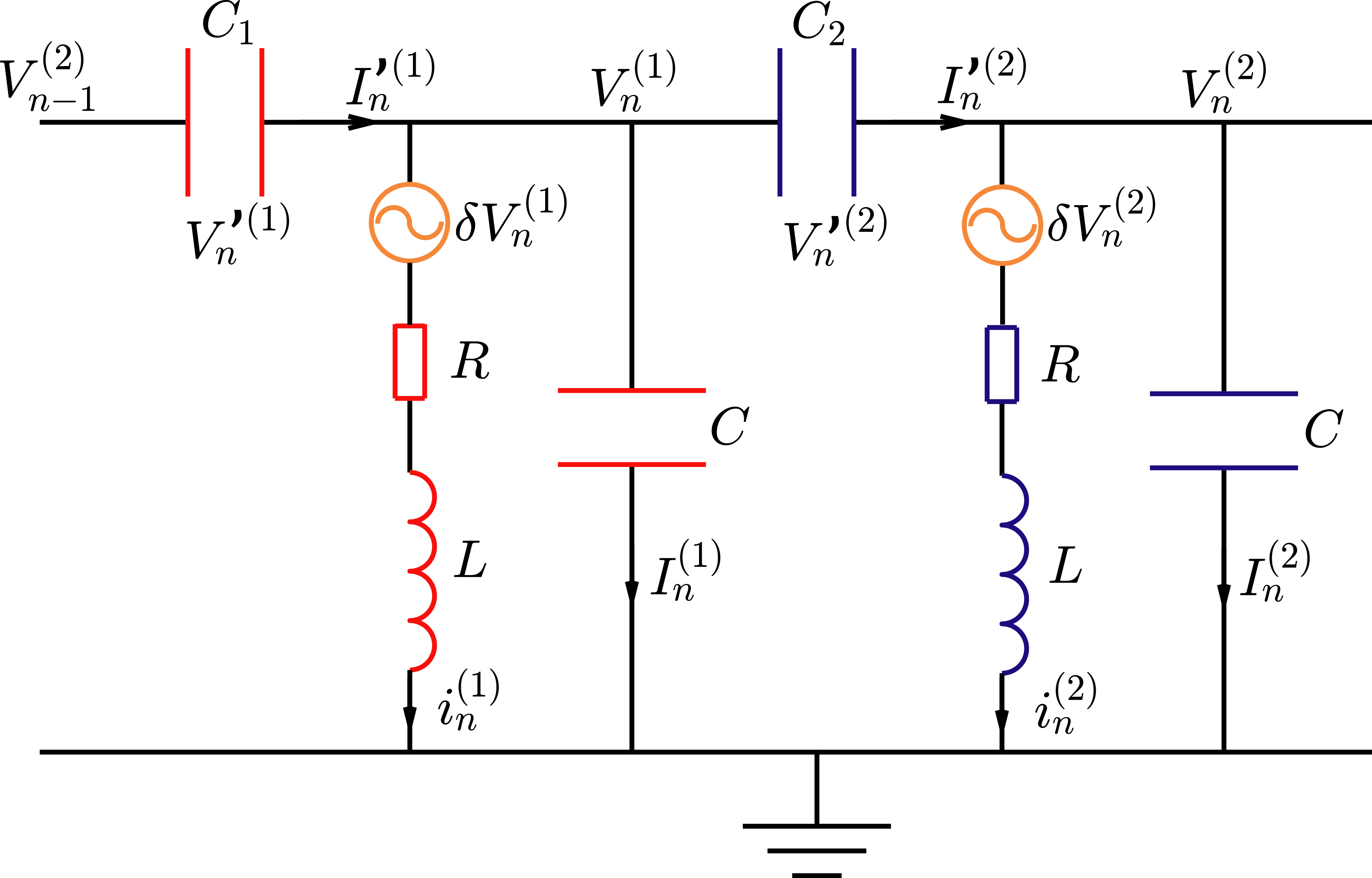
Here, we demonstrate that the equations of motion of 1D nonlinear topoelectrical LCR circuit can be converted to generalized nonlinear Schrödinger equations with the specific nonlinear interactions in Eq.(71). As shown in Fig.E1, the unit cell of the ladder circuit is composed of two resonators of natural frequency ω0=1/LC\omega_{0}=1/\sqrt{LC}, where LL is the inductance and CC is the capacitance. The resonators are connected by small capacitors Cj=1,2CC_{j=1,2}\ll C. We denote the voltages of the resonators as Vn(j)V_{n}^{(j)}, the currents of the inductances as in(j)i_{n}^{(j)}, and the currents of the capacitors as In(j)I_{n}^{(j)}. We further denote the voltages and currents of the nonlinear capacitors as Vn(j)V_{n}^{\prime(j)} and In(j)I_{n}^{\prime(j)}, respectively. Finally, external active sources δVn(j)\delta V_{n}^{(j)} as the nonlinear functions of Vn(j)V_{n}^{(j)} are internally installed in resonators. Kirchhoff’s law tells us

Vn(1)=Vn1(2)Vn(1),\displaystyle V_{n}^{\prime(1)}=V_{n-1}^{(2)}-V_{n}^{(1)},
Vn(2)=Vn(1)Vn(2),\displaystyle V_{n}^{\prime(2)}=V_{n}^{(1)}-V_{n}^{(2)},
In(1)=in(1)+In(1)+In(2),\displaystyle I_{n}^{\prime(1)}=i_{n}^{(1)}+I_{n}^{(1)}+I_{n}^{\prime(2)},
In(2)=in(2)+In(2)+In+1(1).\displaystyle I_{n}^{\prime(2)}=i_{n}^{(2)}+I_{n}^{(2)}+I_{n+1}^{\prime(1)}. (171)

We also have

In(j)=CV˙n(j),\displaystyle I_{n}^{(j)}=C\dot{V}_{n}^{(j)},
In(j)=CjV˙n(j),\displaystyle I_{n}^{\prime(j)}=C_{j}\dot{V}_{n}^{\prime(j)}, (172)

for j=1,2j=1,2. By adopting the limit of small capacitances Hadad et al. (2018) CjCC_{j}\ll C, from Eqs.(E.2, E.2) we obtain

in(1)\displaystyle i_{n}^{(1)} \displaystyle\approx C1V˙n1(2)+C2V˙n(2)CV˙n(1),\displaystyle C_{1}\dot{V}_{n-1}^{(2)}+C_{2}\dot{V}_{n}^{(2)}-C\dot{V}_{n}^{(1)},
in(2)\displaystyle i_{n}^{(2)} \displaystyle\approx C1V˙n+1(1)+C2V˙n(1)CV˙n(2).\displaystyle C_{1}\dot{V}_{n+1}^{(1)}+C_{2}\dot{V}_{n}^{(1)}-C\dot{V}_{n}^{(2)}. (173)

The equations of motion for the inductances are

Li˙n(j)+Rin(j)=Vn(j)δVn(j)=defUn(j).\displaystyle L\dot{i}_{n}^{(j)}+Ri_{n}^{(j)}=V_{n}^{(j)}-\delta V_{n}^{(j)}\overset{\rm def}{=}U_{n}^{(j)}. (174)

where δVn(j)Vn(j)\delta V_{n}^{(j)}\ll V_{n}^{(j)} is assumed here. Finally, we employ the approximation CjCC_{j}\ll C again to simplify Eq.(174) as follows,

V¨n(1)ω02+RCV˙n(1)=Un(1)C1CUn1(2)C2CUn(2),\displaystyle\frac{\ddot{V}_{n}^{(1)}}{\omega_{0}^{2}}+RC\dot{V}_{n}^{(1)}=-U_{n}^{(1)}-\frac{C_{1}}{C}U_{n-1}^{(2)}-\frac{C_{2}}{C}U_{n}^{(2)},
V¨n(2)ω02+RCV˙n(2)=Un(2)C1CUn+1(1)C2CUn(1).\displaystyle\frac{\ddot{V}_{n}^{(2)}}{\omega_{0}^{2}}+RC\dot{V}_{n}^{(2)}=-U_{n}^{(2)}-\frac{C_{1}}{C}U_{n+1}^{(1)}-\frac{C_{2}}{C}U_{n}^{(1)}.\qquad (175)

We note that Cj/C1C_{j}/C\ll 1, which means

CjCUn(j)CjCVn(j).\displaystyle\frac{C_{j}}{C}U_{n}^{(j^{\prime})}\approx\frac{C_{j}}{C}V_{n}^{(j^{\prime})}. (176)

Thus, Eqs.(E.2) further reduce to

V¨n(1)ω02+RCV˙n(1)=Vn(1)+δVn(1)C1CVn1(2)C2CVn(2),\displaystyle\frac{\ddot{V}_{n}^{(1)}}{\omega_{0}^{2}}+RC\dot{V}_{n}^{(1)}=-V_{n}^{(1)}+\delta V_{n}^{(1)}-\frac{C_{1}}{C}V_{n-1}^{(2)}-\frac{C_{2}}{C}V_{n}^{(2)},
V¨n(2)ω02+RCV˙n(2)=Vn(2)+δVn(2)C1CVn+1(1)C2CVn(1).\displaystyle\frac{\ddot{V}_{n}^{(2)}}{\omega_{0}^{2}}+RC\dot{V}_{n}^{(2)}=-V_{n}^{(2)}+\delta V_{n}^{(2)}-\frac{C_{1}}{C}V_{n+1}^{(1)}-\frac{C_{2}}{C}V_{n}^{(1)}.

We then express the voltages as the envelope function

Vn(j)=Ψn(j)eiω0t\displaystyle V_{n}^{(j)}=\Psi_{n}^{(j)}e^{-\mathrm{i}\omega_{0}t} (178)

which in turn gives us

V¨n(j)\displaystyle\ddot{V}_{n}^{(j)} =\displaystyle= (Ψ¨n(j)2iω0Ψ˙n(j)ω02Ψn(j))eiω0t\displaystyle(\ddot{\Psi}_{n}^{(j)}-2\mathrm{i}\omega_{0}\dot{\Psi}_{n}^{(j)}-\omega_{0}^{2}\Psi_{n}^{(j)})e^{-\mathrm{i}\omega_{0}t} (179)
\displaystyle\approx (2iω0Ψ˙n(j)ω02Ψn(j))eiω0t,\displaystyle(-2\mathrm{i}\omega_{0}\dot{\Psi}_{n}^{(j)}-\omega_{0}^{2}\Psi_{n}^{(j)})e^{-\mathrm{i}\omega_{0}t},

where in the second step we assume that the time-modulation of Vn(j)V_{n}^{(j)} is mostly captured by the factor eiω0te^{-\mathrm{i}\omega_{0}t} and hence Ψn(j)\Psi_{n}^{(j)} varies slowly in time, giving Ψ¨n(j)ω0Ψ˙n(j)\ddot{\Psi}_{n}^{(j)}\ll\omega_{0}\dot{\Psi}_{n}^{(j)}. We denote the damping coefficient η=RCω0/21\eta=RC\omega_{0}/2\ll 1 for simplicity. It is at this point that we obtain the equations of motion which is expressed as generalized nonlinear Schrödinger equations with small damping

(iη)Ψ˙n(1)+iηω0Ψn(1)=\displaystyle\left(\mathrm{i}-\eta\right)\dot{\Psi}_{n}^{(1)}+\mathrm{i}\eta\omega_{0}\Psi_{n}^{(1)}=
ω0C12CΨn1(2)+ω0C22CΨn(2)ω02eiω0tδVn(1),\displaystyle\frac{\omega_{0}C_{1}}{2C}\Psi_{n-1}^{(2)}+\frac{\omega_{0}C_{2}}{2C}\Psi_{n}^{(2)}-\frac{\omega_{0}}{2}e^{\mathrm{i}\omega_{0}t}\delta V_{n}^{(1)},
(iη)Ψ˙n(2)+iηω0Ψn(2)=\displaystyle\left(\mathrm{i}-\eta\right)\dot{\Psi}_{n}^{(2)}+\mathrm{i}\eta\omega_{0}\Psi_{n}^{(2)}=
ω0C12CΨn+1(1)+ω0C22CΨn(1)ω02eiω0tδVn(2).\displaystyle\frac{\omega_{0}C_{1}}{2C}\Psi_{n+1}^{(1)}+\frac{\omega_{0}C_{2}}{2C}\Psi_{n}^{(1)}-\frac{\omega_{0}}{2}e^{\mathrm{i}\omega_{0}t}\delta V_{n}^{(2)}. (180)

Having established the nonlinear Schrödinger equations, we now discuss how to realize the nonlinear interactions specified in Eq.(71). This can be achieved by asking

δVn(1)\displaystyle\delta V^{(1)}_{n} =\displaystyle= δc1Vn1(2)δc2Vn(2)\displaystyle-\delta c_{1}V_{n-1}^{(2)}-\delta c_{2}V_{n}^{(2)}
eiω0t{d1[(ReΨn1(2))3+i(ImΨn1(2))3]\displaystyle-e^{-\mathrm{i}\omega_{0}t}\bigg{\{}d_{1}\left[({\rm Re\,}\Psi_{n-1}^{(2)})^{3}+\mathrm{i}({\rm Im\,}\Psi_{n-1}^{(2)})^{3}\right]
+d2[(ReΨn(2))3+i(ImΨn(2))3]},\displaystyle+d_{2}\left[({\rm Re\,}\Psi_{n}^{(2)})^{3}+\mathrm{i}({\rm Im\,}\Psi_{n}^{(2)})^{3}\right]\bigg{\}},
δVn(2)\displaystyle\delta V^{(2)}_{n} =\displaystyle= δc1Vn+1(1)δc2Vn(1)\displaystyle-\delta c_{1}V_{n+1}^{(1)}-\delta c_{2}V_{n}^{(1)} (181)
eiω0t{d1[(ReΨn+1(1))3+i(ImΨn+1(1))3]\displaystyle-e^{-\mathrm{i}\omega_{0}t}\bigg{\{}d_{1}\left[({\rm Re\,}\Psi_{n+1}^{(1)})^{3}+\mathrm{i}({\rm Im\,}\Psi_{n+1}^{(1)})^{3}\right]
+d2[(ReΨn(1))3+i(ImΨn(1))3]}.\displaystyle+d_{2}\left[({\rm Re\,}\Psi_{n}^{(1)})^{3}+\mathrm{i}({\rm Im\,}\Psi_{n}^{(1)})^{3}\right]\bigg{\}}.
Refer to caption
Figure F1: Topological properties of nonlinear SSH lattice subjected to Kerr-type nonlinearities. The interaction parameters, including ϵ0\epsilon_{0}, c1c_{1}, c2c_{2}, d1d_{1} and d2d_{2}, are the same as those in Fig.1. (a) Nonlinear band structures for various amplitudes ranging from A=0A=0 to 1.2ac1.2a_{c}, where ac=(c2c1)/(d2d1)=0.7746a_{c}=\sqrt{-(c_{2}-c_{1})/(d_{2}-d_{1})}=0.7746. The nonlinear bands touch at the critical amplitude A=acA=a_{c}, and Berry phase changes abruptly from γ(A<ac)=π\gamma(A<a_{c})=\pi to γ(A>ac)=0\gamma(A>a_{c})=0. (b) By constructing a finite lattice shown in Fig.2(a) with open boundary conditions, we shake the boundary on site n=1n=1 by imposing a Gaussian tone burst in Eq.(131) to excite nonlinear topological modes, where S=6.5×10²S=6.5\times 10^{-2}, ωext=ϵ0=1.5\omega_{\rm ext}=\epsilon_{0}=1.5, T=2π/ωextT=2\pi/\omega_{\rm ext}, τ=3T\tau=3T, and t0=15Tt_{0}=15T. (c) Responding mode on n=1,2,3n=1,2,3 sites indicates the mode localization, where the mode amplitude max(ReΨ1(1))<ac\max({\rm Re\,}\Psi_{1}^{(1)})<a_{c}. (d) Brown and blue curves stand for the frequency spectra of external Gaussian signal and n=1n=1 site responding wave function. Yellow shaded area is the linear bandgap. (e) Spatial profile of the boundary excitation amplitude. We note that the bulk mode components reflected here are excited by Gaussian signal, which contains all frequencies. (f) Red and blue curves are the spatial profiles of the ω=ϵ0\omega=\epsilon_{0} Fourier component of the boundary mode. The analytic result of the ω=ϵ0\omega=\epsilon_{0} Fourier component is depicted by the black dashed curve. (g) The echo-like wave functions of sites n=10,20,30n=10,20,30 manifest bulk mode components excited by the external Gaussian shaking signal. (h) The spectrum of n=20n=20 site contains a wide range of frequency components of bulk modes. (i) We now study topological edge modes in the lattice depicted by Fig.D4(a), where the interaction parameters c1c_{1}^{\prime} and d1d_{1}^{\prime} of the defect bond at site n=7n=7 are carried over from that figure. Responding modes are plotted for n=1,2,3n=1,2,3 sites which exhibit the feature of mode localization. (j) Fourier analysis of frequency space for wave function at site n=1n=1. (k) Spatial profile of the responding amplitudes. A noticeable bump at site n=7n=7 is induced by the defect. (l) Spatial profile of the ω=ϵ0\omega=\epsilon_{0} frequency component is captured by red and blue curves, and the theoretical analysis of this component is described by the black dashed curve.

Appendix F An analytically solvable topological model with Kerr-type nonlinear interactions

We study an alternative model to provide additional verification of the nonlinear topological theory presented in this paper. The model is analytically solvable, in the sense that the nonlinear bulk modes as well as the dispersion relation can be exactly solved. The model is based on Eqs.(A) with the Kerr-type nonlinearities D’Aguanno et al. (2008) on the field variables,

fi(x,y)=ciy+di|y|2y,i=1,2,\displaystyle f_{i}(x,y)=c_{i}y+d_{i}|y|^{2}y,\quad i=1,2, (182)

where the parameters yield 0<c1<c20<c_{1}<c_{2} and d1>d2>0d_{1}>d_{2}>0. This model is subjected to reflection symmetry. According to the main text, reflection symmetry demands the quantization of Berry phase of nonlinear bulk modes, regardless of the functional forms of interactions. This conclusion should remain valid for Kerr-type nonlinearities. To verify the quantization of Berry phase, we solve nonlinear traveling modes as below,

Ψn=A(1,eiϕq)eiqniωt,\displaystyle\Psi_{n}=A(1,e^{-\mathrm{i}\phi_{q}})^{\top}e^{\mathrm{i}qn-\mathrm{i}\omega t}, (183)

where the dispersion relation is

ω=ϵ0±c1(A)2+c2(A)2+2c1(A)c2(A)cosq,\displaystyle\omega=\epsilon_{0}\pm\sqrt{c_{1}(A)^{2}+c_{2}(A)^{2}+2c_{1}(A)c_{2}(A)\cos q},\qquad (184)

ci(A)=ci+diA2c_{i}(A)=c_{i}+d_{i}A^{2}, and the relative phase ϕq\phi_{q} is

ϕq=arctan(c2(A)sinqc1(A)+c2(A)cosq).\displaystyle\phi_{q}=\arctan\left(\frac{-c_{2}(A)\sin q}{c_{1}(A)+c_{2}(A)\cos q}\right). (185)

Following the convention of Fourier transformation in Eq.(26), the Fourier components of the sinusoidal nonlinear bulk mode are ψl,q(1)=ψl,q(2)=Aδl,1\psi_{l,q}^{(1)}=\psi_{l,q}^{(2)}=A\delta_{l,1}. According to Eq.(184), the nonlinear bandgap never closes unless the wave amplitude hits the topological transition point aca_{c}. Apart from aca_{c}, Berry phase of nonlinear bulk modes is well-defined, and can be greatly simplified to the following result by employing the sinusoidal form of nonlinear waves,

γ(A)=12iBZdqqln[c1(A)+c2(A)eiq].\displaystyle\gamma(A)=\frac{1}{2}\mathrm{i}\oint_{\rm BZ}\mathrm{d}q\,\partial_{q}\ln[c_{1}(A)+c_{2}(A)e^{\mathrm{i}q}]. (186)

According to our general theory, Berry phase is expected to be γ(A<ac)=π\gamma(A<a_{c})=\pi and γ(A>ac)=0\gamma(A>a_{c})=0, which holds true for arbitrary reflection-symmetric 1D systems and is independent of the functional forms of nonlinearities. This result is verified by evaluating Eq.(186) for Kerr-type nonlinear interactions.

As stated by the nonlinear extension of bulk-boundary correspondence, nonlinear topological modes should emerge on the lattice open boundary when the bulk band is topologically non-trivial with Berry phase γ=π\gamma=\pi, whereas topological modes disappear when γ=0\gamma=0. Here we confirm this correspondence by studying the attributes of nonlinear topological edge modes. To this end, we Fourier transform the edge mode into frequency space, and truncating it to the fundamental harmonics,

Ψnψ1,neiωt+ψ1,neiωt.\displaystyle\Psi_{n}\approx\psi_{-1,n}e^{\mathrm{i}\omega t}+\psi_{1,n}e^{-\mathrm{i}\omega t}. (187)

Similarly, the nonlinear terms in the interactions are truncated as follows,

|Ψn(j)|2Ψn(j)\displaystyle|\Psi_{n}^{(j)}|^{2}\Psi_{n}^{(j)} \displaystyle\approx (|ψ1,n(j)|2+2|ψ1,n(j)|2)ψ1,n(j)eiωt\displaystyle(|\psi_{-1,n}^{(j)}|^{2}+2|\psi_{1,n}^{(j)}|^{2})\psi^{(j)}_{-1,n}e^{\mathrm{i}\omega t} (188)
+\displaystyle+ (2|ψ1,n(j)|2+|ψ1,n(j)|2)ψ1,n(j)eiωt.\displaystyle(2|\psi^{(j)}_{-1,n}|^{2}+|\psi^{(j)}_{1,n}|^{2})\psi^{(j)}_{1,n}e^{-\mathrm{i}\omega t}.

Consequently, the equations of motion reduce to the following nonlinear recursion relations,

(ϵ0sω)ψs,n(1)+C1(ψs,n(2))+C2(ψs,n1(2))=0,\displaystyle(\epsilon_{0}-s\omega)\psi_{s,n}^{(1)}+{C}_{1}(\psi_{s,n}^{(2)})+{C}_{2}(\psi_{s,n-1}^{(2)})=0,
(ϵ0sω)ψs,n(2)+C1(ψs,n(1))+C2(ψs,n+1(1))=0,\displaystyle(\epsilon_{0}-s\omega)\psi_{s,n}^{(2)}+{C}_{1}(\psi_{s,n}^{(1)})+{C}_{2}(\psi_{s,n+1}^{(1)})=0, (189)

where s=±1s=\pm 1, and

Ci(ψs,n(j))=ciψs,n(j)+di(|ψs,n(j)|2+2|ψs,n(j)|2)ψs,n(j).\displaystyle{C}_{i}(\psi_{s,n}^{(j)})=c_{i}\psi_{s,n}^{(j)}+d_{i}(|\psi^{(j)}_{s,n}|^{2}+2|\psi^{(j)}_{-s,n}|^{2})\psi^{(j)}_{s,n}.\qquad (190)

We exploit the approximation ψs,n(1)ψs,n(2)\psi^{(1)}_{s,n}\gg\psi^{(2)}_{s,n}, which is numerically verified in Fig.F1(f). We solve Eqs.(F) to find ω=ϵ0\omega=\epsilon_{0}, ψ1,n(1)=0\psi_{-1,n}^{(1)}=0 for all nn, Argψ1,n(1)=Argψ1,1(1)+(n1)π{\rm Arg\,}\psi_{1,n}^{(1)}={\rm Arg\,}\psi_{1,1}^{(1)}+(n-1)\pi, and

c1(ψ1,n(1))|ψ1,n(1)|=c2(ψ1,n+1(1))|ψ1,n+1(1)|,\displaystyle c_{1}(\psi_{1,n}^{(1)})|\psi_{1,n}^{(1)}|=c_{2}(\psi_{1,n+1}^{(1)})|\psi_{1,n+1}^{(1)}|, (191)

where ci(x)=ci+di|x|2c_{i}(x)=c_{i}+d_{i}|x|^{2}. Based on Eq.(191), when |ψ1,1(1)|<ac|\psi_{1,1}^{(1)}|<a_{c}, an evanescent mode fades away from the lattice boundary, whereas for |ψ1,1(1)|>ac|\psi_{1,1}^{(1)}|>a_{c}, an unphysical mode quickly diverges to infinity and therefore cannot exist. The emergence and disappearance of edge modes are in accordance with topologically non-trivial and trivial Berry phases, which is the manifestation of bulk-boundary correspondence with Kerr-type nonlinearities.

References

  • Haldane (1988) F. D. M. Haldane, Phys. Rev. Lett. 61, 2015 (1988).
  • Fu et al. (2007) L. Fu, C. L. Kane,  and E. J. Mele, Phys. Rev. Lett. 98, 106803 (2007).
  • Hasan and Kane (2010) M. Z. Hasan and C. L. Kane, Rev. Mod. Phys. 82, 3045 (2010).
  • Ryu et al. (2010) S. Ryu, A. P. Schnyder, A. Furusaki,  and A. W. Ludwig, New Journal of Physics 12, 065010 (2010).
  • Kane and Lubensky (2014) C. Kane and T. Lubensky, Nature Physics 10, 39 (2014).
  • Süsstrunk and Huber (2015) R. Süsstrunk and S. D. Huber, Science 349, 47 (2015).
  • Hadad et al. (2018) Y. Hadad, J. C. Soric, A. B. Khanikaev,  and A. Alù, Nature Electronics 1, 178 (2018).
  • Li et al. (2018) F. Li, X. Huang, J. Lu, J. Ma,  and Z. Liu, Nature Physics 14, 30 (2018).
  • Duncan et al. (2017) C. W. Duncan, P. Öhberg,  and M. Valiente, Phys. Rev. B 95, 125104 (2017).
  • Zhou and Zhang (2020) D. Zhou and J. Zhang, Phys. Rev. Research 2, 023173 (2020).
  • Vila et al. (2019) J. Vila, G. H. Paulino,  and M. Ruzzene, Phys. Rev. B 99, 125116 (2019).
  • Prodan and Prodan (2009) E. Prodan and C. Prodan, Phys. Rev. Lett. 103, 248101 (2009).
  • Ma et al. (2018) J. Ma, D. Zhou, K. Sun, X. Mao,  and S. Gonella, Phys. Rev. Lett. 121, 094301 (2018).
  • Smirnova et al. (2020) D. Smirnova, D. Leykam, Y. Chong,  and Y. Kivshar, Applied Physics Reviews 7, 021306 (2020).
  • Li et al. (2014) F. Li, P. Anzel, J. Yang, P. G. Kevrekidis,  and C. Daraio, Nature communications 5, 1 (2014).
  • Nash et al. (2015) L. M. Nash, D. Kleckner, A. Read, V. Vitelli, A. M. Turner,  and W. T. Irvine, Proceedings of the National Academy of Sciences 112, 14495 (2015).
  • Zhou et al. (2018) D. Zhou, L. Zhang,  and X. Mao, Phys. Rev. Lett. 120, 068003 (2018).
  • Luo et al. (2021) L. Luo, H.-X. Wang, Z.-K. Lin, B. Jiang, Y. Wu, F. Li,  and J.-H. Jiang, Nature Materials , 1 (2021).
  • Zhou et al. (2019) D. Zhou, L. Zhang,  and X. Mao, Phys. Rev. X 9, 021054 (2019).
  • Lo et al. (2021) P.-W. Lo, K. Roychowdhury, B. Gin-ge Chen, C. D. Santangelo, C.-M. Jian,  and M. J. Lawler, arXiv e-prints , arXiv:2104.12778 (2021), arXiv:2104.12778 [cond-mat.soft] .
  • Zheng et al. (2020) W. Zheng, Q.-L. Lei, F. Tang, X. Wan, R. Ni,  and Y. Ma, arXiv e-prints , arXiv:2012.01639 (2020), arXiv:2012.01639 [cond-mat.soft] .
  • Hadad et al. (2016) Y. Hadad, A. B. Khanikaev,  and A. Alù, Phys. Rev. B 93, 155112 (2016).
  • Chaunsali and Theocharis (2019) R. Chaunsali and G. Theocharis, Phys. Rev. B 100, 014302 (2019).
  • Pal et al. (2018) R. K. Pal, J. Vila, M. Leamy,  and M. Ruzzene, Phys. Rev. E 97, 032209 (2018).
  • Zak (1989) J. Zak, Phys. Rev. Lett. 62, 2747 (1989).
  • Van Kampen (1992) N. G. Van Kampen, Stochastic processes in physics and chemistry, Vol. 1 (Elsevier, 1992).
  • Meerson (1996) B. Meerson, Rev. Mod. Phys. 68, 215 (1996).
  • Chen et al. (2014) B. G.-g. Chen, N. Upadhyaya,  and V. Vitelli, Proceedings of the National Academy of Sciences 111, 13004 (2014).
  • Zhou et al. (2020) D. Zhou, J. Ma, K. Sun, S. Gonella,  and X. Mao, Phys. Rev. B 101, 104106 (2020).
  • Crawford (1991) J. D. Crawford, Rev. Mod. Phys. 63, 991 (1991).
  • Su et al. (1979) W. P. Su, J. R. Schrieffer,  and A. J. Heeger, Phys. Rev. Lett. 42, 1698 (1979).
  • Eckmann and Ruelle (1985) J. P. Eckmann and D. Ruelle, Rev. Mod. Phys. 57, 617 (1985).
  • Altmann et al. (2013) E. G. Altmann, J. S. E. Portela,  and T. Tél, Rev. Mod. Phys. 85, 869 (2013).
  • Scalora et al. (2005) M. Scalora, M. S. Syrchin, N. Akozbek, E. Y. Poliakov, G. D’Aguanno, N. Mattiucci, M. J. Bloemer,  and A. M. Zheltikov, Phys. Rev. Lett. 95, 013902 (2005).
  • Lazarides and Tsironis (2005) N. Lazarides and G. P. Tsironis, Phys. Rev. E 71, 036614 (2005).
  • Narisetti et al. (2010) R. K. Narisetti, M. J. Leamy,  and M. Ruzzene, Journal of Vibration and Acoustics 132 (2010).
  • Zaera et al. (2018) R. Zaera, J. Vila, J. Fernandez-Saez,  and M. Ruzzene, International Journal of Non-Linear Mechanics 106, 188 (2018).
  • Vakakis et al. (2001) A. F. Vakakis, L. I. Manevitch, Y. V. Mikhlin, V. N. Pilipchuk,  and A. A. Zevin, Normal modes and localization in nonlinear systems (Springer, 2001).
  • Fronk and Leamy (2017) M. D. Fronk and M. J. Leamy, Journal of Vibration and Acoustics 139 (2017).
  • Leggett (2001) A. J. Leggett, Rev. Mod. Phys. 73, 307 (2001).
  • Xiao et al. (2010) D. Xiao, M.-C. Chang,  and Q. Niu, Rev. Mod. Phys. 82, 1959 (2010).
  • Liu et al. (2003) J. Liu, B. Wu,  and Q. Niu, Phys. Rev. Lett. 90, 170404 (2003).
  • Pu et al. (2007) H. Pu, P. Maenner, W. Zhang,  and H. Y. Ling, Phys. Rev. Lett. 98, 050406 (2007).
  • Liu and Fu (2010) J. Liu and L. B. Fu, Phys. Rev. A 81, 052112 (2010).
  • Renson et al. (2016) L. Renson, G. Kerschen,  and B. Cochelin, Journal of Sound and Vibration 364, 177 (2016).
  • Ha (2001) S. N. Ha, Computers & Mathematics with Applications 42, 1411 (2001).
  • Peeters et al. (2008) M. Peeters, R. Viguié, G. Sérandour, G. Kerschen,  and J.-C. Golinval, in 26th International Modal Analysis Conference, Orlando, 2008 (2008).
  • Shang et al. (2018) C. Shang, Y. Zheng,  and B. A. Malomed, Phys. Rev. A 97, 043602 (2018).
  • Detroux et al. (2014) T. Detroux, L. Renson,  and G. Kerschen, in Nonlinear Dynamics, Volume 2 (Springer, 2014) pp. 19–34.
  • Snee and Ma (2019) D. D. Snee and Y.-P. Ma, Extreme Mechanics Letters 30, 100487 (2019).
  • D’Aguanno et al. (2008) G. D’Aguanno, N. Mattiucci,  and M. J. Bloemer, JOSA B 25, 1236 (2008).
  • Christodoulides and Joseph (1988) D. N. Christodoulides and R. I. Joseph, Opt. Lett. 13, 794 (1988).
  • Benalcazar et al. (2017) W. A. Benalcazar, B. A. Bernevig,  and T. L. Hughes, Science 357, 61 (2017).
  • Luther (1968) H. Luther, Mathematics of Computation 22, 434 (1968).