Topological Floquet engineering of a three-band optical lattice with dual-mode resonant driving

Let us consider a spinless fermionic atom in the driven 1D optical lattice potential $V_{\rm lat}(x,t)$, which is given by

where $V_{L}(t)$ and $\phi(t)$ are the amplitude and phase of the lattice potential, respectively, and $a$ is the lattice constant. $V_{L}$ and $\phi$ are determined by the parameters of the laser beams involved, such as intensity, polarization, and phase, and can be dynamically controlled for Floquet engineering. The two fundamental modulation approaches are periodically modulating $V_{L}$ and $\phi$ in time, which we refer to as AM and PM, respectively [Figs. 1(b) and 1(c)]. As the position of the lattice site is determined by the phase $\phi(t)$, PM induces lattice shaking. When viewed from the reference frame comoving with the driven optical lattice, the system’s Hamiltonian is described as follows [5, 9]:

where $p$ is the kinetic momentum of the atom, $m$ denotes its mass, $V_{\rm stat}(x)=V_{0}\sin^{2}\left(\frac{\pi}{a}x\right)$ is the stationary lattice potential, $\lambda(t)$ denotes the relative variation of lattice amplitude such that $V_{L}(t)=[1+\lambda(t)]V_{0}$, and $F(t)=-m\left(\frac{a}{\pi}\ddot{\phi}(t)\right)$ represents the inertial force resulting from PM.

In the tight-binding approximation, the Hamiltonian can be expressed in terms of Wannier states $|j,\alpha\rangle$ localized on lattice site $j$ in the $\alpha$ band, given by [9]

where $\hat{c}^{{\dagger}}_{j\alpha}\,(\hat{c}_{j\alpha})$ is the creation (annihilation) operator for the atom in the Wannier state $|j,\alpha\rangle$, $\epsilon_{\alpha}=\langle j,\alpha|H_{0}|j,\alpha\rangle$ represents the on-site energy, and $t^{(l)}_{\alpha}=-\langle j,\alpha|H_{0}|j+l,\alpha\rangle$ denotes the hopping amplitude between the Wannier states in the $\alpha$ band separated by $l$ lattice sites. In addition, $u^{(l)}_{\alpha\beta}=\langle j,\alpha|V_{\rm stat}(x)|j+l,\beta\rangle$ and $\eta^{(l)}_{\alpha\beta}=\langle j,\alpha|x|j+l,\beta\rangle$ correspond to the lattice potential and lattice displacement matrix elements for interorbital transitions separated by $l$ lattice sites, respectively. Lastly, $\theta(t)=-\frac{a}{\hbar}\int_{0}^{t}dt^{\prime}\,F(t^{\prime})$ represents the time-dependent Peierls phase [40]. See Appendix A for detailed definitions of the tight-binding parameters. By Fourier transforming this tight-binding model Hamiltonian, we obtain the Bloch Hamiltonian for quasimomentum $q$ in the presence of AM and PM as follows:

Here, $q$ is expressed in units of $1/a$.

In this work, we consider a model system that includes only the three lowest bands, indexed by $\alpha\in\{s,p,d\}$. Considering the lowest-order effects of lattice modulation, the Bloch Hamiltonian of the three-band system is given by

with $\epsilon_{\alpha}^{\prime}(q,t)=\epsilon_{\alpha}-2t^{(1)}_{\alpha}\cos(q-\theta(t))+\lambda(t)u^{(0)}_{\alpha\alpha}$. See Appendix A for details on the derivation.

We focus on a case where the system is subjected to dual-mode resonant driving with

and the driving frequency $\omega\approx\omega_{sd}=(\epsilon_{d}-\epsilon_{s})/\hbar$. Here, $\lambda_{0}$ and $\phi_{0}$ are dimensionless parameters that represent the strengths of AM and PM, respectively, and $\varphi$ is the relative phase of the two modulation modes.

When the three-band lattice system is driven with a frequency $\omega\approx\omega_{sd}$, the couplings between the $p$ orbital and the others become off-resonant, resulting in the $p$ band being energetically isolated. We can project the three-band system into an effective two-band system using an adiabatic elimination technique [39] owing to the minimal involvement of the $p$ band in band mixing.

First, let us take a proper rotating frame by applying a unitary transformation of $U_{R}(t)=\exp{(+i\hat{R}t)}$ to the Bloch Hamiltonian $H(q,t)$ in Eq. (5), where

with $E_{0}=(\epsilon_{d}+\epsilon_{s}+\hbar\omega)/2$ representing the zero energy point. In the rotating frame, the modified Hamiltonian $H^{\prime}(q,t)$ is given by

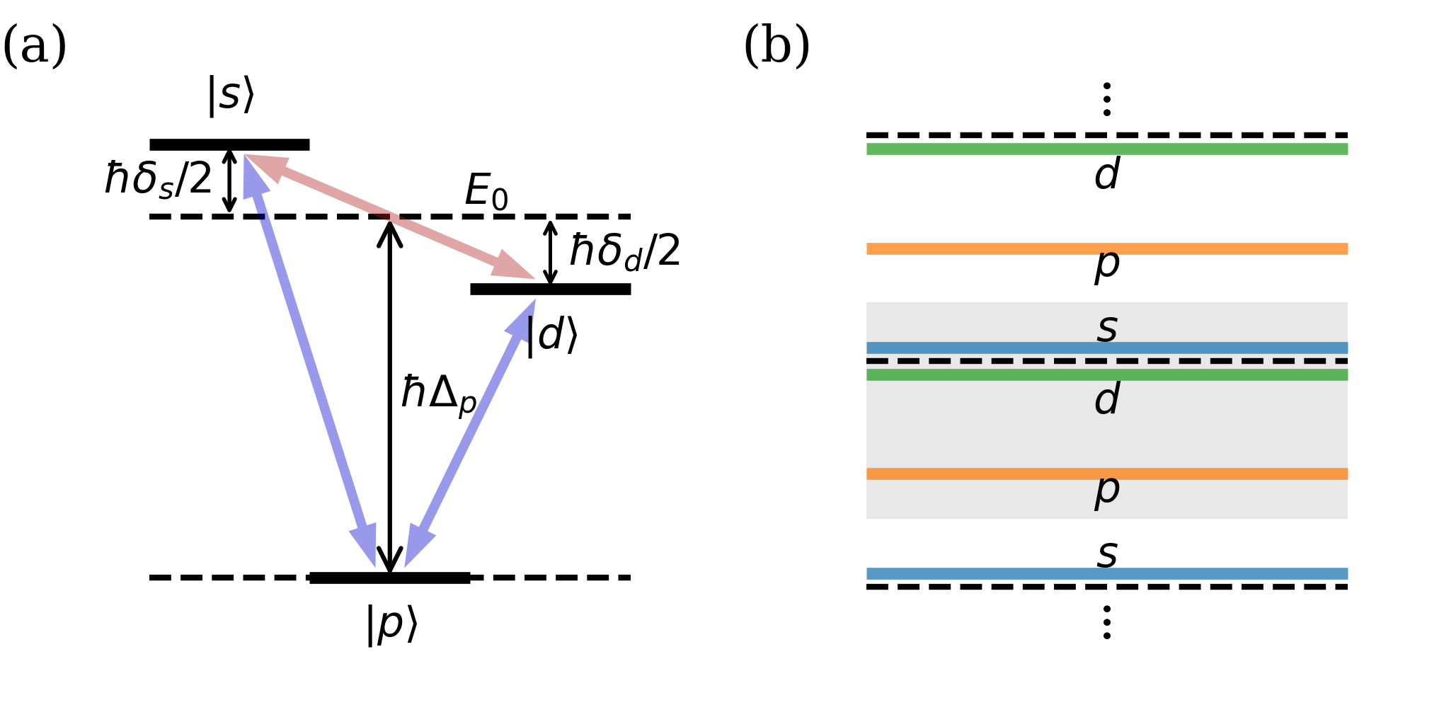
with $\hbar\delta_{s}/2=\epsilon_{s}^{\prime}+\hbar\omega-E_{0}$, $\hbar\delta_{d}/2=E_{0}-\epsilon_{d}^{\prime}$, and $\hbar\Delta_{p}=E_{0}-\epsilon_{p}^{\prime}$. Note that $|\Delta_{p}|\gg|\delta_{s}|,|\delta_{d}|$ when the driving frequency is set to $\omega\approx\omega_{sd}$, providing a suitable condition for adiabatic elimination of the $p$ band. The energy level structure is depicted in Fig. 2(a). It can be viewed as a characteristic V-type system in which the two adjacent upper states are coupled to each other by $\lambda(t)$ and also to a lower level simultaneously by $F(t)$. For comparison, the Floquet energy diagram of the driven three-band system is illustrated in Fig. 2(b).

Simplifying the notation of $H^{\prime}(q,t)$ as

the equation of motion for the system state $|\psi\rangle=(\rho_{s},\rho_{p},\rho_{d})^{\text{T}}$ is written by

Claiming $\dot{\rho}_{p}=0$ owing to the $p$ band being negligibly populated, we obtain $\rho_{p}=-(H_{10}\rho_{s}+H_{12}\rho_{d})/H_{11}$. Injecting this relation back into Eq. (II.2) yields the effective Hamiltonian as

The additional terms in the diagonal and the off-diagonal element are proportional to $\frac{F^{2}}{\Delta_{p}}$, which represent additive band energy shifts and $sd$ interband couplings, respectively, arising from the off-resonant couplings to the $p$ band.

In terms of the Pauli matrices $\bm{\sigma}=\{\sigma_{x},\sigma_{y},\sigma_{z}\}$, we obtain the modified effective Hamiltonian as

with $\delta=\omega-\omega_{sd}$. The definitions of $t_{-}$, $\theta_{0}$, $\lambda^{\prime}_{(-)}$, and $F^{\prime}_{(-)}$ are listed in Table 1. In the derivation of $H_{\rm eff}^{\prime}$, we ignored the trace part of the Hamiltonian, i.e., $H_{\rm eff}^{\prime}=H_{\rm eff}-\frac{{\rm tr}(H_{\rm eff})}{2}\mathbb{I}$, which does not affect the topological properties of the system.

Next, we derive the approximated time-independent Hamiltonian $\tilde{H}_{\rm eff}(q)$ for $H_{\rm eff}^{\prime}(q,t)$ using the high-frequency expansion method [41, 42]. When the Fourier series expansion of $H_{\rm eff}^{\prime}(q,t)$ is given by $H_{\rm eff}^{\prime}(q,t)=\Sigma_{m}H_{m}(q)e^{im\omega t}$, the second-order approximation of $\tilde{H}_{\rm eff}(q)$ is given by

Neglecting the higher order terms [43], we obtain

where $\delta^{\prime}=\hbar\delta/2-{F^{\prime}_{-}}^{2}$, $t^{\prime}_{-}=t_{-}J_{0}(\theta_{0})$, $t_{v}=\lambda^{\prime}/2$, and $t_{d}=\frac{3{F^{\prime}}^{2}}{\hbar\omega}t_{-}J_{1}(\theta_{0})$. The details of the derivation are provided in Appendix B.

The final expression of $\tilde{H}_{\rm eff}(q)$ in Eq. (II.2) reveals the band topology of the driven lattice system. The terms with $t_{v}$ and $t_{d}$ correspond to the vertical and diagonal interleg links in the two-leg-ladder description [Fig. 1(a)]. Notably,

indicating that the vertical links are generated by the on-site one-photon interorbital transition $|j,s\rangle\leftrightarrow|j,d\rangle$, induced by AM, while the diagonal links originate from the three-photon transitions involving site hopping, e.g., $|j,s\rangle\leftrightarrow|j,p\rangle\leftrightarrow|j,d\rangle\leftrightarrow|j+1,d\rangle$, induced by PM.

The effective Hamiltonian $\tilde{H}_{\rm eff}(q)$ exhibits chiral symmetry at $\varphi=\pm\frac{\pi}{2}$, as $\sigma_{y}\tilde{H}_{\rm eff}(q)\sigma_{y}=-\tilde{H}_{\rm eff}(q)$; this means that the spin states of the bands are restricted to the $xz$ plane of a three-dimensional space with axes represented by Pauli matrices, ensuring that the spin winding number across the Brillouin zone is well-defined and topologically protected by symmetry. At $\delta^{\prime}=0$, a topologically critical point emerges when $t_{d}=\pm t_{v}/2$, rendering $\tilde{H}_{\rm eff}(q=\mp\frac{\pi}{2})=0$ for $\varphi=\frac{\pi}{2}$ and $\tilde{H}_{\rm eff}(q=\pm\frac{\pi}{2})=0$ for $\varphi=-\frac{\pi}{2}$. Given the parameters of the optical lattice system at $V_{0}=10\,E_{R}$ ($E_{R}$ is the lattice recoil energy), as detailed in Table 1, the ratio $|t_{v}/t_{d}|=2$ is achieved when ${\phi_{0}}^{3}/{\lambda_{0}}=0.009$. This modulation condition is experimentally feasible, for example, with $\lambda_{0}=0.1$ and $\phi_{0}\approx 0.1$, which corresponds to the lattice-shaking amplitude of $0.03a$.

Thus far, we have demonstrated that a cross-linked ladder structure can be established in a three-band optical lattice by utilizing dual-mode resonant driving. Developing an effective two-band description, we have clarified the critical role of the off-resonant $p$ band in Floquet engineering, which is essential for determining the topological characteristics of the driven lattice system. In the following section, we will confirm our theoretical findings through a direct numerical simulation of the three-band Hamiltonian $H(q,t)$ in Eq. (5).

We investigate the quasienergy spectrum of the driven three-band optical lattice system in accordance with Floquet theory [44]. We numerically calculate the time-evolution operator over one driving period $T=\frac{2\pi}{\omega}$, defined as

with $\mathcal{T}$ being the time-ordering operator, and obtain the quasienergy spectrum $\varepsilon_{n}(q)$ by directly diagonalizing $\hat{U}(t+T,t;q)$. Here, $n=0,1,2$ is the Floquet band index and $\varepsilon_{n}(q)\in[-\frac{\hbar\omega}{2},\frac{\hbar\omega}{2})$ is independent of the choice of time $t$. In the calculation, we use the parameter values listed in Table 1 and set the modulation frequency to $\omega=\omega_{sd}$.

In Fig. 3(a), the quasienergy spectrum is presented for $\lambda_{0}=0.05$, $\phi_{0}=0.1$, and $\varphi=0$. The two upper ($n=1,2$) Floquet bands demonstrate the avoided crossing of the bare $s$ and $d$ bands of the stationary lattice system under the resonant driving, while the lower ($n=0$) Floquet band is located apart from the upper bands, aligned with the off-resonant $p$ band. In Figs. 3(b)–3(d), we plot the fractional weights of the $\alpha=s,p,d$ orbitals in the Floquet Bloch states $|\psi_{n}(q,t)\rangle$. The Floquet Bloch states are eigenstates of $\hat{U}(t+T,t;q)$ such that

It is observed that the $p$ orbital contribution is minimal in the upper Floquet bands, as expected from the off-resonance nature of the $p$ band. This observation supports the validity of our use of adiabatic elimination in the previous section.

To examine the topological characteristics of the driven lattice system, we calculate the Zak phases of the Floquet bands [45, 46], which are defined over the Brillouin zone (BZ) as

The numerical results of $\gamma_{n}(t=0)$ for $\phi_{0}=0.1$ are illustrated in Fig. 4, as a function of the driving parameters $\lambda_{0}$ and $\varphi$. It is noted that critical points are found at $\lambda_{0}=0.082$ and $\varphi=\pm\frac{\pi}{2}$, accompanied by discontinuous changes in $\gamma_{1}$ and $\gamma_{2}$ nearby. The effective two-band model in the previous section predicts the critical points at $\lambda_{0}=0.071$ for $\delta=0$ and $\phi_{0}=0.1$, which is in a good agreement with our numerical observations [47]. We note that when $\varphi=\pm\frac{\pi}{2}$, the Zak phase takes only the values of zero or $\pi$, while the Zak phase continuously varies in the parameter space; this is consistent with the symmetry protection condition discussed in the previous section. Furthermore, we observe that $\gamma_{1}+\gamma_{2}=0$ only for $\varphi=\pm\frac{\pi}{2}$, i.e., the Zak phase of the lowest $(n=0)$ Floquet band is $\gamma_{0}\neq 0$ for $\varphi\neq\pm\frac{\pi}{2}$ [Fig. 4(c)]; this is a characteristic of a three-band system.

In Fig. 4(d), we show the time evolution of the Zak phases for $\varphi=\frac{\pi}{2}$, revealing that they show quantized values only at $t=0$ and $\frac{T}{2}$. For the effective two-band Floquet system, the chiral symmetry is expressed as $\sigma_{y}{H_{\rm eff}}^{\prime}(q,t+t_{0})\sigma_{y}=-{H_{\rm eff}}^{\prime}(q,-t+t_{0})$ with a proper choice of time frame $t_{0}$ [6], and we find that the symmetry condition is satisfied only with $\varphi=\pm\frac{\pi}{2}$ (mod $2\pi$) at $t_{0}=0$ and $\frac{T}{2}$ (mod $T$), which is consistent with the times when the Zak phases are well quantized.

As another topological characteristic of the system, we examine the entanglement entropy and spectrum [28, 29, 30, 31, 32, 33]. For a 1D non-interacting fermionic system, the entanglement entropy $S$ of the many-body ground state $|\Psi\rangle$ is defined as

where $\rho_{\rm A}={\rm Tr}_{\rm B}|\Psi\rangle\langle\Psi|$ is the reduced density matrix of $|\Psi\rangle$ on subsystem A. Here, A and B denote the two subsystems that are formed by splitting the system into two equal parts. The entanglement spectrum $\xi$ comprises the eigenvalues of the single-particle correlation matrix, $C^{lm}_{jk}=\langle\Psi|\hat{a}^{{\dagger}}_{jl}\hat{a}_{km}|\Psi\rangle$, limited to subsystem A, where $\hat{a}^{{\dagger}}_{jl}\,(\hat{a}_{jl})$ denotes the creation (annihilation) operator for an atom in the Floquet Wannier state $|j,l\rangle$, localized on lattice site $j$ within subsystem A in the $n=l$ Floquet band. The details on the calculation of $S$ and $\xi$ are provided in Appendix D. When the system undergoes a quantum phase transition, the entanglement entropy exhibits a sharp peak [33] and furthermore, the entanglement spectrum unveils the system’s mid-gap states. The presence of mid-gap states serves as an indication of the non-trivial topological phase of the system, which is analogous to the bulk-edge correspondence observed in edge states [29, 30], and it holds even in the case of Floquet systems [31, 32].

Figure 5 presents our calculation results of the entanglement entropy and spectrum of non-interacting spinless fermions for our three-band system. The many-body ground state $|\Psi\rangle$ is a uniformly filled topological Floquet band, and we choose the $n=1$ band in Fig. 3(a) as our reference state. When $\varphi=\pi/2$, the entanglement entropy exhibits a sharp peak at the critical point as $\lambda_{0}$ varies [Fig. 5(a)], indicating a topological phase transition [29, 32]. In the entanglement spectrum, we also observe the presence of mid-gap states and their splitting into upper and lower states at the same critical point of $\lambda_{0}$ [Fig. 5(b)]. These results are consistent with the Zak phase in the parameter space [Fig. 4(b)].

Finally, we remark on the edge states in our system, which are another characteristic of the topological phase [48, 49]. In our three-band system, the global bulk gap may not exist because both the $s$ and $d$ bands exhibit a similar curvature tendency, although varying in degree. The absence of the global bulk gap implies that symmetry-protected edge states may not manifest explicitly, which was the case in our numerical investigation.

When the driving parameters {$\lambda_{0},\varphi$} vary slowly enough compared to the timescale of the driving period $T$, the system can adiabatically follow the change in driving conditions. In other words, the long-term dynamics of the system is governed by the time-varying effective Hamiltonian, $H_{\text{eff}}(q;t)=H_{\text{eff}}(q;\{\lambda_{0},\varphi\})$ [50, 51]. Using this adiabatic following, topological charge pumping can be achieved in a driven lattice system by slowly varying the driving parameters around a topological singular point, as demonstrated in recent experiments [13, 16].

Given its experimental relevance, we numerically investigate the topological charge pumping effect in the driven three-band system. A pumping protocol is considered, where the driving parameters slowly revolve around a singular point in the parameter space with the pumping cycle time $T_{p}$, i.e.,

with $\varphi_{0}=\pi/2$. The system undergoes a $2\pi$ change in the Zak phase for each cycle, leading to a charge transport in which all atoms are shifted by one lattice site. Note that this phenomenon only occurs when the trajectory of the driving parameters encircles the singular point in the parameter space, regardless of the specific details of the pumping protocol used to modulate the driving parameters [34, 35, 36, 37, 38]; this is why this charge pumping phenomenon is a topological one.

In the numerical simulation, the system is initially prepared in an insulating state of the Flquet band and the amount of pumped charge is calculated as $C(t)=\int_{0}^{t}dt^{\prime}j(t^{\prime})$, where $j(t)$ is the charge current given by $j(t)=\frac{1}{2\pi}\int_{\text{BZ}}\langle\psi(q,t)|v(q,t)|\psi(q,t)\rangle$ with velocity operator $v(q,t)=\partial H(q,t)/\partial(\hbar q)$ [52, 53]. The time evolution of the system state $|\psi(q,t)\rangle$ is calculated directly from its time-dependent Shrödinger equation $i\partial_{t}|\psi(q,t)\rangle=H(q,t)|\psi(q,t)\rangle$, including the cyclic modulations of the driving parameters.

In Fig. 6(a), the pumped charge $C(t)$ is displayed as a function of time for various pumping parameter conditions. We observe that when the change of driving parameters is slow enough, $C(t)$ increases (decreases) by unity in every pumping cycle for the $n=2$ ($n=1$) Floquet band. The observed timescale for the adiabaticity of the charge pumping process is $T_{p}\approx 100T$, attributed to the local gap between the $n=1$ and $n=2$ Floquet bands, estimated as $\approx 0.01\hbar\omega$ [Fig. 3(a)]. Furthermore, we confirm that if the trajectory of the driving parameters, such as the case of $\varphi_{0}=0$ in Eq. (III.3), does not encircle any topological singular point in the parameter space, then the charge transport does not occur [Fig. 6(b)]. The middle inset of Fig. 6(a) shows the evolution of the entanglement spectrum of the driven lattice system during one pumping cycle, $T_{p}$. As expected, the mid-gap states propagate like edge modes in the bulk gap [54, 53].

References

- [1] M. Aidelsburger, M. Atala, M. Lohse, J. T. Barreiro, B. Paredes, and I. Bloch, Realization of the Hofstadter Hamiltonian with Ultracold Atoms in Optical Lattices, Phys. Rev. Lett. 111, 185301 (2013).
- [2] G. Jotzu, M. Messer, R. Desbuquois, M. Lebrat, T. Uehlinger, D. Greif, and T. Esslinger, Experimental realization of the topological haldane model with ultracold fermions, Nature 515, 237 (2014).
- [3] N. Goldman, J. C. Budich, and P. Zoller, Topological quantum matter with ultracold gases in optical lattices, Nat. Phys. 12, 639 (2016).
- [4] A. Eckardt, Colloquium: Atomic quantum gases in periodically driven optical lattices, Rev. Mod. Phys. 89, 011004 (2017).
- [5] N. R. Cooper, J. Dalibard, and I. B. Spielman, Topological bands for ultracold atoms, Rev. Mod. Phys. 91, 015005 (2019).
- [6] T. Kitagawa, E. Berg, M. Rudner, and E. Demler, Topological characterization of periodically driven quantum systems, Phys. Rev. B 82, 235114 (2010).
- [7] P. Hauke, O. Tieleman, A. Celi, C. Ölschläger, J. Simonet, J. Struck, M. Weinberg, P. Windpassinger, K. Sengstock, M. Lewenstein, and A. Eckardt, Non-Abelian Gauge Fields and Topological Insulators in Shaken Optical Lattices, Phys. Rev. Lett. 109, 145301 (2012).
- [8] J. Cayssol, B. Dóra, F. Simon, and R. Moessner, Floquet topological insulators, Phys. Status Solidi 7, 101 (2013).
- [9] N. Goldman and J. Dalibard, Periodically driven quantum systems: Effective hamiltonians and engineered gauge fields, Phys. Rev. X 4, 031027 (2014).
- [10] W. Zheng and H. Zhai, Floquet topological states in shaking optical lattices, Phys. Rev. A 89, 061603(R) (2014).
- [11] L. D. Marin Bukov and A. Polkovnikov, Universal high-frequency behavior of periodically driven systems: from dynamical stabilization to floquet engineering, Adv. Phys. 64, 139 (2015).
- [12] J. H. Kang, J. H. Han, and Y. Shin, Creutz ladder in a resonantly shaken 1D optical lattice, New J. Phys. 22, 013023 (2020).
- [13] J. Minguzzi, Z. Zhu, K. Sandholzer, A.-S. Walter, K. Viebahn, and T. Esslinger, Topological Pumping in a Floquet-Bloch Band, Phys. Rev. Lett. 129, 053201 (2022).
- [14] Y.-P. Wu, L.-Z. Tang, G.-Q. Zhang, and D.-W. Zhang, Quantized topological anderson-thouless pump, Phys. Rev. A 106, L051301 (2022).
- [15] R. Citro and M. Aidelsburger, Thouless pumping and topology, Nat. Rev. Phys. 5, 87 (2023).
- [16] A.-S. Walter, Z. Zhu, M. Gächter, J. Minguzzi, S. Roschinski, K. Sandholzer, K. Viebahn, and T. Esslinger, Quantization and its breakdown in a hubbard–thouless pump, Nat. Phys. 19, 1471 (2023).
- [17] M. Creutz, End States, Ladder Compounds, and Domain-Wall Fermions, Phys. Rev. Lett. 83, 2636 (1999).
- [18] D. Hügel and B. Paredes, Chiral ladders and the edges of quantum hall insulators, Phys. Rev. A 89, 023619 (2014).
- [19] J. Jünemann, A. Piga, S.-J. Ran, M. Lewenstein, M. Rizzi, and A. Bermudez, Exploring interacting topological insulators with ultracold atoms: The synthetic creutz-hubbard model, Phys. Rev. X 7, 031057 (2017).
- [20] K. Sandholzer, A.-S. Walter, J. Minguzzi, Z. Zhu, K. Viebahn, and T. Esslinger, Floquet engineering of individual band gaps in an optical lattice using a two-tone drive, Phys. Rev. Res. 4, 013056 (2022).
- [21] S.-L. Zhang and Q. Zhou, Shaping topological properties of the band structures in a shaken optical lattice, Phys. Rev. A 90, 051601(R) (2014).
- [22] J. H. Kang and Y. Shin, Topological floquet engineering of a one-dimensional optical lattice via resonant shaking with two harmonic frequencies, Phys. Rev. A 102, 063315 (2020).
- [23] C. Sträter and A. Eckardt, Interband heating processes in a periodically driven optical lattice, Z. Naturforsch. A 71, 909 (2016).
- [24] C. Cabrera-Gutiérrez, E. Michon, M. Arnal, G. Chatelain, V. Brunaud, T. Kawalec, J. Billy, and D. Guéry-Odelin, Resonant excitations of a bose einstein condensate in an optical lattice, Eur. Phys. J. D 73, 170 (2019).
- [25] A. A. Burkov, Topological semimetals, Nat. Mater. 15, 1145 (2016).
- [26] K. Sun, W. V. Liu, A. Hemmerich, and S. Das Sarma, Topological semimetal in a fermionic optical lattice, Nat. Phys. 8, 67 (2012).
- [27] M. Jangjan and M. V. Hosseini, Topological phase transition between a normal insulator and a topological metal state in a quasi-one-dimensional system, Sci. Rep. 11, 12966 (2021).
- [28] H. Li and F. D. M. Haldane, Entanglement Spectrum as a Generalization of Entanglement Entropy: Identification of Topological Order in Non-Abelian Fractional Quantum Hall Effect States, Phys. Rev. Lett. 101, 010504 (2008).
- [29] A. M. Turner, Y. Zhang, and A. Vishwanath, Entanglement and inversion symmetry in topological insulators, Phys. Rev. B 82, 241102(R) (2010).
- [30] T. L. Hughes, E. Prodan, and B. A. Bernevig, Inversion-symmetric topological insulators, Phys. Rev. B 83, 245132 (2011).
- [31] D. J. Yates, Y. Lemonik, and A. Mitra, Entanglement properties of floquet-chern insulators, Phys. Rev. B 94, 205422 (2016).
- [32] L. Zhou, Entanglement spectrum and entropy in floquet topological matter, Phys. Rev. Res. 4, 043164 (2022).
- [33] S. Ryu and Y. Hatsugai, Entanglement entropy and the berry phase in the solid state, Phys. Rev. B 73, 245115 (2006).
- [34] D. J. Thouless, Quantization of particle transport, Phys. Rev. B 27, 6083 (1983).
- [35] L. Wang, M. Troyer, and X. Dai, Topological Charge Pumping in a One-Dimensional Optical Lattice, Phys. Rev. Lett. 111, 026802 (2013).
- [36] F. Mei, J.-B. You, D.-W. Zhang, X. C. Yang, R. Fazio, S.-L. Zhu, and L. C. Kwek, Topological insulator and particle pumping in a one-dimensional shaken optical lattice, Phys. Rev. A 90, 063638 (2014).
- [37] S. Nakajima, T. Tomita, S. Taie, T. Ichinose, H. Ozawa, L. Wang, M. Troyer, and Y. Takahashi, Topological thouless pumping of ultracold fermions, Nat. Phys. 12, 296 (2016).
- [38] M. Lohse, C. Schweizer, O. Zilberberg, M. Aidelsburger, and I. Bloch, A thouless quantum pump with ultracold bosonic atoms in an optical superlattice, Nat. Phys. 12, 350 (2016).
- [39] E. Brion, L. H. Pedersen, and K. Mølmer, Adiabatic elimination in a lambda system, J. Phys. A 40, 1033 (2007).
- [40] M. Weinberg, C. Ölschläger, C. Sträter, S. Prelle, A. Eckardt, K. Sengstock, and J. Simonet, Multiphoton interband excitations of quantum gases in driven optical lattices, Phys. Rev. A 92, 043621 (2015).
- [41] S. Rahav, I. Gilary, and S. Fishman, Effective hamiltonians for periodically driven systems, Phys. Rev. A 68, 013820 (2003).
- [42] A. Eckardt and E. Anisimovas, High-frequency approximation for periodically driven quantum systems from a floquet-space perspective, New J. Phys. 17, 093039 (2015).
- [43] We ignore the terms with the second order Bessel function and the higher order terms of and .
- [44] M. Holthaus, Floquet engineering with quasienergy bands of periodically driven optical lattices, J. Phys. B 49, 013001 (2015).
- [45] J. Zak, Berry’s phase for energy bands in solids, Phys. Rev. Lett. 62, 2747 (1989).
- [46] M. Z. Hasan and C. L. Kane, Colloquium: Topological insulators, Rev. Mod. Phys. 82, 3045 (2010).
- [47] Different from the case when , where the gap closes at , in this instance, the gap closing occurs at due to the presence of the energy shift which results in .
- [48] M. Mancini, G. Pagano, G. Cappellini, L. Livi, M. Rider, J. Catani, C. Sias, P. Zoller, M. Inguscio, M. Dalmonte, and L. Fallani, Observation of chiral edge states with neutral fermions in synthetic hall ribbons, Science 349, 1510 (2015).
- [49] B. K. Stuhl, H.-I. Lu, L. M. Aycock, D. Genkina, and I. B. Spielman, Visualizing edge states with an atomic bose gas in the quantum hall regime, Science 349, 1514 (2015).
- [50] V. Novičenko, E. Anisimovas, and G. Juzeliūnas, Floquet analysis of a quantum system with modulated periodic driving, Phys. Rev. A 95, 023615 (2017).
- [51] P. Weinberg, M. Bukov, L. D’Alessio, A. Polkovnikov, S. Vajna, and M. Kolodrubetz, Adiabatic perturbation theory and geometry of periodically-driven systems, Phys. Rep. 688, 1 (2017).
- [52] N. Sun and L.-K. Lim, Quantum charge pumps with topological phases in a creutz ladder, Phys. Rev. B 96, 035139 (2017).
- [53] D. Xiao, M.-C. Chang, and Q. Niu, Berry phase effects on electronic properties, Rev. Mod. Phys. 82, 1959 (2010).
- [54] R. Resta, Manifestations of berry’s phase in molecules and condensed matter, J. Phys. Condens. Matter 12, R107 (2000).
- [55] J. Ahn and B.-J. Yang, Unconventional Topological Phase Transition in Two-Dimensional Systems with Space-Time Inversion Symmetry, Phys. Rev. Lett. 118, 156401 (2017).
- [56] J. Ahn, D. Kim, Y. Kim, and B.-J. Yang, Band Topology and Linking Structure of Nodal Line Semimetals with Monopole Charges, Phys. Rev. Lett. 121, 106403 (2018).
- [57] Q. Wu, A. A. Soluyanov, and T. Bzdušek, Non-Abelian band topology in noninteracting metals, Science 365 1273 (2019).
- [58] J. Ahn, S. Park, D. Kim, Y. Kim, and B.-J. Yang, Stiefel–whitney classes and topological phases in band theory, Chin. Phys. B 28, 117101 (2019).
- [59] A. Bouhon, A. M. Black-Schaffer, and R.-J. Slager, Wilson loop approach to fragile topology of split elementary band representations and topological crystalline insulators with time-reversal symmetry, Phys. Rev. B 100 195135 (2019).
- [60] In [55, 58], symmetry is called space-time inversion symmetry.
- [61] C.-K. Chiu, J. C. Y. Teo, A. P. Schnyder, and S. Ryu, Classification of topological quantum matter with symmetries, Rev. Mod. Phys. 88, 035005 (2016).
- [62] R. Roy and F. Harper, Periodic table for floquet topological insulators, Phys. Rev. B 96, 155118 (2017).
- [63] S. A. Weidinger and M. Knap, Floquet prethermalization and regimes of heating in a periodically driven, interacting quantum system, Sci. Rep. 7, 45382 (2017).
- [64] M. S. Rudner and N. H. Lindner, Band structure engineering and non-equilibrium dynamics in Floquet topological insulators, Nat. Rev. Phys. 2, 229 (2020).