Topological conditions for impurity effects in carbon nanosystems

From the discovery, 20 years ago, of single-layer graphene Geim2004 , an enormous interest has been attracted not only to its two-dimensionality (2D) Geim2005 but mainly to its massless, that is Dirac-like, spectrum of electronic excitations Geim2009 . Studies of its various physical properties have a very broad nomenclature Tomanek_Book ; Inagaki2014 (see also Katsnelson ) but we focus here on certain aspects of non-ideal graphene structures, yet restricted to a single dimension (1D), namely, of graphene nanoribbons (NR’s) Wakabayashi2010 and carbon nanotubes (NT’s) Iijima2002 ; Charlier2007 in presence of impurities Nevidomskyy ; Jalili ; Pumera ; Skrypnyk ; Vejpravova . Mostly, we consider here the electron quasiparticle spectra in principal topological types of graphene 1D nanosystems and their restructuring under effects by impurity atoms absorbed at different positions over carbon atoms Wehling2009 ; Araujo . In this course, the main attention is given to the cases when Dirac-like 1D modes are present in the NT spectrum Wakabayashi1996 and we compare the impurity disorder effects on such modes with those previously studied in 2D graphene YDV2021 and in armchair type nanoribbons (ANR’s) PL2022 . Also, the specifics of impurity effects in more general twisted carbon NT’s are shortly discussed. The main purpose of this analysis is in finding possibile practical applications for such 1D-like semi-metallic systems under thier properly adjusted doping as more compact and sensible analogues for common doped semiconductors.

The presentation is organized as follows. We begin from description of quasiparticle spectra for two basic NT topologies: zigzag (ZNT’s, Sec. II) and armchair (ANT’s, Sec. III), in the forms adjusted to describe the impurity induced restructuring of their spectra. This description, within the simplest T-matrix approximation for the quasi-particle self-energy, begins from the technically simpler ANT case (Sec. IV) and then extends to a more involved ZNT case (Sec. V). The next comparison with the previous results for 2D graphene and ANR’s (Sec. VI) reveals both qualitative similarities and some quantitative differences in their behaviors. At least, the general topology of twisted nanotubes (TNT’s) is discussed in Sec. VII, suggesting a qualitative difference between the twisted and non-twisted NT’s in their sensitivity to impurity disorder. The obtained results are then verified with some T-matrix improvements (Sec. VIII): the self-consistent T-matrix method and the group expansion (GE) method, both of them confirming validity of the simple T-matrix picture. The final discussion of these theoretical results and of some perspectives for their practical applications is given in Sec. IX.

Carbon NT’s can be obtained from carbon NR’s by closure of their edges (for instance, of basic zigzag or armchair types), and these nanotubes are usually classified by the normals to their axes (that is to the related NR edges). Thus, folding of an armchair nanoribbon (ANR) produces a ZNT and, vice versa, that of a zigzag nanoribbon (ZNR) does an ANT.

Beginning from the ANR case, it can be seen as a composite of $n$ chains (labeled by $j$ indices) of transversal period $a$ (the graphene lattice constant), each chain containing $N\gg 1$ segments (labeled by $p$ indices) of longitudinal period $a\sqrt{3}$ and each segment including 4 atomic sites (labeled by $s$ indices, see Fig. 1).

Next, the closure between the 1st and $n$th chains of an ANR, transforms it into a ZNT (see Fig. 2).

For the following consideration of electronic dynamics, it is suitable to combine the local Fermi operators $a_{p,j,s}$ at 4 $s$-sites from $j$th chain in $p$th segment into the 4-spinor:

Then the longitudinal translation invariance (with the $a\sqrt{3}$ period, see Fig. 1) and the discrete transversal rotation invariance of the obtained ZNT suggest the Fourier expansion of the local spinor components in quasi-continuous longitudinal momentum $-\pi/\sqrt{3}<k<\pi/\sqrt{3}$ and in discrete transversal wave number $q=0,\dots,n-1$ (both in $a^{-1}$ units):

Its components $\alpha_{k,q,s}$ form the wave spinor $\alpha_{k,q}$. Here the longitudinal numbers for different $s$-sites are: $p_{1,2}=p\pm 1/6$, $p_{3,4}=p\pm 1/3$ and their transversal numbers are: $j_{1,2}=j$, $j_{3,4}=j+1/2$. Then the ZNT Hamiltonian with only account of hopping between nearest neighbor atoms (its parameter, $t\approx 2.8$ eV Geim2009 , taken as the energy scale in what follows) is presented in terms of wave spinors as ¹¹1The common nearest neighbor hopping approximation stays practically insensible to the NT curvature at $n\gg 1$ since the distance to next-nearest neighbors there stays, within to $\sim 1/n^{2}$, the same as in 2D graphene.:

Here the $4\times 4$ matrix:

has its elements $h_{k}={\rm e}^{ik/\sqrt{3}}$ and $h_{k,q}=2{\rm e}^{ik/2\sqrt{3}}\cos\tfrac{\pi q}{n}$. The ZNT spectrum results from four eigen-values of this matrix at given $k$ and $q$ as:

with the basic dispersion law:

This can be seen either as the standard graphene dispersion law Wallace but with discrete transversal momentum numbers $q$ or, otherwise, as a set of $4n$ 1D $k$-bands $\varepsilon_{k,q;f}$ (for $n$ possible values of $q$ and 4 values of $f$). Notably, a double degeneracy of these bands follows from Eqs. 5, 6 as:

Thus, if $n$ is even, the ZNT spectrum has 4 non-degenerated (for $q=0$ and $q=n/2$) modes and $2n-2$ doubly-degenerated ones. Otherwise, if $n$ is odd, there are two non-degenerated modes (only for $q=0$) and $2n-1$ doubly-degenerated ones. The eigen-operators $\psi_{k,q;f}$ of these modes enter the diagonal ANT Hamiltonian:

These operators at given $k$ and $q$ can be also combined into the 4-spinor $\psi_{k,q}$, related to the $\alpha$-spinor as:

through the unitary matrix:

with the complex phase factor

Contrariwise, the $\alpha$-spinor follows from the $\psi$-spinor by the inversion of Eq. 9:

Another important features of the ZNT spectrum by Eq. 5 are:

i) presence of 2 flat (dispersionless) modes for even $n$ (then at $q=n/2$) and

ii) presence of 4 gapless Dirac-like modes (DLM’s) for $n$ being a multiple of 3 (then at $q=n/3$ and $q=2n/3$).

The latter are just the 1D analogs to the 2D graphene Dirac modes with their nodal points $K$ (here at $k=2\pi/\sqrt{3},\,q=n/3$) and $K^{\prime}$ (here at $k=0,\,q=2n/3$), also they are fully analogous to DLM’s in ANR PL2022 .

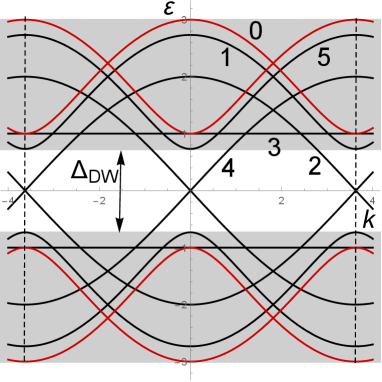
Due to the DLM’s special sensitivity to local impurity perturbations, our following treatment is mainly focused on these modes. In this course, the most relevant energy range is the Dirac window (DW), exclusively occupied with DLM’s and delimited by the inner edges of their nearest neighbor modes (Fig. 3). From Eq. 6, this window results of width:

and with growing $n\gg 1$ it is narrowing as $\sim 2\sqrt{3}\pi/n$.

Now, considering the low-energy spectrum range, the expansion of local operators by Eqs. 2, 10 can be restricted to 8 $K,K^{\prime}$ DLM’s which share 4 eigen-energies:

Thus, the restricted expansion of a local spinor in eigen-spinors is presented in the form:

including the unitary matrices:

with $z_{k}={\rm e}^{ik/2\sqrt{3}}$. This expansion is suitable for the following construction of impurity perturbation Hamiltonian.

For the case of ANT we also consider its structure obtained from an $n$-chain ZNR (Fig. 4) by closure between its 1st and $n$th chains (Fig. 5).

Comparison of Fig. 4 with Fig. 1 readily shows that the ANT elementary cell results just from 90 degrees rotation of the ZNT one, so the analysis of ANT spectra simply follows that for ZNT but with the $\sqrt{3}k\longleftrightarrow 2\pi q/n$ interchange. Thus the ANT Hamiltonian in terms of 4-spinor wave operators results, in analogy with the ZNT form by Eq. 2, as:

where the $4\times 4$ matrix:

has its elements $h_{q}={\rm e}^{i2\pi q/3n}$ and $h_{q,k}=2{\rm e}^{i\pi q/3n}\cos k/2$. The ANT spectrum at given $k$ and $q$ results from the indicated interchange in Eqs. 5, 6, as:

where:

This spectrum includes the same numbers of non-degenerated and doubly degenerated eigen-modes as in the above considered ZNT case. But it differs from that case by:

i) absence of flat modes and

ii) presence of two Dirac nodal points: $k=2\pi/3$ ($K$) and $k=-2\pi/3$ ($K^{\prime}$) at the same $q=0$ and for any ANT width $n$ value. Notably, the related two DLM’s are non-degenerated (compare with Eq. 12):

For the ANT case, the DW width results $\Delta_{\rm DW}=2\sin\pi/n$, that is narrowing with $n\gg 1$ as $\Delta_{\rm DLM}\sim 2\pi/n$ (to be compared with the ZNT case by Eq. 11).

It should be also noted that, unlike a complete similarity between the ZNT and ANR spectra, there is an important difference between those for ANT and ZNR (the latter having no DLM’s at all but presenting instead a special edge mode Nakada1996 , PL2022 ).

Then the expansion of local operators (an analog to Eq. 13), reduced to only DLM eigen-operators, results as:

with 2-spinors:

Due to relative simplicity of expansions by Eq. 29 in only 2 DLM’s, compared to the ZNT case by Eq. 13 with up to 8 DLM’s, we begin the next consideration of impurity effects just from the ANT case.

Now we can consider impurity effects on the above described NT’s. The simplest Lifshitz isotopic perturbation model Lifshitz is known not to produce impurity resonance effects in NR’s, both in ANR and ZNR PL2022 , therefore we begin from the more effective Anderson hybrid model Anderson , presenting its perturbation Hamiltonian for the ANT case (with use of 2-spinors by Eq. 29) as:

It describes impurity adatoms with their resonance energy $\varepsilon_{res}$ (laying inside the host DLM range) and corresponding local Fermi operators $b_{\sigma}$ at random positions $\sigma$, linked through the hybridization parameter $\gamma$ to its nearest neighbor host atom at $s_{\sigma}$ site in $p_{\sigma}$ segment of $j_{\sigma}$ chain (see Fig. 7). The random $p_{\sigma}$, $j_{\sigma}$, and $s_{\sigma}$ values are distributed uniformly with a low overall concentration: $c=(4nN)^{-1}\sum_{\sigma}1\ll 1$.

The next consideration goes in terms of (advanced) Green’s functions (GF’s) whose Fourier-transform in energy:

includes the grand-canonical statistical average: $\langle O\rangle={\rm Tr}\,\left[{\rm e}^{-(H-\mu)/k_{\mathrm{B}}T}O_{H}(t)\right]\bigl{/}\,{\rm Tr}\,\left[{\rm e}^{-(H-\mu)/k_{\mathrm{B}}T}\right]$ of a Heisenberg operator $O(t)={\rm e}^{iHt}O{\rm e}^{-iHt}$ under a Hamiltonian $H$ with chemical potential $\mu$ and the anticommutator $\{.,.\}$.

As known Zubarev1960 ; Economou1979 , GF’s satisfy the equation of motion:

In what follows the energy sub-index at GF’s is mostly omitted (or enters directly as its argument).

Consider now the GF $2\times 2$ matrix $\hat{G}(k,k^{\prime})=\langle\langle\psi_{k}|\psi_{k^{\prime}}^{\dagger}\rangle\rangle$ made of $\psi$-spinors by Eq. 29. In absence of impurities, with use of the Hamiltonian $H$ by Eq. 3, the explicit solution for this GF turns $k$-diagonal: $\hat{G}(k,k^{\prime})\to\delta_{k,k^{\prime}}\hat{G}^{(0)}(k)$, where

with the Pauli matrix $\hat{\tau}_{3}$.

When passing to the disordered system with its Hamiltonian extended to $H+H_{\rm AZ}$, we get the equation of motion for the $k$-diagonal GF matrix, $\hat{G}(k,k)\equiv\hat{G}(k)$:

and then its solution is generally sought in the self-energy form:

including the self-energy matrix $\hat{\Sigma}_{k}$. To find it, we continue the chain of equations of motion, now for the mixed (impurity-DLM) row-vector GF:

This gives the first contribution to $\hat{\Sigma}_{k}$ from its term with $k^{\prime}=k$ used in Eq. 42:

It is then extended by writing down the equation of motion for the resting terms with $k^{\prime}\neq k$ in the r.h.s. of Eq. 44:

and choosing the term with $\sigma^{\prime}=\sigma$ in its r.h.s. This generates the (scalar) impurity self-energy $\Sigma_{0}=\gamma^{2}G_{0}$ with the DLM locator GF:

which enters the modified factor $(\varepsilon-\varepsilon_{res}-\Sigma_{0})$ in Eq. 44. Then the solution for $\hat{G}(k)$ in the simplest T-matrix approximation for self-energy reads:

with the scalar T-matrix:

The next important GF, the DLM locator, is calculated by usual passing from $k$-summation to integration:

Its analytic expression (see Appendix) is:

approximated in the low-energy range as:

More generally, the DLM locator is defined as

with the diagonal GF matrix $\hat{G}(k)$ by Eq. 43. Within the T-matrix approximation by Eq. 48, it results simply as:

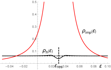
with $\tilde{\varepsilon}=\varepsilon-cT(\varepsilon)$ used instead of $\varepsilon$ in Eqs. 51 or 52. The resulting $G(\varepsilon)$ real and imaginary parts as shown in Fig. 8 for the choice of Cu impurities with $\varepsilon_{res}=0.03$, $\gamma=0.3$ Irmer2018 and $c=0.08$ only slightly differ from those for unperturbed $G_{0}(\varepsilon)$ within the $|\varepsilon-\varepsilon_{res}|\lesssim\gamma^{2}|G_{0}|$ range.

Another set of elementary excitations in the disordered system, that due to impurity atoms, defines the impurity locator GF: $G_{imp}=N^{-1}\sum_{\sigma}\langle\langle b_{\sigma}|b_{\sigma}^{\dagger}\rangle\rangle$, and its solution in the same approximation reads:

Together, the DLM and impurity locators, Eqs. 54, 55, define the low-energy density of states (DOS) as $\rho(\varepsilon)=\rho_{h}(\varepsilon)+\rho_{imp}(\varepsilon)$ with its host and impurity parts:

(taking the account of 2 spin values).

In a disordered ANT, host DLM’s contribute with $1/n$ charge carriers per site and impurities do with $c$ carriers per site, so defining the Fermi level $\varepsilon_{\rm F}$ from the equation:

(integrated from the bottom of DLM range). Then, in the simplest approximation of Im$G(\varepsilon)\approx{\rm Im}G_{0}(\varepsilon)\approx 2/(\sqrt{3}\pi n)$ (dashed line in Fig. 9), the Fermi level dependence on impurity concentration $c$ results:

where $c_{\ast}=[\gamma G_{0}(\varepsilon_{res})]^{2}$. Its fast initial growth: $\varepsilon_{\rm F}(c)\approx(c/c_{\ast})\varepsilon_{res}$ at $c\lesssim c_{\ast}$, changes to a slow approach of $\varepsilon_{res}$: $\varepsilon_{\rm F}(c)\approx\varepsilon_{res}-(c_{\ast}/c)\varepsilon_{res}$ at $c\gtrsim c_{\ast}$ (see Fig. 10).

The next analysis of low energy spectra in this disordered system follows the lines of similar cases by Refs. ILP1987 ; Pogorelov2020 ; PL2022 . Thus, the modified dispersion laws are obtained from the standard equation Bonch :

which splits in two scalar equations:

They appear as cubic equations for energy in function of momentum, $\varepsilon(k)$, and their analytic solutions, though standard, are rather cumbersome. But they can be greatly simplified within the relevant low energy range by using the linearized dispersion law:

with momentum $k$ referred to the Dirac point and Fermi velocity $\sqrt{3}/2$, and solving Eq. 60 for this momentum in function of energy PL2022 :

An example of such solutions for ANT with $n=12$ and $c=0.08$ in Fig. 11 demonstrates how coupling of each $\pm\varepsilon_{k}$ mode to the impurity $\varepsilon_{res}$ mode forms resonance splitting of hybridized $\pm\varepsilon_{1k}$ and $\pm\varepsilon_{2k}$ modes at $k=0$ to the interval of $\approx\sqrt{\varepsilon_{res}^{2}+4c\gamma^{2}}$ around $\varepsilon_{res}/2$.

Next, this $k_{\varepsilon}$-form is used in the important test of dispersion law validity for a disordered system, the Ioffe-Regel-Mott (IRM) criterion IoffeRegel ; Mott :

with the quasiparticle group velocity $v_{\varepsilon}=(\partial k_{\varepsilon}/\partial\varepsilon)^{-1}$ and its inverse lifetime $\tau_{\varepsilon}^{-1}=c\,{\rm Im}\,T(\varepsilon)$, that is the quasiparticle mean free path to be longer of its wavelength.

Each $\varepsilon$ value that converts $\gtrsim$ into $\approx$ in Eq. 63 gives an estimate for a mobility edge $\varepsilon_{mob}$, separating the ranges of band-like and localized states in the spectrum. An important rule for these states in a multi-mode system is that they can not coexist, that is, if, for a certain energy, the IRM criterion does not hold for at least one mode, all other modes at this energy should be also localized Mott .

With use of Eqs. 62, 49, such equation for mobility edges can be written explicitly in the form:

with $D^{2}(\varepsilon)=(\varepsilon-\varepsilon_{res})^{2}+\Gamma^{2}$ and $\Gamma=\gamma^{2}G_{0}(\varepsilon)$. Then, using the $G_{0}(\varepsilon)$ value by Eq. 51, this equation can be solved numerically to estimate all possible $\varepsilon_{mob}$ values and so delimit the band-like and localized energy ranges in ZNT with impurities at given disorder parameters ($\varepsilon_{res}$, $\gamma$, $c$) and of NT structure ($n$) as shown in Fig. 11.

Here one localized range is found at the lower limit of resonance splitting, near the shifted Dirac energy $-\varepsilon_{s}$ at all $c>0$, being of width $\approx c\gamma^{2}/\varepsilon_{res}$. Another localized range emerges above it, around $\varepsilon_{res}$, when $c$ reaches a certain critical value $c_{0}$. And at yet higher critical concentration, $c_{1}\gg c_{0}$, the latter range gets split in two, due to a specific interplay (when going away from the Dirac point) between the growing momentum $k_{\varepsilon}$, decreasing group velocity $v_{k}$, and increasing inverse lifetime $\tau_{\varepsilon}^{-1}$ of hybridized modes. A more detailed description of these restructured spectra for different nanostructures follows below.

It is also of interest to extend the above approach to another NT topology, namely, to the more involved ZNT case. To simplify description of low energy impurity resonances here, we again restrict the expansions of local operators by Eqs. 2 and 9 in 4-spinors $\psi(k,q)$ with unitary matrices $\hat{U}(k,q)$, to only DLM’s $q=K,K^{\prime}$. Then the ZNT perturbation Hamiltonian results, instead of Eq. 38 for ZNT, in the form:

where the row spinor $u^{\dagger}(k,q;\sigma)$ is just the $j_{\sigma}$-th row of $\hat{U}^{\dagger}(k,q)$.

Next we consider the 4$\times$4 GF matrices $\hat{G}(k,q;k^{\prime},q^{\prime})\equiv\langle\langle\psi_{k,q}|\psi_{k^{\prime},q^{\prime}}^{\dagger}\rangle\rangle$ and the related equation of motion with the Hamiltonian $H+H_{\rm Z}$ for the choice of $K$-modes GF:

where $G_{f,f^{\prime}}^{(0)}(k,K)=\delta_{f,f^{\prime}}(\varepsilon-\varepsilon_{k,K,f})^{-1}$ and the column spinor $u(k,q;\sigma)$ is the $j_{\sigma}$-th column of $\hat{U}(k,q)$.

Then the equation (similar to Eq. 44 for the ZNT case) for the mixed GF, $\langle\langle b_{\sigma}|\psi_{k^{\prime},K}^{\dagger}\rangle\rangle$:

leads (in the same way as to Eq. 48) to the T-matrix solution for momentum-diagonal GF matrix $\hat{G}(k,K)\equiv\hat{G}(k,K;k,K)$:

where the T-function for this case differs from that by Eq. 49 only by the form of its locator $G_{0}(\varepsilon)$. Using Eq. 12, it results here as:

Then comparison with Eq. 51 shows that the impurity level damping for this case turns $\approx 8\sqrt{3}$ times stronger than for ANT at the same $n$ number, mostly due to the above indicated greater relative weight of DLM’s in ZNT than in ANT spectra. This produces strongly different behaviors of IRM mobility edges and qualitatively different structures of localized and band-like spectra in these two nanosystems.

The low-energy spectrum restructuring under impurity disorder effect is suitably illustrated by a diagram of mobility edges $\varepsilon_{mob}$ between the localized and band-like energy ranges in function of impurity concentration $c$. Such diagrams in Fig. 12 permit to compare the effects of Cu impurities on Dirac modes in the previously considered 2D graphene Pogorelov2020 and ANRs PL2022 together with the above obtained results for ZNT and ANT.

Some general features, noted for the ANT case, are observed in all of them: i) formation of a localized range (mobility gap) around the resonance level $\varepsilon_{res}$, at reaching a certain critical concentration $c_{0}$, ,

ii) presence of another localized range around the shifted down Dirac level $\varepsilon_{D}$, being mostly narrower but existing at all $c>0$,

iii) opening, at a certain higher critical concentration $c_{1}\gg c_{0}$, of a narrow band range within the $\varepsilon_{res}$-related mobility gap.

But this comparison also reveals notably different sensitivity of the corresponding DLM’s to the impurity resonance level, depending both on their topological properties (absence or presence of edges and the edge types) and on discrete transversal numbers of chains in a system. Within the IRM formalism, for given impurity parameters $\varepsilon_{res}$ and $\gamma$, it depends on the host system through its locator function $G_{0}(\varepsilon)$, like those by Eqs. 51, 69. This can be further compared with the previously found $G_{0}(\varepsilon)$ values for 2D graphene: $\varepsilon/\sqrt{3}$ YDV2021 and for ANR with $M$ carbon chains: $4/(M+1)$ PL2022 .

Thus, the impurity-induced localization first occurs at an energy very close to $\varepsilon_{res}$ and the related critical concentration $c_{0}$ can be estimated from Eq. 64 by setting $\varepsilon=\varepsilon_{res}$ there. It results generally in:

and for the instance of ANT with $n=12$ it gives $c_{0}\approx 1.7\cdot 10^{-4}$ in a reasonable agreement with the numerical calculation result shown in Fig. 12. With further growth of $c>c_{0}$, a continuous range of localized states (mobility gap) appears around $\varepsilon_{res}$, of width growing as $\Delta_{mob}\sim\gamma\sqrt{c-c_{0}}$.

Then, at reaching another critical concentration $c_{1}\gg c_{0}$, a certain window of band-like states opens inside the mobility gap, due to the before discussed faster resonance splitting between the initial $\varepsilon_{k}$ and $\varepsilon_{res}$ modes than these split modes damping. This $c_{1}$ value is also estimated from the numerical solution of IRM Eq. 63. It can be presented in function of the single $G_{0}$ parameter as shown in Fig. 13. Strictly speaking, this is only possible for 1D nanosystems where the low-energy locator $G_{0}(\varepsilon)$ is practically constant, defined by their topology and discrete width numbers. This dependence can be reasonably fitted by the formula:

The IRM test also indicates a similar mobility window to open under the same impurities in 2D graphene with linear $G_{0}(\varepsilon)$ behavior. The resulting $c_{1}$ value qualitatively agrees with the approximation by Eq. 71 at the choice of $G_{0}=G_{0}(\varepsilon_{op})$, $\varepsilon_{op}$ being just the energy where the mobility window first opens (as included into Fig. LABEL:c1vsG).

Notably, the $G_{0}$ parameter decreases with the nanotube width as $\sim 1/n$, producing respective decrease of $c_{1}$ and so making the system spectrum more sensible to impurity resonances. Thus, the $c_{1}$ value for ZNT with $n>8$ should turn already below of that for 2D graphene (despite the latter could be formally thought as the $n\to\infty$ limit), underlying the importance of topological factors in these effects.

However, as it was already noted above, such widening of a nanotube would produce a similar narrowing of the Dirac window $\Delta_{DW}$ in its spectrum, delimiting the range of possible impurity effects. Therefore, the optimal conditions for them should be sought from a certain compromise between the parameters of impurity (energy level $\varepsilon_{res}$, hybridization $\gamma$, and concentration $c$) and of host NT (topological type and width $n$). Thus, for the considered Cu impurities, we estimate admissible width limits for ANT: $n\lesssim 40$, ZNT: $n\lesssim 60$, and ANR: $M\lesssim 35$. Their comparison with the $c_{1}$ estimates in Fig. 13 suggests possibility for the narrow conductivity window above $\varepsilon_{res}$ in ANT, graphene and maybe in ZNT, but hardly in ANR (though the latter can provide a similar window below $\varepsilon_{res}$).

Yet more general structure of a TNT is intermediate between the above considered ANT and ZNT, with its unit cell being defined by two natural numbers $n$ and $m$, based on the chiral vector ${\mathbb{C}_{n,m}}=n{\mathbb{a}}_{1}+m{\mathbb{a}}_{2}$ and its orthogonal longitudinal vector ${\mathbb{T}_{n,m}}=[(2m+n){\mathbb{a}}_{1}-(2n+m){\mathbb{a}}_{2}]/R_{n,m}$ (where $R_{n,m}$ is the greatest common divisor of $2m+n$ and $2n+m$). There are altogether $N_{n,m}=4C_{n,m}T_{n,m}/(\sqrt{3}a^{2})$ atomic positions in this cell, as shown for the example of $n=4,m=1$ in Fig. 14a.

TNT structure differs qualitatively from the limiting ANT and ZNT ones in that it has a single period along ${\mathbb{C}}_{n,m}$ but repeated periods along the longitudinal ${\mathbb{T}}_{n,m}$, defining purely 1D translational symmetry. The resulting spectrum consists of $N_{n,m}$ purely 1D modes and it contains DLM’s under the condition of $n-m=3l$ with a natural $l$ Kane (which passes to ANT at $l=0$ and ZNT at $m=0$). Then multiple 1D Brillouin zones (BZ) in such a NT with their longitudinal period $\tilde{T}_{n,m}=2\pi/T_{n,m}$ result just commensurable with the Dirac points in multiple 2D BZ of planar graphene. An example of TNT with $n=4,m=1$ in Fig. 14b shows such matching of its 1D BZ’s to some of graphene Dirac points.

A treatment of impurity effects on TNT can be done within the above restriction to only DLM’s with its results mostly defined by the related value of locator $G_{0}$. But here Eq. 50 should be modified by changing the $4n$ factor to (possibly much bigger) $N_{n,m}$ and also the Fermi velocity $\sqrt{3}/2$ in Eq. 61 to a much higher $T_{n,m}\sqrt{3}/2$, resulting in much lower $G_{0}$ values. Then, accordingly to the results by Sec. VI, much lower critical impurity concentrations and much higher sensitivity of (properly chosen) TNT to impurity effects can be expected. A more detailed discussion of these issues will be given elsewhere.

Besides the most common approach to spectra of disordered systems through the single-impurity scattering in terms of T-matrix, there are its certain extensions. One of them uses the self-consistent approximation to this T-matrix Freed , another is based on group expansions of self-energy ILP1987 ; LP2015 in series of terms corresponding to wave scatterings by various clusters of increasing number of impurities.

References

- (1) K.S. Novoselov, A.K. Geim, S.V. Morozov, S.V. Dubonos, Y. Zhang, and D. Jiang, arXiv: cond-mat/0410631 ()2004).
- (2) S.V. Morozov, K.S. Novoselov, F. Schedin, D. Jiang, A.A. Firsov, and A.K. Geim, Phys. Rev. B, 72, 201401 (2005).
- (3) A.H. CastroNeto, F. Guinea, N.M.R. Peres, K.S. Novoselov, and A.K. Geim, Rev. Mod. Phys. 81, 109 (2009).
- (4) D. Tománek, Guide Through the Nanocarbon Jungle, Morgan Claypool Publishers (2014).
- (5) M. Inagaki and F. Kang, J. Mater. Chim. A, 2, 13193 (2014).
- (6) M.I. Katsnelson, Graphene, Carbon in Two Dimensions, Cambridge University Press (2012).
- (7) K. Wakabayashi, K. Sasaki, T. Nakanishi, and T. Enoki, Sci. Technol. Adv. Mater., 11, 054504 (2010).
- (8) S. Iijima, Physica B, 323,1 (2002).
- (9) J-C. Charlier, X. Blase, and S. Roche, Rev. Mod. Phys., 79, 677 (2007).
- (10) A.H. Nevidomskyy, G. Csányi, and M.C. Payne, Phys. Rev. Lett. 91, 105502 (2003).
- (11) S. Jalili, M. Jafari, and J. Habibian, Journal of the Iranian Chemical Society, 5, 641 (2008).
- (12) M. Pumera, A. Ambrosia, and E. Lay Khim Chnga, Chem. Sci.,3, 3347 (2012).
- (13) Y.V. Skrypnyk and V.M. Loktev, Low Temp. Phys. 44, 1112 (2018)
- (14) J. Vejpravova, B. Pacakova, and M. Kalbac, Analyst, 141, 2639 (2016).
- (15) T.O. Wehling, M.I. Katsnelson, and A.I. Lichtenstein, Phys. Rev. B, 80, 085428 (2009).
- (16) P.T. Araujo, M. Terrones, M.S. Dresselhaus, Materials Today, 15, 98 (2012).
- (17) M. Fujita, K. Wakabayashi, K. Nakada, and K. Kusakabe, J. Phys. Soc. Jpn, 65, 1920 (1996).
- (18) Y.G. Pogorelov, D. Kochan, and V.M. Loktev, Low Temp. Phys. 47, 754 (2021).
- (19) Y.G. Pogorelov, and V.M. Loktev, Phys. Rev. B 106, 224202 (2022).
- (20) P.R. Wallace, Phys. Rev. 71, 622 (1947).
- (21) K. Nakada, M. Fujita, G. Dresselhaus and M.S. Dresselhaus, Phys. Rev. B 54, 17954 (1996).
- (22) I.M. Lifshitz, Advances in Physics 13, 483 (1964).
- (23) P.W. Anderson, Phys. Rev. 124, 41 (1961).
- (24) D. Zubarev, Sov. Phys. Uspekhi 3, 320 (1960).
- (25) E.N. Economou, Green’s Functions in Quantum Physics, Springer (1979).
- (26) S. Irmer, D. Kochan, J. Lee and J. Fabian, Phys. Rev. B 97, 075417 (2018).
- (27) M.A. Ivanov, V.M. Loktev, and Y.G. Pogorelov, Phys. Reports, 153, 209 (1987).
- (28) V.M. Loktev and Yu.G. Pogorelov, Dopants and Impurities in High-Tc Superconductors, Kyiv: Akademperiodyka (2015).
- (29) Y.G. Pogorelov, V.M. Loktev, and D. Kochan, Phys. Rev. B 102, 155414 (2020).
- (30) V.L. Bonch-Bruevich and S.V. Tyablikov, The Green Function Method in Statistical Mechanics, North Holland Publishing House (1962).
- (31) A.F. Ioffe and A.R Regel, Progress Semicond. 2, 237 (1960).
- (32) N.F. Mott, Phil. Mag. 102, 835 (1962).
- (33) K.F. Freed, Phys. Rev. B 5, 4802 (1972).
- (34) M. Abramowitz and I. Stegun, Handbook of Mathematical Functions with Formulas, Graphs, and Mathematical Tables, New York: Dover Publications (1972).
- (35) C.L. Kane and E.J. Mele, Phys. Rev. Lett. 78, 1932 (1997).
- (36) P.W. Anderson, Phys. Rev. 109, 1492 (1958).
- (37) M. Hjort and S. Stafström, Phys. Rev. B, 62, 5245 (2000).
- (38) D. Delande, K. Sacha, M. Plodzień, S. K. Avazbaev, and J. Zakrzewski, New Journal of Physics, 15, 045021 (2013).
- (39) R. Vosk, D. A. Huse, and E. Altman, Phys. Rev. X, 5, 0310332 (2015).
- (40) Yaqi Tao, Phys. Lett. A, 455, 128517 (2022).
- (41) T. Ando and T. Nakanishi, J. Phys. Soc. Jpn, 67, 1704 (1998).
- (42) T. Ando, Semicond. Sci. Technol., 15, R13 (2000).
- (43) B. Biel, X. Blase, F. Triozon, and S. Roche, Phys. Rev. Lett., 102, 096803 (2008).
- (44) R. Kubo, J. Phys. Soc. Jpn. 12, 570 (1957).
- (45) D.A. Greenwood, Proc. Phys. Soc. 71, 585 (1958).
- (46) G.E.Andrews, R. Askey, and R. Roy, Special functions. Encyclopedia of Mathematics and its Applications, Cambridge University Press (1999).