Topological Classification of Gapped/Gap-preserving Rational Space-Time Crystal Systems
Abstract
The traditional systems researched in condensed matter physics always have spatial translation symmetry. However for space-time crystal systems, the spatial translation symmetry is no longer preserved and the lattice potential have space-time translation symmetry instead. We show that a rational space-time crystal system is equal to a traditional floquet system. Then, we find a way to solve the floquet equation analytically and construct an effective Hamiltonian of the rational space-time crystal system. By this effective Hamiltonian, we obtain the topological classification of gapped and gap-preserving rational space-time crystal systems. Our works reveal the correlation between space-time crystal systems and floquet systems and give a systematic method to explore the properties of rational space-time crystal systems.
I Introduction
Topological phase is an important topic in condensed matter physics [1, 2, 3, 4, 5, 6, 7, 8, 9, 10, 11, 12, 13, 14, 15, 16, 17, 18, 19, 20, 21, 22]. There are numerous novel phenomena about topological phase. For a topological non-trivial system, there exist some states localized at boundaries, whose energies are isolated in the spectrum, which are called topological states [2, 16]. The topological states can apply conductance even if the bulk of the system is gapped, and this phenomenon can be described by an effective field theory, topological field theory [2, 3]. If the system has some crystalline symmetries, the topological states may no longer be localized at the boundary, but localized at the corner, these topological states are called high-order topological states [7, 8, 9]. Theoretically, for a given system, we can use the topological invariants to describe whether this system is topological non-trivial or not [2, 3, 16], and a topological non-trivial system can not be transformed to a topological trivial system adiabatically without an energy gap closing. Another fascinating direction is classification of the topological phase. For systems with different internal or crystalline symmetries, the topological invariants used to describe these topological system may be different. For traditional Hermitian and non-Hermitian topological systems, the classification and topological invariants can be given by theory according to the symmetries and the type of the energy gap of the systems [1, 22].
In the past, the topological systems researched always have the spatial translation symmetry. Recently, space-time crystal system has been noticed [23, 24]. Spatial translation symmetry is no longer preserved in space-time crystal systems. Instead, space-time translation symmetry is kept in these systems. Hence, Bloch theorem is invalid and generalized floquet-Bloch theorem is used in space-time crystal systems [23]. Similar to traditional systems, it is natural to expect that space-time crystal systems can have non-trivial topological phase, which can be described by topological invariants.
In this article, we show that a rational space-time crystal system can be transformed to a traditional floquet system, which respect the spatial transition symmetry. Solving the floquet equation, we can obtain the quasi-spectrum of the rational space-time crystal system and construct an effective Hamiltonian. Then, topological classification of rational space-time crystal systems is reduced to the topological classification of the effective Hamiltonian. Thus, by researching the effective Hamiltonian, we obtain the topological classification of gapped/gap-preserving rational space-time crystal systems.
This article is organized as follows. In Sec., we give the definition of rational space-time crystal system and show that a rational space-time crystal system is equal to a traditional floquet system. In Sec., we solve the floquet equation and construct the effective Hamiltonian. In Sec., we give the transformation of the effective Hamiltonian under internal symmetries. In Sec., we discuss the type of energy gap about Hermitian and non-Hermitian rational space-time crystal systems and give the topological classification of gapped/gap-preserving rational space-time crystal systems. In Sec., we give examples of topological classification about Hermitian and non-Hermitian space-time crystal system. Conclusion and discussion is given in Sec..
II Space-Time translation symmetry and Hamiltonian of Rational Space-Time Crystal
For -dimensional space-time crystal, the lattice potential may not satisfy the translation symmetry. Instead, it satisfies space-time translation symmetry [23, 24]:
| (1) |
for . Since is a -dimensional spatial vector, only vectors of are independent. Hence, there exist for , such that111at least one number of is nonzero.
| (2) |
We call the space-time crystal system is rational space-time crystal system if for and is rational number for all . For the rational space-time crystal system, we can define . Then we have
| (3) |
It means the potential of the rational space-time crystal system has a period, , about time. Thus, the discrete space-time translation basis vectors can be written as
| (4) |
with for . Since is integer and is rational for all and , is rational number for . The reciprocal vectors corresponding to the discrete space-time translation basis vectors are
| (5) |
with , . Hence, 222We take as the space-time metric to make it consistent with Refs.[23],[24] . Then, we take as lattice vectors, and the tight-binding Hamiltonian of the system is [24]
| (6) | |||
| (7) |
where , and are creation and annihilation operator about the site locating at , and is the hopping amplitude between site and , which only depends on the value of .
Since is rational number, we can take , where and are coprime for . In this case, we can treat sites as orbitals in a unit cell. Hence, the Hamiltonian can be rewritten as (See Appendix A for details):
| (8) |
where is a ) matrix only dependent on and () is a -dimensional column vector composed by annihilation (creation) operators.
The spatial translation symmetry is respected in Eq.(8). Hence, a rational space-time crystal system is equal to a floquet system.
III Qusi-spectrum and effect Hamiltonian of Rational Space-time crystal system
We start from the Hamiltonian given in Eq.(8). The Schrödinger equation about the Hamiltonian, , is
| (9) |
Since has a period , the solution of Eq.(9) has the form[27, 18, 28]
| (10) |
where is the quasienergy and is quasistate with period . Since
| (11) |
can be decomposed as
| (12) |
with . Substituting Eqs.(8),(10),(12) into Eq.(9), we obtain
| (13) |
Then, we can get the equation about ,
| (14) |
The eigenvalue problem about Eq.(14) has a property, if is the quasienergy of , is the quasienergy of [19]. We call the set of quasienergies of the th sector of the quasi-spectrum.
We define an enlarged Hamiltonian,
| (15) |
and an enlarged vector,
| (16) |
Then, Eq,(14) can be written as
| (17) |
and the set of eigenvalues of Eq.(17) is the th sector of the quasi-spectrum. Since the index of sector, , varies from to in Eq.(16), the boundary condition of about sector is infinite boundary condition (IBC) and is an infinite-dimensional matrix. Thus, we assume that
| (18) |
where . Then, Eq.(17) can be reduced as
| (19) |
For the th sector,
| (20) |
Hence, we define an effective Hamiltonian
| (21) |
With varying from to , all eigenvalues of compose the th sector of the quasi-spectrum. In this work, we only consider the th sector, because th sector gives the physical spectrum (Appendix B).
IV Internal Symmetry of the Effective Hamiltonian
Now, we discuss the internal symmetries of the system. We use , and to denote the time-reversal operator, particle-hole operator and chiral operator. Here, we consider fermion systems. If the system has time-reversal symmetry (TRS), the effective Hamiltonian has the relation
| (22) |
Under periodic boundary condition (PBC) about the spatial dimension, we can transform the Hamiltonian to the momentum space, and the relation Eq.(22) becomes
| (23) |
where
| (24) |
For particle-hole symmetry (PHS) and chiral symmetry (CS), the relations are (See Appendix C for details)
| (25) | |||
| (26) |
These relations can be generalized to the internal symmetries of non-Hermitian cases [22] (Appendix C). These relations are
| (27) | |||
| (28) | |||
| (29) | |||
| (30) | |||
| (31) | |||
| (32) | |||
| (33) |
Here, and are operators of TRS and TRS†, and are operators of PHS and PHS†, is the operator of CS, is the operator of sublattice symmetry (SLS), and is the operator of pseudo-Hermitian symmetry.
Under internal symmetry transformations, is always invariant. Hence, we treat as a parameter but not a momentum-like variable even if has a period, .
In addition, it is worth to point out that TRS is not independent of the space-time translation symmetry. TRS gives constraints about space-time translation symmetry. A breif discussion about these constraints is given in Appendix D.
V Topological Classification of According to the Effective Hamiltonian
Since can give the physical spectrum of the rational space-time crystal system, the topological classification of the rational space-time crystal system can be reduced to classifying .
V.1 Hermitian Case
For Hermitian rational space-time crystal system, the Hamiltonian in Eq.(8) is Hermitian. Thus, . According to Eq.(21), the effective Hamiltonian corresponding to is also Hermitian.
There are types for Hermitian rational space-time crystal systems:
Definition V.1.1.
Gapped — The Hermitian effective Hamiltonian under PBC, , is gapped for all .
Definition V.1.2.
Half-gapped — The Hermitian effective Hamiltonian under PBC, , is gapless for some specific values of .
Definition V.1.3.
Gapless — The Hermitian effective Hamiltonian under PBC, , is gapless for all .
Here, we discuss the topological classification of the gapped systems. Since we have obtained the representation of internal symmetries on the effective Hamiltonian, a Hermitian can be classified by tenfold AZ class [1]. Since is not a momentum-like variable, we treat as a -dimensional Hamiltonian if is a -dimensional momentum. Thus, the topological invariant about , , given by the traditional tenfold classification [1], contains . For gapped system, the gap of will not be closed when varies from to . This means that if we treat as a -dimensional Hamiltonian with a parameter , experience no topological transition when changes from to . Hence, is well defined for all , and for arbitrary , . Thus, is a good topological invariant for gapped rational Hermitian space-time crystal system.
V.2 Non-Hermitian case
For non-Hermitian rational space-time crystal system, the effective Hamiltonian is no longer Hermitian. For a given , according to Ref.[22], there are types of the complex energy gap, which are line gap, point gap and gapless. Hence, there are types for non-Hermitian rational space-time systems:
Definition V.2.1.
Gap-preserving — The non-Hermitian effective Hamiltonian, under PBC , has line gap for all , or has point gap for all .
Definition V.2.2.
Gap-breaking — For non-Hermitian effective Hamiltonian under PBC, , there exist and , such that the gap type of and are different.
Definition V.2.3.
Gapless — The non-Hermitian effective Hamiltonian under PBC, , is gapless for all .
In this subsection, we discuss the topological classification of gap-preserving systems. Similar to the Hermitian case, the non-Hermitian rational space-time crystal system can be classified by 38-fold classification of the effective Hamiltonian and the type of energy gap according to Ref.[22]. Thus, for with -dimensional , the topological invariant of , , is the topological invariant given by Ref.[22] for -dimensional non-Hermitian system, which contains a parameter . For gap-preserving system, the energy gap is always preserved when changes form to . This means, if we treat as -dimensional Hamiltonian with a parameter , this Hamiltonian will not experience a topological transition when varies from to . Thus, is well defined for all for gap-preserving non-Hermitian rational space-time crystal system, and the value of is independent of . We choose as the topological invariant of gap-preserving non-Hermitian rational space-time crystal system.
VI Examples
VI.1 Hermitian case
Consider a -dimensional space-time crystal system with two orbitals. The lattice potential has the form
| (34) |
with
| (35) |
where is the lattice constant. Thus, this system has space-time translation symmetry,
| (36) |
Apparently, this system is a rational space-time crystal system. We choose
| (37) |
as basis of discrete space-time translation symmetry. The reciprocal vectors of them are 22footnotemark: 2
| (38) |
Now, we take and . Then, we have and for this system. The tight-binding Hamiltonian of this system is given by Eqs.(6) and (7). According to Ref.[24], for such a lattice potential given by Eqs.(34) and (35), only , and are nonzero. Hence, we assume that,
| (39) |
| (40) |
and
| (41) |
where and are indexes of orbitals and is the index of site and is the length of the system. In matrix form,
| (42) |
and
| (43) |
Thus, According to Eq.(8) and Eq.(21),
| (44) |
where
| (45) |
and
| (46) |
Under PBC,
| (47) |
This system has chiral symmetry,
| (48) |
where , is the -dimensional identity matrix and is the Pauli matrix. Thus this system is class.
For the case , and , the system is gapless (Fig.1), and for the case , and , the system is half-gapped (Fig.1).


If give by Eq.(47) is gapped, the topological invariant of system belonged to class is winding number,
| (49) |
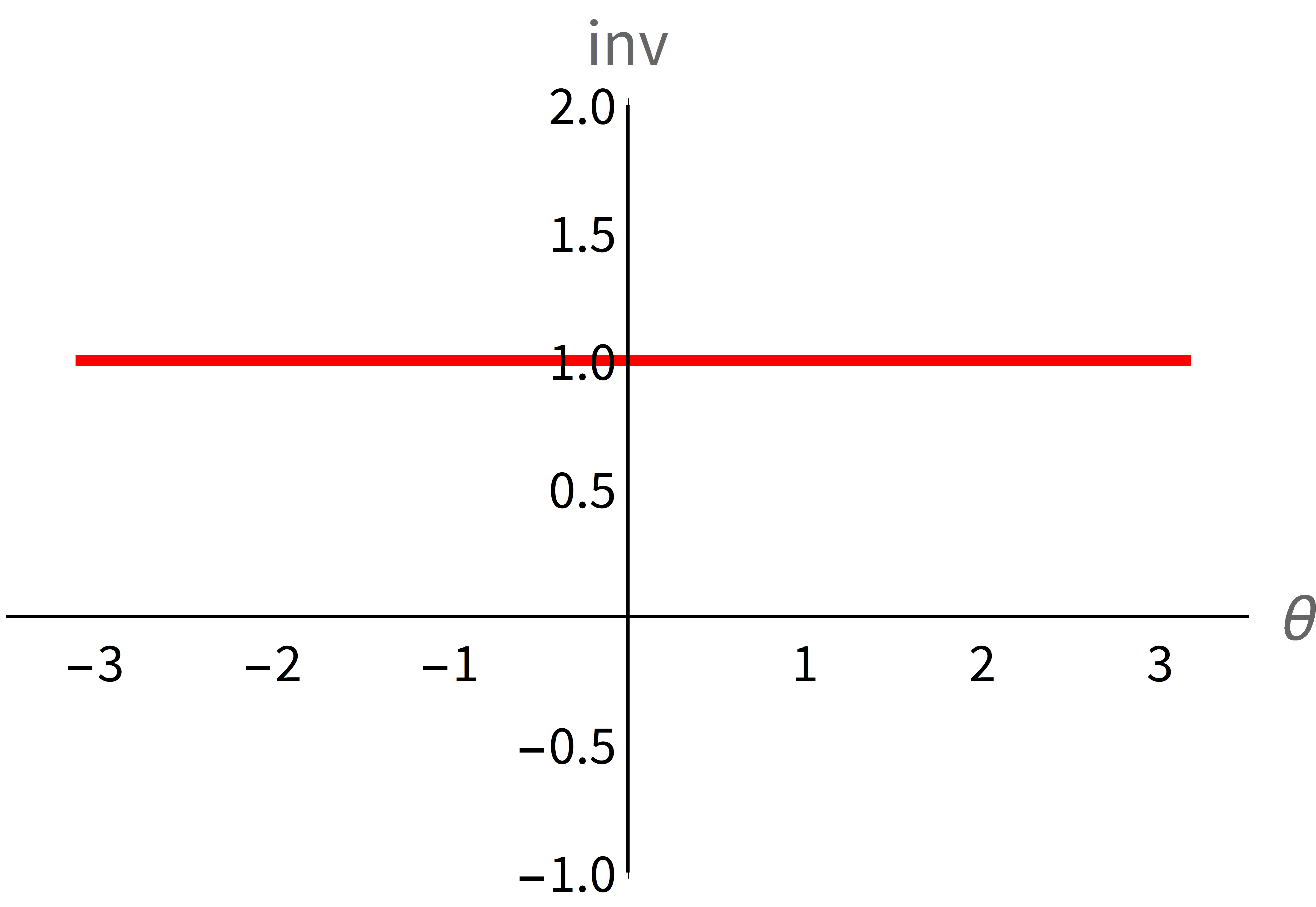
If we take , and , the system is gapped and topological trivial. In this case, for all (Fig.2). For the case , and , this system is gapped and topological non-trivial and for all (Fig.3). For topological non-trivial system, there exist topological state in the spectrum under OBC (Fig.3). For topological trivial system, there exist no topological state in the OBC spectrum (Fig.2). This is consistent with the traditional Hermitian bulk-boundary correspondence.


VI.2 non-Hermitian case
We consider a -dimensional non-Hermitian space-time crystal system with single orbital. For simplicity, we still assume the the lattice potential has the form given by Eqs.(34) and (35) with and . Thus, and for this system, and only , and are nonzero for the tight-binding Hamiltonian given by Eq.(6). Hence, we assume that,
| (50) | |||
| (51) | |||
| (52) |
where is the index of site and is the length of the system. Under PBC, according to Eq.(8) and Appendix A,
| (53) | |||
| (54) | |||
| (55) |
Thus, the effective Hamiltonian under PBC is
| (56) |
where
| (57) | |||
| (58) |
We find that
| (59) |
with , where is the Pauli matrix, is the complete conjugation operator and is the operator acting on creation and annihilation operators,
| (60) |
Thus, this system belongs to class with sublattice symmetry. For given in Eq.(56), the eigenenergy is
| (61) |

For the case , and , for all (Fig.4). According to the definition in Ref.[22], has point gap for all . Thus, this system is gap-preserving if , and . In this case, this system has two topological invariants [22],
| (62) | |||
| (63) |
If , for arbitrary . Thus, this system is gapless in this case.
If we take , and ,
| (64) |
If , for all . If , and . Hence, has point gap and is gapless. This means this system is gap-breaking for the case , and .
VII Conclusion and Discussion
In this work, we show that space-time crystal system can be divided into two classes, rational space-time crystal system and irrational space-time crystal system. A rational space-time crystal system is equal to a traditional floquet system. Then we find a way to solve the floquet equation analytically. Hence, we can obtain the quasi-spectrum and the effective Hamiltonian of the system analytically, and we point out that the physical spectrum of the system is just the th sector of the quasi-spectrum. Then, we discuss the properties of the effective Hamiltonian under internal symmetries and give the types of the Hermitian and non-Hermitian effective Hamiltonian according to the energy gap. There are three types of Hermitian effective Hamiltonian, gapped, half-gapped and gapless. And there are also three types of non-Hermitian effective Hamiltonian, gap-preserving, gap-breaking and gapless. For gapped Hermitian rational space-time crystal systems, the topological classification of them can be reduced to the Hermitian tenfold AZ classes, and for gap-preserving non-Hermitian rational space-time crystal system under PBC, the topological classification of them can be reduced to the non-Hermitian -fold classes with three types of the complex energy gap. Our works give a new perspective of space-time crystal system and pave a way to research rational space-time crystal system systematically.
In the future, the topological classification about the half-gapped and gapless Hermitian rational space-time crystal systems and the topological classification about the gap-breaking and gapless non-Hermitian rational space-time crystal systems will be considered for the complete topological classification of rational space-time crystal systems. Furthermore, the properties of irrational space-time crystal systems will also be discussed in our future work .
VIII acknowledgements
The authors thank useful discussion with Yongxu Fu, Haoshu Li and Zhiwei Yin. This work was supported by NSFC Grant No. 11275180.
Appendix A The Hamiltonian After Taking the New Unit Cell
Consider a site locating at . Under the basis , we can decompose as with . Thus, we can use a column vector to represent ,
| (65) |
The integer can be decomposed to with and . Then, can be rewritten as
| (66) |
After taking as the group of lattice vectors, there are orbitals in a unit cell. In this case, we treat the site locating at under original coordinate as an orbital locating at
| (67) |
with orbital indexes . Then, we define
| (68) |
as the annihilation operator about the new unit cell locating at and are orbital indexes. For
| (69) | |||
| (70) |
we define
| (71) |
For , . Thus, , and
| (72) |
This means the matrix only depends on the value of . Hence, the Hamiltonian in Eq.(6) and Eq.(7) can be written as the Hamiltonian in Eq.(8), which respect the spatial translation symmetry.
Appendix B The Physical Spectrum of The System
For the effective Hamiltonian , we use to represent the eigenvector of with eigenvalue . For a given , are orthogonal and complete,
| (73) |
According to Eq.(10) and Eq.(12), the physical state corresponding to the quasistate is
| (74) |
The expected value of energy about the state under long time average is
| (75) |
According to Eq.(74),
| (76) |
Since
| (77) | |||
| (78) |
Eq.(75) can be reduced as
| (79) |
This means the expected value of energy about the state , which is the physical state corresponding to the quasitate with quasienergy in th sector of the quasi-spectrum, under long time average is still . Hence, the th sector of the quasi-spectrum gives the physical spectrum of the system.
If is non-Hermitian, the eigenvectors of are biorthogonal and complete [20, 21],
| (80) |
where () means this state is a right (left) eigenstate of . In this case,
| (81) | |||
| (82) |
and
| (83) |
Hence, for non-Hermitian rational space-time crystal system, the th sector of the quasi-spectrum still gives the physical spectrum.
Appendix C The Representation of Internal Symmetry on the Effective Hamiltonian
C.1 For Hermitian case
Under PBC, the Hamiltonian in Eq.(8) is written as
| (84) |
Under time-reversal transformation, operator and unit imaginary number are transformed as
| (85) |
where is a unitary matrix. Thus, under TRS, the Hamiltonian is transformed as
| (86) |
where
| (87) |
and means complex conjugation. Thus, the effective Hamiltonian corresponding to is
| (88) |
If the system has TRS, . Hence, for such a system, . Thus,
| (89) |
For PHS,
| (90) |
where, is a unitary matrix. Thus,
| (91) |
where
| (92) |
and we assume that . The effective Hamiltonian corresponding to is
| (93) |
If the system has PHS, . Thus, and
| (94) |
Since CS is the combination of TRS and PHS,
| (95) |
C.2 For Non-Hermitian case
We consider TRS firstly. If a non-Hermitian system has TRS,
| (96) |
with
| (97) |
and is a unitary matrix. TRS in non-Hermitian system has the same form as TRS in Hermitian system. Thus, for non-Hermitian system with TRS,
| (98) |
For non-Hermitian PHS,
| (99) |
with a unitary matrix , and
| (100) |
The form of PHS in Hermitian system and non-Hermitian system are the same. Hence, for non-Hermitian PHS,
| (101) |
Now, we consider TRS† in non-Hermitian system. Under TRS†
| (102) |
with a unitary matrix . However, if a non-Hermitian system has TRS†, the Hamiltonian has the relation
| (103) |
For the Hamiltonian given in Eq.(84) ,
| (104) |
where
| (105) |
Thus, the effective Hamiltonian corresponding to is
| (106) |
According to Eqs.(84),(103) and (104), . Hence,
| (107) |
If a non-Hermitian system has PHS†,
| (108) |
for the Hamiltonian and
| (109) |
with a unitary matrix . For given in Eq.(84),
| (110) |
where
| (111) |
The effective Hamiltonian corresponding to is
| (112) |
Since , . Hence,
| (113) |
Since CS is the combination of TRS and PHS, or the combination of TRS† and PHS†,
| (114) |
SLS is the generalization of CS in non-Hermitian system. For SLS,
| (115) |
where is a unitary matrix with . If satisfies SLS,
| (116) |
According to Eq.(115),
| (117) |
where
| (118) |
Then,
| (119) |
If satisfies Eq.(116), . Hence,
| (120) |
For pseudo-Hermitian symmetry, the operator is a linear operator [29]. Thus,
| (121) |
where is a unitary and Hermitian matrix. If is pseudo-Hermitian,
| (122) |
We know that
| (123) |
where
| (124) |
and the effective Hamiltonian corresponding to is
| (125) |
If satisfies Eq.(122), . Hence,
| (126) |
All above give the effective Hamiltonian transformed under internal symmetries.
Appendix D The Constraints of Space-Time Translation Symmetry Given by TRS
Consider a -dimensional lattice potential with space-time translation symmetry, whose space-time translation vectors are for . That means
| (127) |
for . If is invariant under TRS, we have
| (128) |
where is the time-reversal operator and “” means complex conjugation. Since satisfies Eq.(127) and Eq.(128) simultaneously,
| (129) |
Eq.(129) shows that for a -dimensional space-time crystal system with space-time translation vectors (), if this system is invariant under TRS, () are also space-time translation vectors. Under these constraints, TRS is compatible with space-time translation symmetry.
References
- Chiu et al. [2016] C.-K. Chiu, J. C. Y. Teo, A. P. Schnyder, and S. Ryu, Classification of topological quantum matter with symmetries, Rev. Mod. Phys. 88, 035005 (2016).
- Qi and Zhang [2011] X.-L. Qi and S.-C. Zhang, Topological insulators and superconductors, Rev. Mod. Phys. 83, 1057 (2011).
- Qi et al. [2008] X.-L. Qi, T. L. Hughes, and S.-C. Zhang, Topological field theory of time-reversal invariant insulators, Phys. Rev. B 78, 195424 (2008).
- Tuegel et al. [2019] T. I. Tuegel, V. Chua, and T. L. Hughes, Embedded topological insulators, Phys. Rev. B 100, 115126 (2019).
- Po et al. [2018] H. C. Po, H. Watanabe, and A. Vishwanath, Fragile topology and wannier obstructions, Phys. Rev. Lett. 121, 126402 (2018).
- Alexandradinata et al. [2011] A. Alexandradinata, T. L. Hughes, and B. A. Bernevig, Trace index and spectral flow in the entanglement spectrum of topological insulators, Phys. Rev. B 84, 195103 (2011).
- Benalcazar et al. [2017] W. A. Benalcazar, B. A. Bernevig, and T. L. Hughes, Electric multipole moments, topological multipole moment pumping, and chiral hinge states in crystalline insulators, Phys. Rev. B 96, 245115 (2017).
- Benalcazar et al. [2019] W. A. Benalcazar, T. Li, and T. L. Hughes, Quantization of fractional corner charge in -symmetric higher-order topological crystalline insulators, Phys. Rev. B 99, 245151 (2019).
- Liu et al. [2019] T. Liu, Y.-R. Zhang, Q. Ai, Z. Gong, K. Kawabata, M. Ueda, and F. Nori, Second-order topological phases in non-hermitian systems, Phys. Rev. Lett. 122, 076801 (2019).
- Kawabata et al. [2021] K. Kawabata, K. Shiozaki, and S. Ryu, Topological field theory of non-hermitian systems, Phys. Rev. Lett. 126, 216405 (2021).
- Fu et al. [2021] Y. Fu, J. Hu, and S. Wan, Non-hermitian second-order skin and topological modes, Phys. Rev. B 103, 045420 (2021).
- Okuma et al. [2020] N. Okuma, K. Kawabata, K. Shiozaki, and M. Sato, Topological origin of non-hermitian skin effects, Phys. Rev. Lett. 124, 086801 (2020).
- Li and Wan [2021] H. Li and S. Wan, Homotopy invariant in time-reversal and twofold rotation symmetric systems, Phys. Rev. B 104, 045150 (2021).
- Roy and Harper [2017] R. Roy and F. Harper, Periodic table for floquet topological insulators, Phys. Rev. B 96, 155118 (2017).
- Fu and Kane [2006] L. Fu and C. L. Kane, Time reversal polarization and a adiabatic spin pump, Phys. Rev. B 74, 195312 (2006).
- Fu and Kane [2007] L. Fu and C. L. Kane, Topological insulators with inversion symmetry, Phys. Rev. B 76, 045302 (2007).
- Borgnia et al. [2020] D. S. Borgnia, A. J. Kruchkov, and R.-J. Slager, Non-hermitian boundary modes and topology, Phys. Rev. Lett. 124, 056802 (2020).
- Wu and An [2020] H. Wu and J.-H. An, Floquet topological phases of non-hermitian systems, Phys. Rev. B 102, 041119 (2020).
- Yao et al. [2017] S. Yao, Z. Yan, and Z. Wang, Topological invariants of floquet systems: General formulation, special properties, and floquet topological defects, Phys. Rev. B 96, 195303 (2017).
- Shen et al. [2018] H. Shen, B. Zhen, and L. Fu, Topological band theory for non-hermitian hamiltonians, Phys. Rev. Lett. 120, 146402 (2018).
- Yao et al. [2018] S. Yao, F. Song, and Z. Wang, Non-hermitian chern bands, Phys. Rev. Lett. 121, 136802 (2018).
- Kawabata et al. [2019] K. Kawabata, K. Shiozaki, M. Ueda, and M. Sato, Symmetry and topology in non-hermitian physics, Phys. Rev. X 9, 041015 (2019).
- Xu and Wu [2018] S. Xu and C. Wu, Space-time crystal and space-time group, Phys. Rev. Lett. 120, 096401 (2018).
- Peng [2022] Y. Peng, Topological space-time crystal, Phys. Rev. Lett. 128, 186802 (2022).
- Note [1] At least one number of is nonzero.
- Note [2] We take as the space-time metric to make it consistent with Refs.[23],[24].
- Sambe [1973] H. Sambe, Steady states and quasienergies of a quantum-mechanical system in an oscillating field, Phys. Rev. A 7, 2203 (1973).
- Chen et al. [2018] Q. Chen, L. Du, and G. A. Fiete, Floquet band structure of a semi-dirac system, Phys. Rev. B 97, 035422 (2018).
- Mostafazadeh [2002] A. Mostafazadeh, Pseudo-hermiticity versus pt-symmetry iii: Equivalence of pseudo-hermiticity and the presence of antilinear symmetries, Journal of Mathematical Physics 43, 3944 (2002), https://doi.org/10.1063/1.1489072 .