Topological charge pumping in excitonic insulators
Abstract
We show that in excitonic insulators with -wave electron-hole pairing, an applied electric field (either pulsed or static) can induce a -wave component to the order parameter, and further drive it to rotate in the plane, realizing a Thouless charge pump. In one dimension, each cycle of rotation pumps exactly two electrons across the sample. Higher dimensional systems can be viewed as a stack of one dimensional chains in momentum space in which each chain crossing the fermi surface contributes a channel of charge pumping. Physics beyond the adiabatic limit, including in particular dissipative effects is discussed.
Controlling many-body systems, and in particular using appropriately applied external fields to ‘steer’ order parameters of symmetry broken phases, has emerged as a central theme in current physics Kirilyuk et al. (2010); Mentink et al. (2015); Byrnes et al. (2014); Zhang and Averitt (2014); Basov et al. (2017); Golež et al. (2016); Claassen et al. (2019); Sun and Millis (2020a). The excitonic insulator (EI) is state of matter first proposed in the 1960s Mott (1961); Kozlov and Maksimov (1965); Jérome et al. (1967); Portengen et al. (1996) with an order parameter defined as a condensate of bound electron hole pairs that activates a hybridization between two otherwise (in the simplest case) decoupled bands and opens a gap in the electronic spectrum. Several candidate materials including electron-hole bilayers Fogler et al. (2014); Li et al. (2017); Du et al. (2017), Ta2NiSe5 Lu et al. (2017); Werdehausen et al. (2018); Wakisaka et al. (2009); Kaneko et al. (2013); Sugimoto et al. (2018); Mazza et al. (2020), -TiSe2 Kogar et al. (2017); Cercellier et al. (2007); Kaneko et al. (2018); Chen et al. (2018) and monolayer WTe2 Jia et al. (2020) are objects of current intensive study; recent work Du et al. (2017); Hu et al. (2018); Wang et al. (2019); Hu et al. (2020); Varsano et al. (2020); Perfetto and Stefanucci (2020); Hou et al. (2019) has pointed out their possible topological aspects. While the early theories of EI considered a one component order parameter, typically of inversion symmetric -wave type, realistic interactions also allow for electron-hole pairing in sub-dominant channels including -wave (inversion-odd) ones. In equilibrium, the -wave ground state is favored, with the potential for -wave order revealed by its fluctuations accompanied by dipole moment oscillations: the ‘Bardasis-Schrieffer’ collective mode Sun and Millis (2020b).
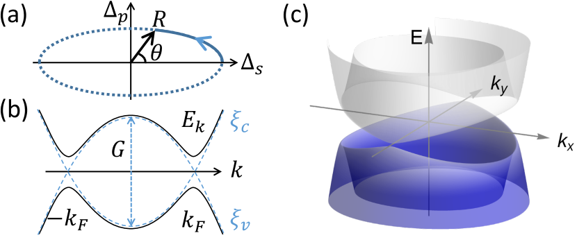
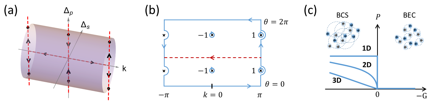
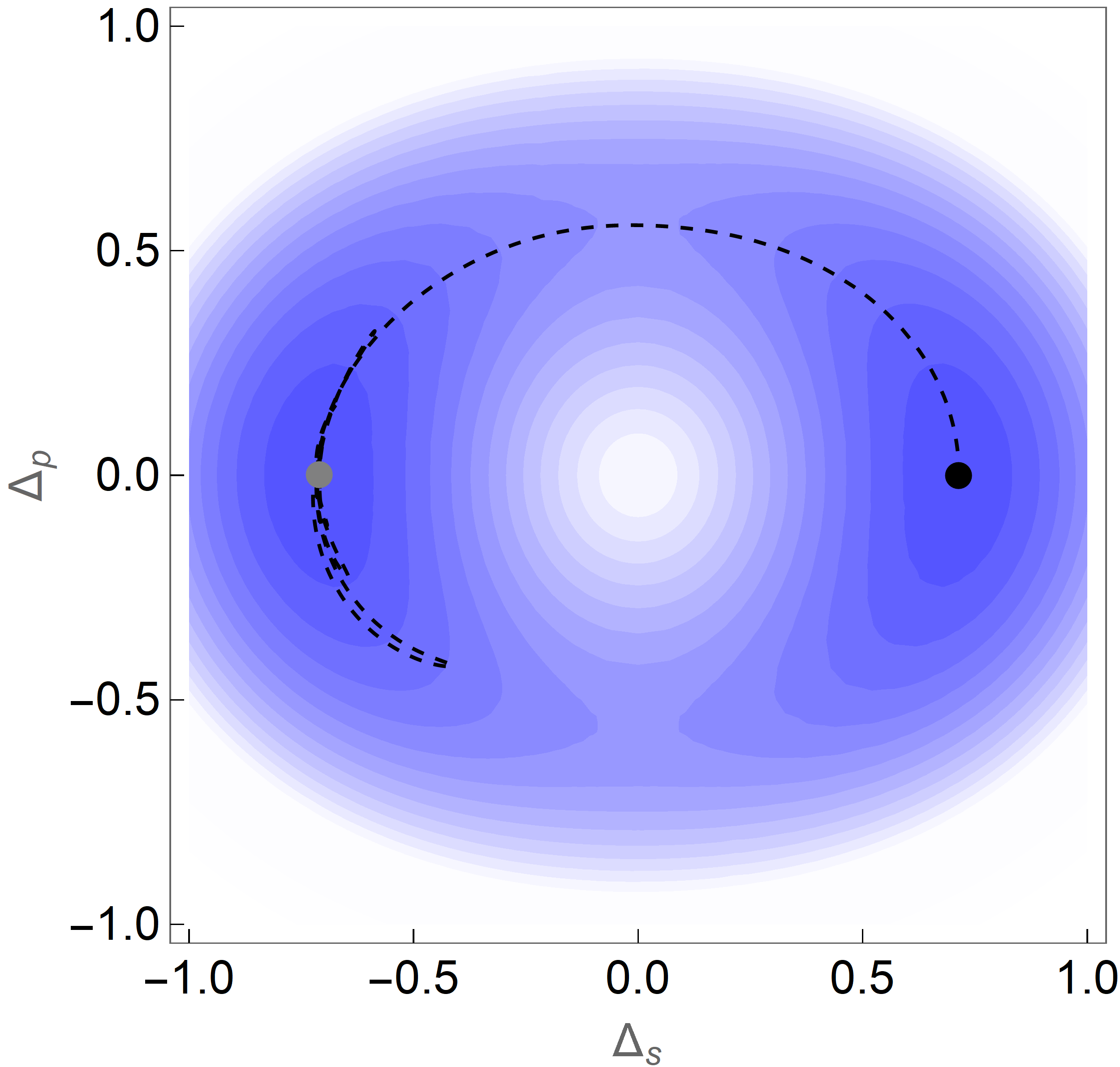
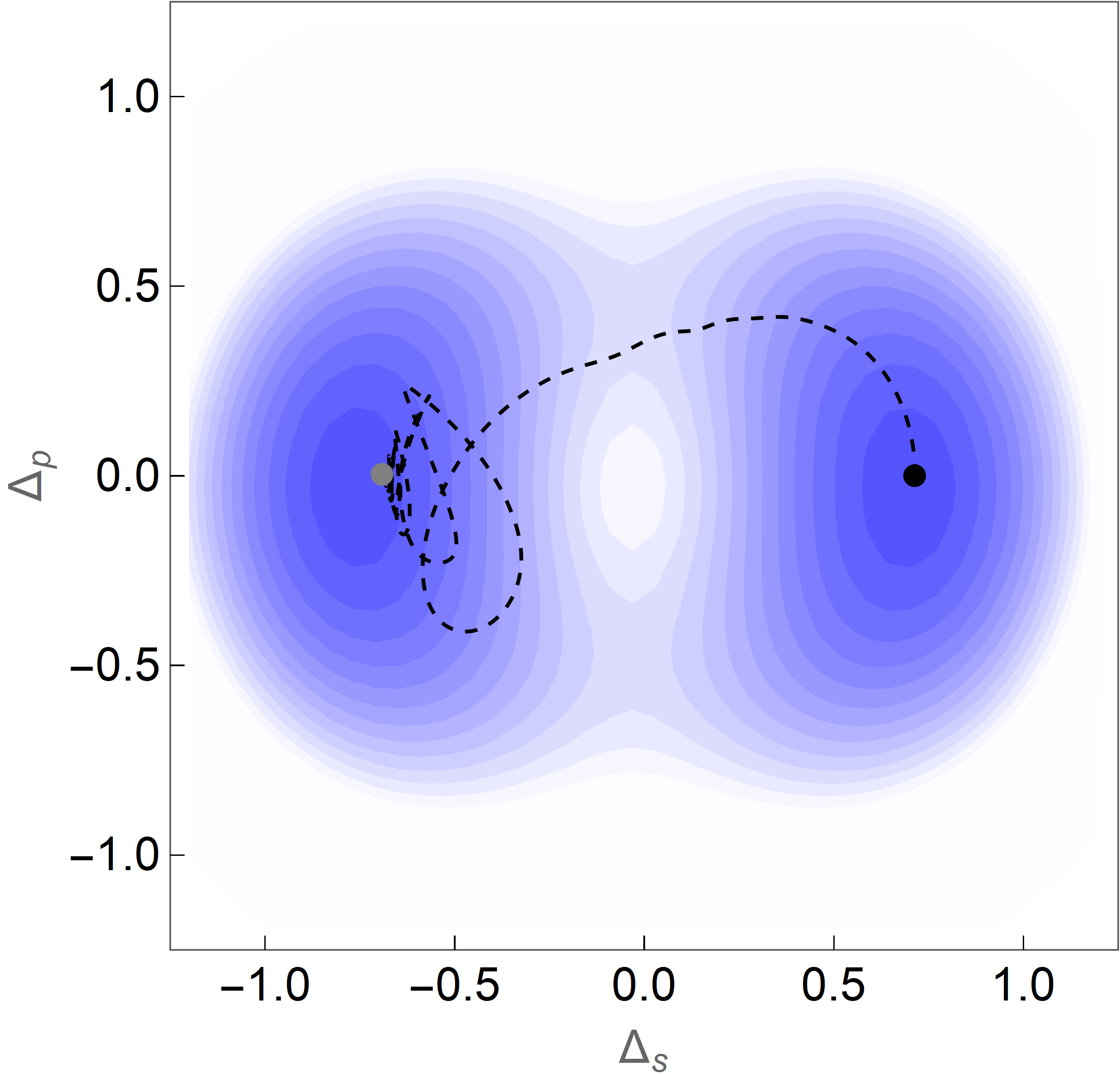
In this paper we show that applied electric fields can steer the order parameter to rotate in the space of s and p symmetry components, as shown in Fig. 1(a), leading to a realization of the ‘Thouless charge pump’ Thouless (1983); Rice and Mele (1982); King-Smith and Vanderbilt (1993); Zhang et al. (2020), providing quantized charge transport across an insulating sample.
The minimal model of an EI involves two electron bands shown in Fig. 1(b): a valence band with energy that disperses downwards from a high symmetry point (taken to have zero momentum) and a conduction band () that disperses upwards. For simplicity we assume that their energies are equal and opposite (). Relaxing this assumption does not change our results in an essential way. Defining the overlap , we distinguish the ‘BCS’ case where the two bands cross at a fermi wavevector with fermi velocity as shown by the dashed lines, leading to electron and hole pockets, and the ‘BEC’ case where and the bands do not cross. Excitonic order corresponds to the spontaneous formation of a hybridization between the two bands due to the electron-electron interaction , leading to an order parameter where is the electron annihilation operator at momentum of the conduction/valence band and is the Fourier transform of the density-density interaction potential . The -wave order parameter is invariant under crystal symmetry operations while -wave order parameters are odd under inversion: , and often transform as a multi-dimensional representation of the crystal symmetry group. For simplicity we neglect the -dependence of , and define where the pairing function carries the momentum dependence and satisfies . We focus on the pairing channel which is induced by the x-direction electric fields we consider here. While the qualitative conclusions hold generically for all spatial dimensions, we will indicate the dimensionality if a specific d-dimensional system is discussed where the momentum means a d-dimensional vector.
Writing the partition function as a path integral over fermion fields , performing a Hubbard-Stratonovich transformation of the interaction term in the excitonic pairing channel and subsuming the intraband interaction into one obtains the action (see SI Sec. I)
| (1) |
as an integral over space-time and the partition function is . For physically reasonable interactions such as the screened Coulomb interaction, the -wave pairing interaction is typically the strongest while is the leading subdominant one. We may write the mean field Hamiltonian as with
| (2) |
where are the Pauli matrices acting in the c/v band space. The vector potential enters Eq. (2) through the minimal coupling required by local gauge invariance (electric field is ) and we set electron charge , speed of light and the Planck constant to be one. Interband dipolar couplings could also occur Golež et al. (2016); Murakami et al. (2020) but do not affect our results. Since the global phase is not important, we choose the -wave order parameter to be real. As we will show, the system develops an electrical polarization as a -wave component out of phase with the equilibrium is introduced. Due to an emergent ‘particle hole’ symmetry in the BCS weak coupling case defined as which we focus on, applied electric fields create primarily in this channel (see Sec. VI A of SI for a rigorous proof), so we write -wave pairing in the channel Sun and Millis (2020b). The quasiparticle spectrum is . As shown by Fig. 1(c), the spectrum will have gapless points (nodes) at in the pure -wave state () in two dimensions (2D).
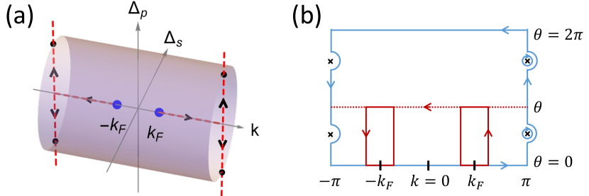
Charge pump—Spatially uniform changes in produce uniform currents (see SI Sec. II), whose time integral from the initial to the final point then gives the pumped charge (difference of polarization between the final state and the initial state). In a one dimensional (1D) system, has a geometrical meaning King-Smith and Vanderbilt (1993); Resta (1994) in the limit of slow order parameter dynamics. It is the flux of the Berry curvature 2-form through the 2D surface spanned by the occupied 1D crystal momentum and the time varying trajectory of , or alternatively by the line integral of the Berry connection around its boundary:
| (3) |
where (see Fig. 2).
The Berry curvature from the valence band of Eq. (2) is sourced by monopoles at the points , i.e., the points each of which has monopole charge . If the order parameter evolution completes a full cycle on the plane, becomes the surface of the 2-torus shown in Fig. 2(a) and the net charge pumped is the total flux from the enclosed monopoles which is an integer , the Chern number of the process. This quantized change in the polarization is known as the Thouless pump Thouless (1983), a topological phenomenon immune to disorder. Note that the monopoles exist only for the ‘BCS’ (, band inversion) case where the excitons strongly overlap such that charge can jump between them. In the ‘BEC’ case for all and there are no monopoles enclosed in (see SI Sec. II C).
To compute the polarization for the case the order parameter does not complete a full cycle, we use the line integral approach. For notational simplicity, we suppress the subscripts ‘’ without causing ambiguities. An explicit expression for the valence band wave function from (2) at is
| (4) |
where and . The Berry connection has singularities associated with the Dirac strings, the intersections of which with (marked by crosses in Fig. 2(b)) must be correctly treated in the evaluation of the line integral. Noting that when and when , we see that in the weak coupling BCS limit the contour can be collapsed to the red rectangles in Fig. 2(b). Parameterizing using and the angle defined by in Fig. 1(a), one observes that the polarization of an state on the plane depends only on the angle . Specifically, we found
| (5) |
for a 1D EI (see SI Sec. II). This may be understood by noting that the low energy physics around is of two massive Dirac models, each of which realizes a Goldstone-Wilczek Goldstone and Wilczek (1981) mechanism of charge pumping.
Higher dimensional systems can be viewed as 1D chains along direction stacked in momentum space. For a 2D circular fermi surface one finds
| (9) |
A full cycle pumps exactly two electrons along each 1D momentum chain that crosses the fermi surface, giving
| (10) |
for 1D, 2D and three dimensional (3D) isotropic systems respectively.
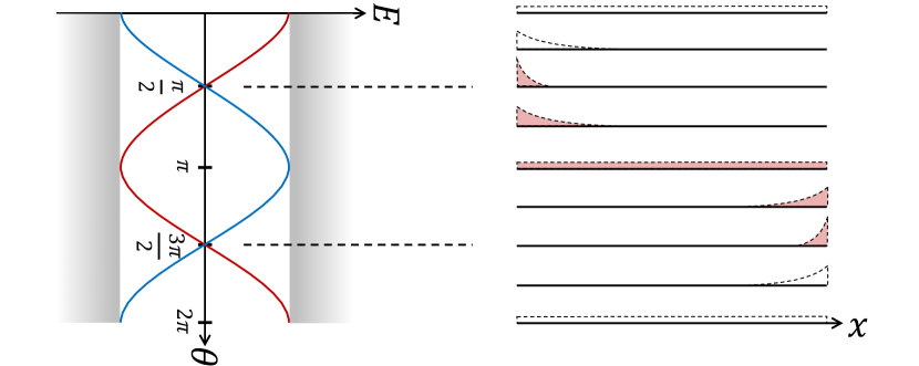
Although the charge pump is a bulk property carried by all valence band electrons, it is also revealed by the evolution of edge states Yang et al. (2020) as and are varied, as shown in Fig. 3 for a 1D wire connected with reservoirs. In the BCS limit, with open boundary conditions , there are two edge states
| (11) |
where is a normalization constant. We suppose and follow the evolution of as is varied (see Fig.3). At the state is delocalized and unoccupied with energy . As is increased the state becomes localized near and decreases in energy. When passes through , the state becomes maximally localized and becomes occupied by an electron from the left reservoir since its energy crosses the chemical potential. As further increases the state becomes delocalized and then localized at the right edge, delivering its electron to the right reservoir when crosses . Considering the state during the same cycle, two electrons in total are pumped. In higher dimensions, each 1D chain crossing the fermi surface has a similar edge state evolution (see SI Sec. III).
Dynamics—The coupled dynamics of electrons and the order parameters in the presence of an applied electric field is described by the action Eq. (1). To understand the qualitative dynamics, we use a low energy effective Ginzburg-Landau Lagrangian
| (12) |
for fields obtained by integrating out the Fermions (see SI Sec. IV). The dynamics is given by the standard Euler-Lagrange equation and is that of a point particle moving in the landscape defined by , with kinetic energy and driven by an electric field through . We find
| (13) |
where is the adiabatic polarization in Eqs. (5) or (9), and is the optical conductivity from virtual interband excitations (see SI Sec. IV). It is natural that electric field couples linearly to the polarization and therefore provides a ‘force’ to rotate the order parameter in the plane.
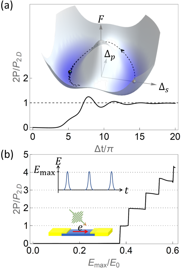
gives the potential landscape in which the dynamics takes place; it has the anisotropic ‘Mexican hat’ form shown in Fig. 4(a). For (quasi) 1D systems in the weak coupling BCS limit Altland and Simons (2010); Sun et al. (2020):
| (14) |
where is density of states in the metallic phase and is a high energy cutoff Kozlov and Maksimov (1965). The first term becomes for a 2D isotropic Fermi surface and for 3D where and are angular variables on the Fermi surface. The landscape has a local maximum at surrounded by a trough at of lower values of . The ground state minima are at and the pure p-wave phases at are saddle points with energy higher by where is a constant depending on the space dimension.
We may estimate the minimal electric field required to drive the system from the minimum through the -wave saddle point by equating the potential energy barrier to the work done by the electric field, obtaining
| (15) |
where is the coherence length (exciton size), in 1D and in 2D, and is at the order of the dielectric breakdown field. For , and , such as the case of electron hole bilayers, the threshold field is which can be easily achieved by modern optical technique. For a gap such as that in Ta2NiSe5 Lu et al. (2017); Werdehausen et al. (2018) (assuming it is in the BCS regime), the threshold field is about . At such large field, terms in the Lagrangian will be important, which pushes the order parameter closer to zero but does not destroy the qualitative dynamics in the transient regime (See SI Sec. IV D).
The dynamical term has a relatively simple form if the gap never closes on the Fermi surface and the order parameter variation timescale is long compared to the inverse of the gap. For example for (quasi) 1D
| (16) |
to lowest order in time derivatives. For higher dimensions with closed Fermi surfaces, there are changes to the coefficients and, crucially, dissipation and time non-locality arises from quasiparticle excitations near the nodes of the p-wave gap when passes zero. This dissipation also brings a correction to the pumped charge: . To estimate , we observe that as the order parameter passes this gapless regime with a velocity , the probability for exciting a particle-hole pair at is given by the Landau-Zener formula Wittig (2005): where is half of its minimal excitation energy during the dynamics. In 2D, summing over momenta, one obtains the number of excited quasi particles and the non-adiabatic correction to the pumped charge
| (17) |
valid if (see SI Sec. VI C). Therefore, if the sub-dominant -wave coupling constant is too small such that , this dissipative correction will dominate over the adiabatic charge.
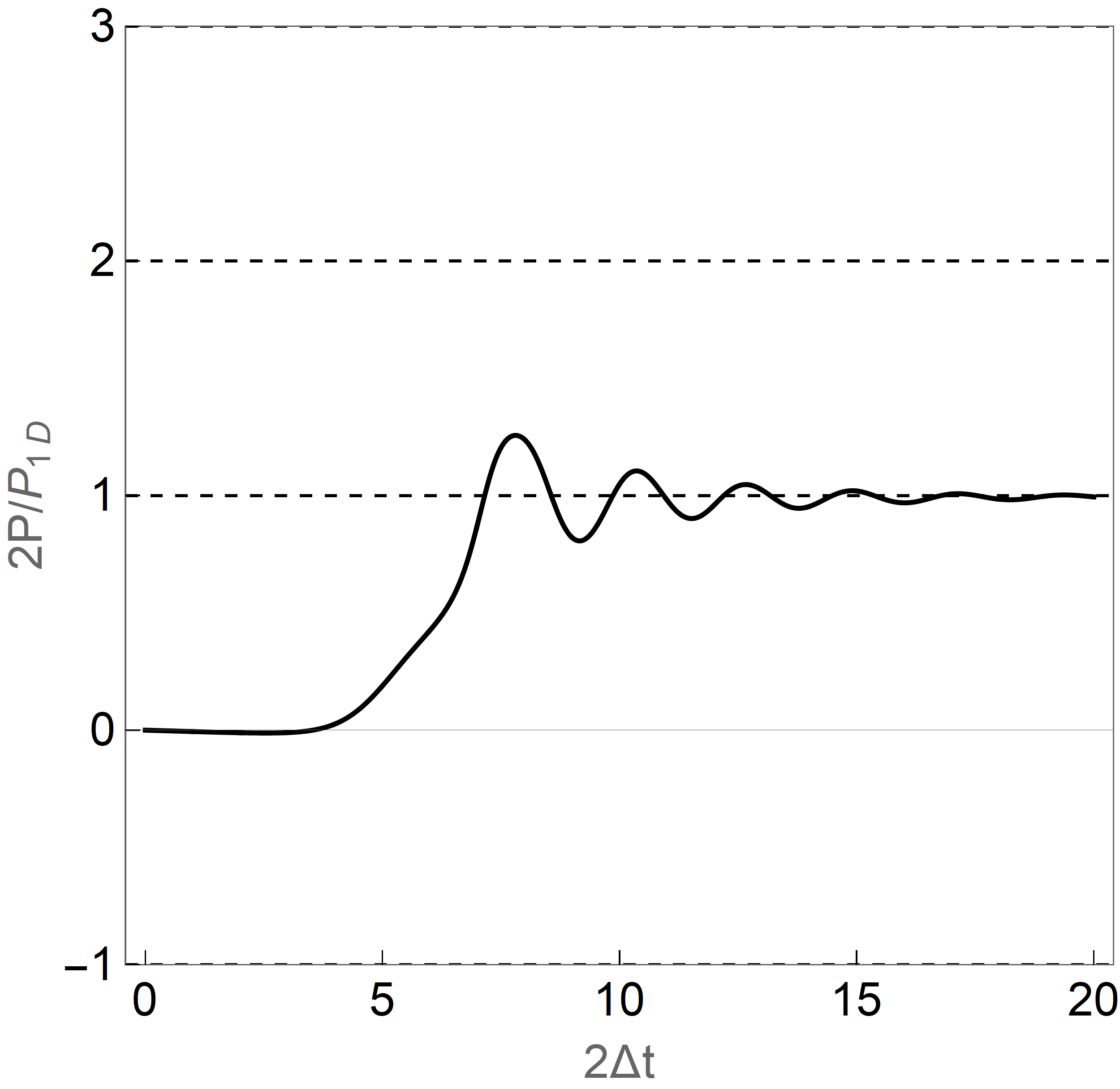
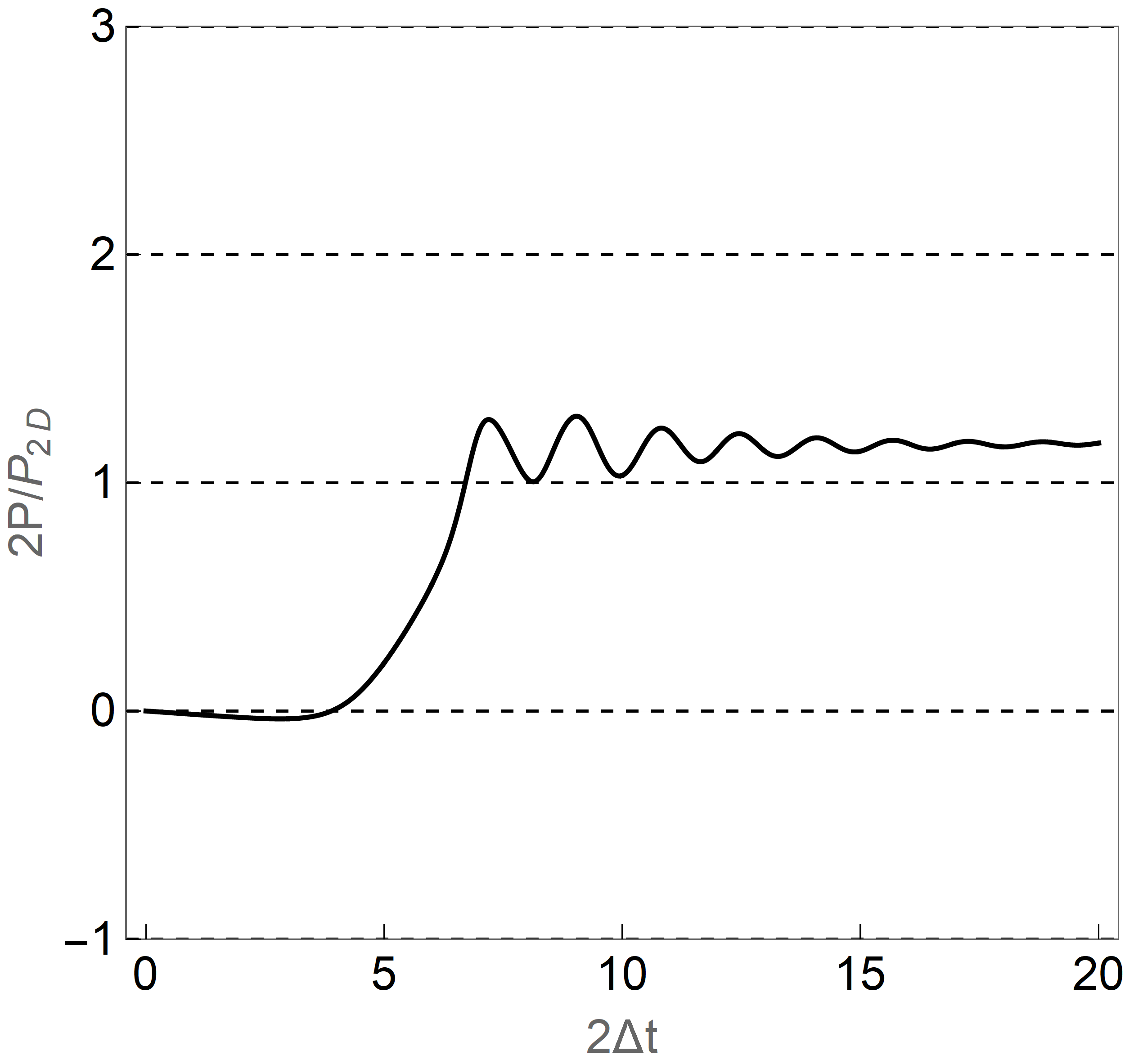
Numerics and Experiment—We numerically solved the mean field dynamics implied by Eq. (1) for a BCS weak coupling EI in 2D, driven by a train of widely separated electric field pulses (Fig. 4(b)). Mean field dynamics Barankov et al. (2004) means that each momentum state evolves in the time dependent mean field with determined self consistently by the gap equation, neglecting any spatial fluctuations. We include a weak phenomenological damping to represent energy loss caused by, e.g., a phonon bath (see SI Sec. VI). Each pulse drives the order parameter along the trajectory shown as the black dashed line in Fig. 4(a), advancing it by to stabilize the system in the other -wave ground state. The total duration of the evolution from one minimum to the next is and the amount of charge pumped is where is the width of the sample, as shown by Fig. 4(a). In a train of pulses with inter pulse separation , each pulse advances the order parameter from one minimum to the next and allows it to stabilize before next pulse arrives, leading to a time-averaged current . For a wide sample with normal state carrier density of and inter pulse time , the current is considering spin degeneracy.
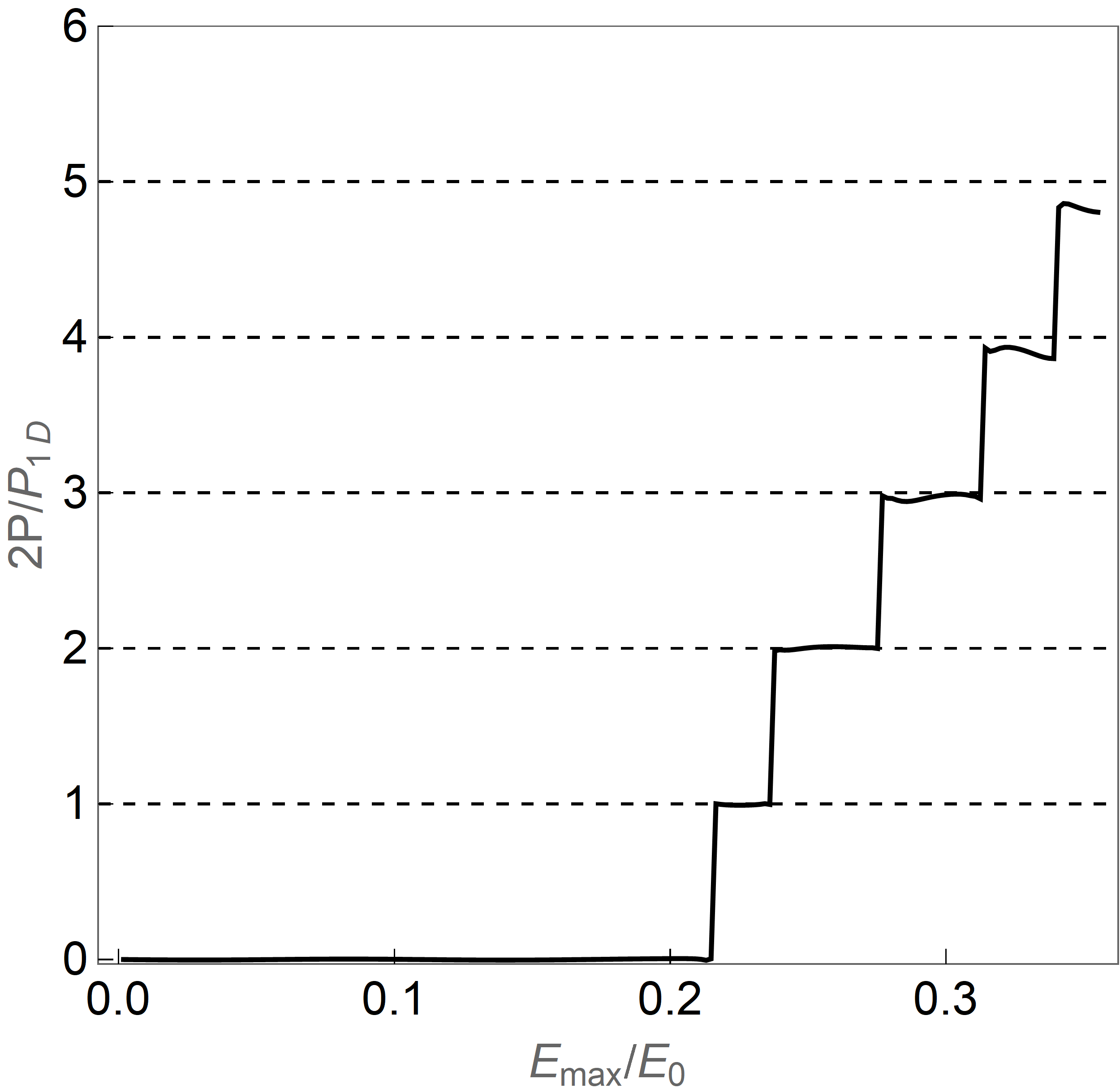
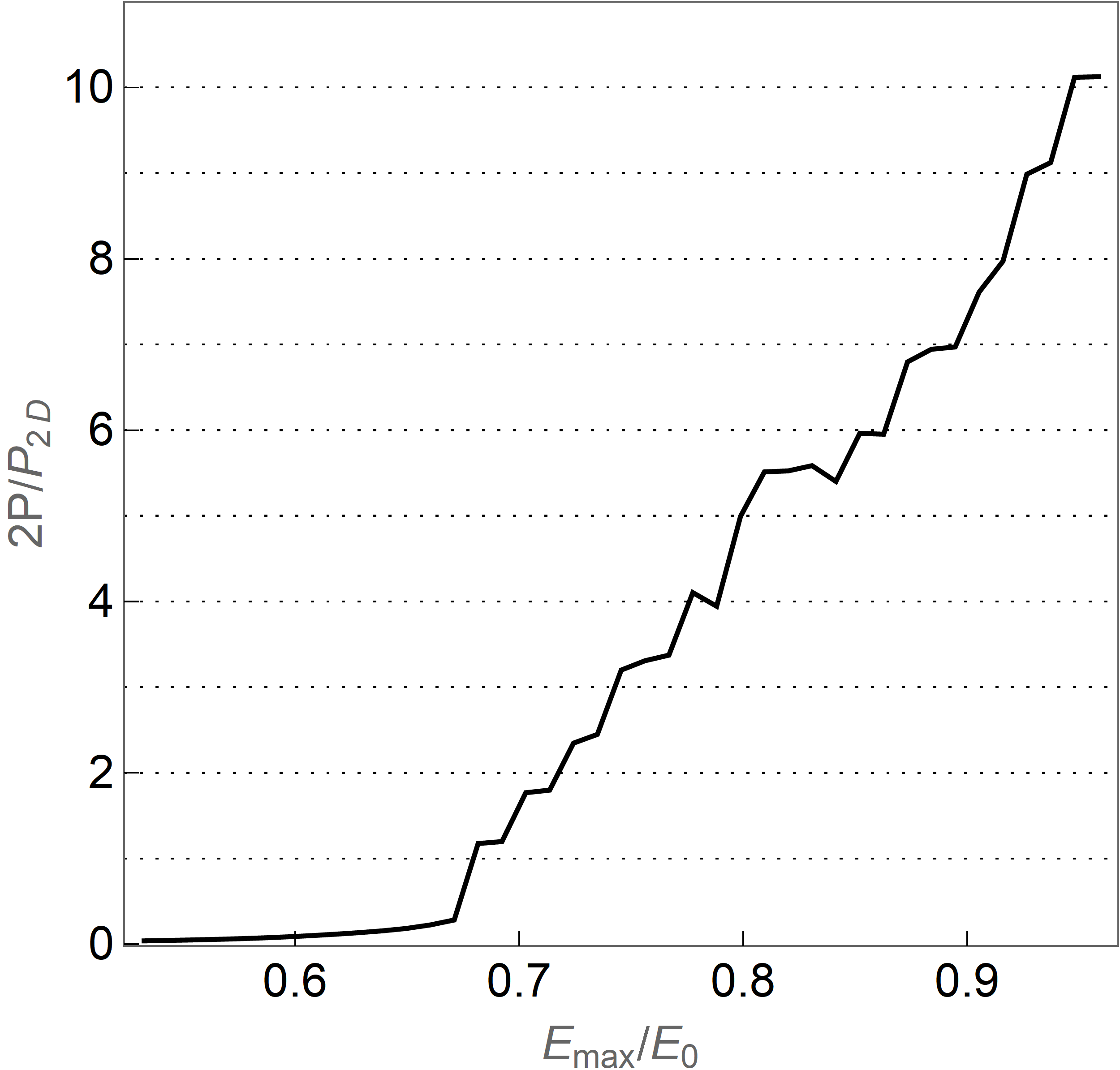
A minimum field strength (15) is required: as the maximum electric field of the pulse is increased beyond the threshold, the charge pumping (DC current) will onset sharply, as shown in Fig. 4(b). As further increases, each pulse induces a rotation of more cycles which pumps more charge, giving rise to the step structure. Deviations from perfect quantization arise from fast order parameter dynamics caused by the short duration pulse. A precisely engineered long duration pulse can substantially reduce these deviations; see SI Sec. V.
A static electric field in the DC transport regime could also drive such an order parameter rotation and charge pumping. However, unlike the case of well separated pulses, there is no time break to dump the generated heat into the environment which might destroy the system.
Discussion—We have shown theoretically that a Thouless charge pump may be realized as a collective many-body effect arising from order parameter steering in BCS type excitonic insulators. Similar dynamics and charge pumping can occur in general when the ground state order parameter and the sub dominant one have different parities under inversion. Its observation would provide both a verification of order parameter steering and a probe of the excitonic insulating state, in particular, distinguishing BCS and BEC states. It is interesting to study the dynamics in the vicinity of the BCS-BEC crossover and effects beyond mean field.
Acknowledgements.
We acknowledge support from the Energy Frontier Research Center on Programmable Quantum Materials funded by the US Department of Energy (DOE), Office of Science, Basic Energy Sciences (BES), under award No. DE-SC0019443. We thank W. Yang, D. Golez and T. Kaneko for helpful discussions.References
- Kirilyuk et al. (2010) A. Kirilyuk, A. V. Kimel, and T. Rasing, Rev. Mod. Phys. 82, 2731 (2010).
- Mentink et al. (2015) J. H. Mentink, K. Balzer, and M. Eckstein, Nature Communications 6, 6708 (2015).
- Byrnes et al. (2014) T. Byrnes, N. Y. Kim, and Y. Yamamoto, Nature Physics 10, 803 (2014).
- Zhang and Averitt (2014) J. Zhang and R. Averitt, Annu. Rev. Mater. Res. 44, 19 (2014).
- Basov et al. (2017) D. N. Basov, R. D. Averitt, and D. Hsieh, Nature Materials 16, 1077 (2017).
- Golež et al. (2016) D. Golež, P. Werner, and M. Eckstein, Phys. Rev. B 94, 035121 (2016).
- Claassen et al. (2019) M. Claassen, D. M. Kennes, M. Zingl, M. A. Sentef, and A. Rubio, Nature Physics 15, 766 (2019).
- Sun and Millis (2020a) Z. Sun and A. J. Millis, Phys. Rev. X 10, 021028 (2020a).
- Mott (1961) N. F. Mott, Philos. Mag. 6, 287 (1961).
- Kozlov and Maksimov (1965) A. Kozlov and L. Maksimov, Sov. J. Exp. Theor. Phys. 21, 790 (1965).
- Jérome et al. (1967) D. Jérome, T. M. Rice, and W. Kohn, Phys. Rev. 158, 462 (1967).
- Portengen et al. (1996) T. Portengen, T. Östreich, and L. J. Sham, Phys. Rev. B 54, 17452 (1996).
- Fogler et al. (2014) M. M. Fogler, L. V. Butov, and K. S. Novoselov, Nat. Commun. 5, 4555 (2014).
- Li et al. (2017) J. I. A. Li, T. Taniguchi, K. Watanabe, J. Hone, and C. R. Dean, Nature Physics 13, 751 (2017).
- Du et al. (2017) L. Du, X. Li, W. Lou, G. Sullivan, K. Chang, J. Kono, and R.-R. Du, Nature Communications 8, 1971 (2017).
- Lu et al. (2017) Y. F. Lu, H. Kono, T. I. Larkin, A. W. Rost, T. Takayama, A. V. Boris, B. Keimer, and H. Takagi, Nat. Commun. 8, 1 (2017).
- Werdehausen et al. (2018) D. Werdehausen, T. Takayama, M. Höppner, G. Albrecht, A. W. Rost, Y. Lu, D. Manske, H. Takagi, and S. Kaiser, Science Advances 4, eaap8652 (2018).
- Wakisaka et al. (2009) Y. Wakisaka, T. Sudayama, K. Takubo, T. Mizokawa, M. Arita, H. Namatame, M. Taniguchi, N. Katayama, M. Nohara, and H. Takagi, Phys. Rev. Lett. 103, 026402 (2009).
- Kaneko et al. (2013) T. Kaneko, T. Toriyama, T. Konishi, and Y. Ohta, Phys. Rev. B 87, 035121 (2013).
- Sugimoto et al. (2018) K. Sugimoto, S. Nishimoto, T. Kaneko, and Y. Ohta, Phys. Rev. Lett. 120, 247602 (2018).
- Mazza et al. (2020) G. Mazza, M. Rösner, L. Windgätter, S. Latini, H. Hübener, A. J. Millis, A. Rubio, and A. Georges, Phys. Rev. Lett. 124, 197601 (2020).
- Kogar et al. (2017) A. Kogar, M. S. Rak, S. Vig, A. A. Husain, F. Flicker, Y. I. Joe, L. Venema, G. J. MacDougall, T. C. Chiang, E. Fradkin, J. Van Wezel, and P. Abbamonte, Science 358, 1314 (2017).
- Cercellier et al. (2007) H. Cercellier, C. Monney, F. Clerc, C. Battaglia, L. Despont, M. G. Garnier, H. Beck, P. Aebi, L. Patthey, H. Berger, and L. Forró, Phys. Rev. Lett. 99, 146403 (2007).
- Kaneko et al. (2018) T. Kaneko, Y. Ohta, and S. Yunoki, Phys. Rev. B 97, 155131 (2018).
- Chen et al. (2018) C. Chen, B. Singh, H. Lin, and V. M. Pereira, Phys. Rev. Lett. 121, 226602 (2018).
- Jia et al. (2020) Y. Jia, P. Wang, C.-L. Chiu, Z. Song, G. Yu, B. J., S. Lei, S. Klemenz, F. A. Cevallos, M. Onyszczak, N. Fishchenko, X. Liu, G. Farahi, F. Xie, Y. Xu, K. Watanabe, T. Taniguchi, B. A. Bernevig, R. J. Cava, L. M. Schoop, A. Yazdani, and S. Wu, “Evidence for a monolayer excitonic insulator,” (2020), arXiv:2010.05390 [cond-mat.mes-hall] .
- Hu et al. (2018) Y. Hu, J. W. F. Venderbos, and C. L. Kane, Phys. Rev. Lett. 121, 126601 (2018).
- Wang et al. (2019) R. Wang, O. Erten, B. Wang, and D. Y. Xing, Nat. Commun. 10, 1 (2019).
- Hu et al. (2020) L.-H. Hu, R.-X. Zhang, F.-C. Zhang, and C. Wu, Phys. Rev. B 102, 235115 (2020).
- Varsano et al. (2020) D. Varsano, M. Palummo, E. Molinari, and M. Rontani, Nature Nanotechnology 15, 367 (2020).
- Perfetto and Stefanucci (2020) E. Perfetto and G. Stefanucci, Phys. Rev. Lett. 125, 106401 (2020).
- Hou et al. (2019) Y. Hou, R. Wang, R. Xiao, L. McClintock, H. Clark Travaglini, J. Paulus Francia, H. Fetsch, O. Erten, S. Y. Savrasov, B. Wang, A. Rossi, I. Vishik, E. Rotenberg, and D. Yu, Nature Communications 10, 5723 (2019).
- Sun and Millis (2020b) Z. Sun and A. J. Millis, Phys. Rev. B 102, 041110(R) (2020b).
- Thouless (1983) D. J. Thouless, Phys. Rev. B 27, 6083 (1983).
- Rice and Mele (1982) M. J. Rice and E. J. Mele, Phys. Rev. Lett. 49, 1455 (1982).
- King-Smith and Vanderbilt (1993) R. D. King-Smith and D. Vanderbilt, Phys. Rev. B 47, 1651(R) (1993).
- Zhang et al. (2020) Y. Zhang, Y. Gao, and D. Xiao, Phys. Rev. B 101, 041410(R) (2020).
- (38) See Supplemental Material for details of derivation.
- Murakami et al. (2020) Y. Murakami, D. Golež, T. Kaneko, A. Koga, A. J. Millis, and P. Werner, Phys. Rev. B 101, 195118 (2020).
- Resta (1994) R. Resta, Rev. Mod. Phys. 66, 899 (1994).
- Goldstone and Wilczek (1981) J. Goldstone and F. Wilczek, Phys. Rev. Lett. 47, 986 (1981).
- Yang et al. (2020) W. Yang, C. Xu, and C. Wu, Phys. Rev. Research 2, 042047 (2020).
- Altland and Simons (2010) A. Altland and B. D. Simons, Condensed Matter Field Theory (Cambridge University Press, Cambridge, 2010).
- Sun et al. (2020) Z. Sun, M. M. Fogler, D. N. Basov, and A. J. Millis, Phys. Rev. Research 2, 023413 (2020).
- Wittig (2005) C. Wittig, J. Phys. Chem. B 109, 8428 (2005).
- Barankov et al. (2004) R. A. Barankov, L. S. Levitov, and B. Z. Spivak, Phys. Rev. Lett. 93, 160401 (2004).
Supplemental Material for ‘Topological charge pumping in excitonic insulators’
I The Hamiltonian
We base our discussion on the two-band spinless Fermion Hamiltonian that is a minimal model for excitonic insulators:
| (S1) |
where is the local density at position , is the two component electron creation operator with c/v labeling the conduction/valence band, is the kinetic energy shifted by the chemical potential, , are the Pauli matrices in c-v space, is the electromagnetic (EM) potential and we have set the electron charge, the speed of light and Planck constant to be . In the non interacting case, the overlap of the bands gives rise to an electron and a hole pocket, each with the Fermi momentum , Fermi velocity , Fermi level density of states and carrier density . We choose the gauge in this paper.
The interaction is assumed to be density-density type, e.g., for the Coulomb interaction. We denote its Fourier transform at momentum as . The repulsive interaction is effectively attractive between electrons and holes and can induce pairing in several angular momentum channels, in formal analogy to Cooper pairing in superconductors. We write the model as a fermionic path integral so the partition function is and decouple the interaction in the electron hole pairing channel: . Note that ‘’ means functional field integral. The Hubbard-Stratonovich fields then represent the order parameters. The interband interaction term in Eq. (S1) can be decomposed into symmetry channels labeled by as where and are the representation functions (pairing functions) of the point symmetry group. Therefore, we can resolve into pairing functions as . We assume for notational simplicity that the excitonic effects occur near a high symmetry point so that lattice effects are unimportant and that the interaction effects may be restricted to the Fermi surface. In this case become the usual d-dimensional rotational harmonics and the interaction is parameterized by the momentum transfer connecting two points on the Fermi surface. We focus on pairing ( has the full point symmetry of the lattice; we take ) and pairing . We denote the latter as for notational simplicity.
The Hubbard Stratonovich transformed action is
| (S2) |
Since the overall phase of the Hubbard Stratonovich field is not relevant for our considerations, we choose to be real. As we will see in Sec. VI.1, due to a ‘particle hole’ symmetry in the BCS weak coupling case, the main effect of an electric field is to induce a -wave field that is out of phase with . We restrict our attention to this case. The mean field Hamiltonian is thus with real and the EM vector potential enters as . Note that minimal coupling substitution is also applied to the -wave decoupling term: although this term comes from the electron-electron interaction that contains no EM field. We discuss this choice here in terms of local gauge invariance.
In the full functional integral, the general gauge invariant form of the decoupling term is , which preserves its form under the usual local gauge transformation . We write ; both the amplitude and the phase are dynamical variables. The dependence on ‘center of mass’ coordinate gives the spatial variation of the order parameter while the dependence on gives the internal structure of the electron hole pair (the momentum dependence of the pairing function). Writing the phase degrees of freedom as in the slow varying limit, the is the usual order parameter phase and the combination enters structure of pairing wave function as . Although in the initial ground state, one should in principle track the dynamics of . In the weak coupling BCS limit, we may neglect the dynamics of since its appearance is equivalent to a in the channel which vanishes as we will prove in Sec. VI. Even in the general case when the appearance of must be considered at intermediate stages of the dynamics, the amount of charge pumping during a full cycle is still the quantized value given that the system finally returns to its initial state, as shown in general by Thouless Thouless (1983).
If the two bands are formed by atomic orbitals having different parities, e.g., p and d orbitals, an interband dipolar moment adds the extra term to the Hamiltonian. This term also contributes to the EM response due to change of inter orbital hybridization. However, for a full cycle of order parameter dynamics, the amount of pumped charge won’t be affected if the initial and final states are the same such that they have the same inter orbital hybridization. The dynamics itself won’t be qualitatively affected if the interband dipole is not large compared to the dipole formed between and -symmetry electron and hole bound states that produce the order parameters. This is true in the BCS case since the former is proportional to the size of atomic orbitals while the latter is the size of the extended electron hole bound state.
I.1 The pairing interactions
For isotropic systems in dimensions, the pairing interaction in channel is
| (S3) |
where is the angular variable on the dimensional Fermi surface, is the electron momentum at angle and is the normalization factor. Since the symmetry group is , the -dimensional rotations and inversions, the pairing functions are -dimensional spherical harmonics. Below we discuss 1D and 2D separately.
One dimension—There are only two pairing functions: the inversion symmetric one and the antisymmetric one . Thus Eq. (S3) leads to and . Since the Coulumb interaction in 1D is where is a short distance cutoff, diverges Logarithmically which results in . If the 1D system is put parallel to a metallic gate at a distance , the screening kills the divergence of and renders . As decreases, the screening get stronger and decreases continuously until reaching zero at . Therefore, is experimentally tunable by .
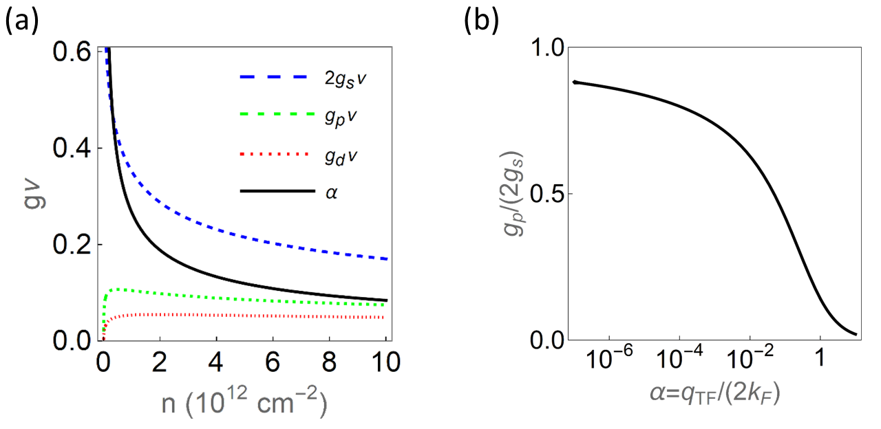
Two dimensions—Examples are electron hole bilayers and other 2D excitonic insulators such as monolayer WTe2 Jia et al. (2020). The natural pairing functions are which plugged into Eq. (S3) renders . Note that for , the factor should be changed to . Since and have the same , we will use the real pairing functions for convenience. For Thomas-Fermi screened interaction in 2D where is the ‘fine structure constant’ in this system and is the dielectric constant of the environment, the -wave pairing strength is
| (S4) |
and the -wave one is
| (S5) |
These equations were previously given Sun and Millis (2020b) and are reproduced here for convenience.
The pairing interactions are shown in Fig. S1 for the screened Coulomb interaction in 2D (reproduced from the supplemental material of Ref. Sun and Millis (2020b)). To obtain a substantial , one needs the high density case where the fermi velocity is large so that the Thomas fermi wave vector is smaller than the fermi momentum: . Stronger dielectric screening of the environment can further reduce and increase . Moreover, a non-negligible interlayer distance changes the bare electron-hole Coulomb attraction into , making it more nonlocal and thus can lead to a larger . Other types of interactions such as nearest neighbor Hubbard interaction (although originating from Coulomb) could give a very strong , given that the band overlapping is suitable.
II Computation of the polarization
In this section, we explicitly derive the charge pumping in an 1D excitonic insulator by computing the polarization (charge pumped) as a time integral of the current induced by adiabatic changes to the order parameter over a time interval from to and comparing the result to the formula in terms of Berry curvature, consistent with previous results King-Smith and Vanderbilt (1993).
II.1 Polarization
For convenience we reproduce the mean field Hamiltonian and current operator here:
| (S6) |
where is the velocity and the energy eigenvalues are . The current in response to a change in order parameter is
| (S7) |
in frequency representation where , are the Fermion and Boson Matsubara frequencies with (not to be confused with the carrier density), is the temperature and we have set the Boltzmann constant to be . Carrying out the trace over band indices, performing the frequency summation at and analytically continuing to , one obtains
| (S8) |
Note that if the argument is in , the latter means Fourier transformed into frequency representation. In the adiabatic limit we may neglect the in the denominators; then transforming to the time domain we obtain
| (S9) |
where ‘’ now means the expectation value of the current operator. Integrating in time gives the change in polarization:
| (S10) |
II.2 Berry Connection and Berry Curvature
The Berry connection is given in terms of the change in wave function under infinitesimal variation of the parameters as . We suppress the momentum subscripts whenever possible without causing ambiguity. Defining we may write the valence band wave function as
| (S11) |
implying where . Explicitly,
| (S12) |
Note that has singularities (“Dirac strings") along the line and also along the lines unless vanishes on parts of these lines. These are shown as dashed lines in Fig. S2(a) for the BEC case (). The Berry curvature is then
| (S13) |
Considering now the flux of through a surface element of an oriented 2D manifold in space defined by a function and choosing the orientation to be pointing ‘inside’ the cylinder in Fig. S2(a) we see by comparison to Eq. (S10) that the flux through the surface is just the polarization . This conclusion is independent of the choice of coordinate.
II.3 BCS-BEC crossover
If the numbers of electrons and holes are separately conserved, the total number is also conserved where is the particle number of a completely occupied band. is the analogy to the total charge in a superconductor, and gives the constraint that shifts from positive to negative as interaction becomes stronger such that the system crossovers from a BCS to a BEC type condensate. This is the situation in electron hole bilayers with no interlayer tunneling. Moreover, can also be approximately fixed by gate voltage. For natural crystals, is not fixed since there are always interband conversion mechanisms breaking this symmetry. Hartree terms due to Coulomb repulsion between a/b orbitals will shift down and induce such a crossover in this case.
In the BEC case (, no band inversion), there are no monopoles and the Dirac string structure looks like that in Fig. S2, rending zero pumped charge. Intuitively, the excitons in the BEC state are tightly bound electron hole pairs that don’t overlap with other, and can be viewed as charge neutral point particles. Thus no charge transport can occur.
Therefore, there is a topological transition at during the BCS-BEC crossover, and the charge pumping can be viewed as an ‘order parameter’ that separate these two regimes, as shown in Fig. S2(c). However, we have focused on the dynamics in the BCS limit in this paper while it is interesting to investigate similar dynamics in the crossover regime.
II.4 Pumped charge for arbitrary rotation angle
In this section we provide the details leading to Eqs. (5) and (6) of the main text. Parameterizing using and the angle defined in Fig. 1(a) of the main text, the Berry connection and curvature can be projected onto the space. In other words, The wave function can now be viewed as a function of and is the pairing field at . Note that reverses sign for positive and negative , and that is nearly zero deep inside the fermi sea () and outside when .
The flux can be converted to the line integral of the Berry connection over the edge of in Fig. 2(b) of the main text. The singularities (marked by crosses in Fig. 2(b)) are from the intersections with the Dirac strings, and must be correctly treated in the evaluation of the line integral, although they do not contain fluxes in . For a full cycle, the edge is the blue contour together with the two small circles surrounding the two vortices. The former gives zero net contribution due to periodicity in and while the latter contributes , recovering the number of monopoles.
The polarization at arbitrary angle can be evaluated analytically in the BCS limit in which where is the lattice constant. The Berry curvature is concentrated in the region so we may perform the integral in Eq. (3) of the main text only on the red rectangles centered on in Fig. 2(b) of the main text, chosen such that on the vertical edges inside the fermi momentum and thus from Eq. (S12), while on the vertical edges outside the fermi momentum and . The top and bottom edges all contribute zero since and thus are negligible around . Therefore, the contour integral gives
| (S14) |
for an 1D excitonic insulator. This result may also be understood by noting that the low energy physics around is of two massive Dirac models, each of which realizes a Goldstone-Wilczek Goldstone and Wilczek (1981) mechanism of charge pumping.
In a 2D system one has two momenta, which we choose to be parallel () and vertical to the direction defined by the antisymmetry of . The net charge pumped is then an integral over of the previously obtained formula. The only change is that now and it may be that for some values of the sign of does not change as a function of , meaning that for these the monopoles lie outside the torus of integration so no charge pumping occurs. In the weak coupling limit the issue may be discussed in terms of the Fermi surface of the metallic () phase. If the fermi surface (fermi crossings for each as is varied) is open the density of transferred charge is during a full cycle where is the lattice constant in direction; if the fermi surface is closed, then only the range of where crossings occur gives rise to a charge pumping; thus the net density of pumped charge during a full cycle is where is the maximum extent of the fermi surface in the direction.
In an isotropic 2D system, for an incomplete cycle with arbitrary , note that each 1D momentum chain crossing the fermi surface at contributes a charge pumping channel described by Eq. (S14), with effective rotation angle . Summing over all the chains, one obtains
| (S15) |
for . Extending the above integral to higher , one obtains Eq. (6) of the main text.
II.5 Current response in time domain
In this section, we try to expand Eq. (S7) to higher orders in frequency and show that this won’t give corrections to the adiabatic result. We focus on the nodes at in 2D when the system is close to pure -wave order. In 3D, the nodes become a nodal line and the result stays the same up to some constants. Close to , the trajectory of motion is nearly along the direction due to the saddle point structure on the free energy landscape in Fig. 4(a) of the main text. Thus it is enough to consider the current response to in Eq. (S8): . We assume the order parameter passes the point with nearly constant velocity . In the BCS limit, the second term vanishes due to the factor and what remains is
| (S16) |
where
| (S17) |
is the adiabatic current leading to Eq. (S15) and is a dissipative term that arises from quasiparicles excitations. At exactly , it is
| (S18) |
Another source for dissipative current is the quasiparticle contributed optical conductivity from the node:
| (S19) |
Its real part is suppressed by the small number and can thus be neglected.
It appears from Eq. (S18) that there is a correction to the pumped charge as . However, if one includes higher order terms in frequency, the current response from Eq. (S16) can be written in time domain:
| (S20) |
where
| (S21) |
is the response kernel which is time dependent due to the fact that , changes with time. Note that in the above integrals although we neglected its subscripts for notational simplicity. If one uses the values of at and evaluate the polarization at by , one recovers exactly the adiabatic current and the topological charge pumping. Therefore, the non-adiabatic correction is beyond the scope of Eq. (S21), but lies in the fact that the state at is not the ground state of the instantaneous mean field Hamiltonian assumed here. We will show that this physics can be addressed in terms of exact dynamics of pseudo-spins.
III Edge states
In this section we analyse the behavior of edge states. For simplicity we foucs on the weak coupling BCS limit of Eq. (S2) with open boundary condition. Linearizing the Hamiltonian near the two fermi points , we find that an edge state wave function may be written
| (S22) |
with energy where and we have made use of our convention . The spinor part of the wave function is
| (S23) |
To satisfy the open boundary condition , one requires which yields
| (S24) |
This and the relation is satisfied by two solutions: and . The corresponding wave functions are
| (S25) |
Note that the subscript tracks each wave function smoothly as varies, but does not specify either the energy or the side where the state is localized at. They are determined by the signs of their energies and the exponential factors.
The relation between the two edge states follows from symmetries. One may define two unitary operations, the ‘phase rotated inversion’ and the . Both operators inter converts the two edge states. is a symmetry of the mean field Hamiltonian if the system is in a pure -wave state while always anti commutes with . Therefore, have opposite energies and will be at zero energy in a pure -wave state.
Note that in open 1D wires connecting two reservoirs in Fig. 3 of the main text, although the edge states seem to be responsible for the charge pumping, the actual carries are all electrons in the valence band moved by continuous deformation of their wave functions, which is a bulk property. Indeed, in macroscopically long wires, the expansion and shrinking of edges states happen only in a tiny vicinity of , while the charge pumping is a continuous process as varies. For example in the state, although there is an occupied edge state localized on the right, the other electrons in the valence band form a density distribution that has a ‘hole’ on the right, such that the total polarization is still nearly zero. In the state, the background density distribution has a ‘half’ hole on each edge. Together with the occupied edge state on the right, it look like there is a half charge on the right edge and a half hole on the left, so that the polarization .
IV The Ginzburg-Landau action
In this section we present the derivation of the semiclassical action used in the main text. The Ginzburg-Landau action for order parameter fields and the EM field is obtained by integrating out the fermions () in Eq. (S2), resulting in
| (S26) |
The means trace of logarithm of the infinite dimensional matrix where should be interpreted as the spatial derivative acting on the fermion fields, i.e., the matrix is just the kernel for all Fermion fields at all in Eq. (S2) (See Sec. 6.4 of Ref. Altland and Simons (2010)). Performed in Fourier basis, it involves a summation over momenta , the fermion Matsubara frequencies (, is the temperature and we have set the Boltzmann constant to be ) and a trace of logarithm of the matrices. Note that we have removed the absolute value symbol from Eq. (S2) since are real numbers. We interpret the action as the Lagrangian for the order parameter fields moving in the presence of electric field . Changing the argument to , we write the Lagrangian
| (S27) |
as the sum of three terms: the static free energy landscape , the ‘Kinetic energy’ and drive terms. We consider each in turn.
IV.1 Static free energy landscape
By integrating out the fermions for static Hubbard-Stratonovich fields in Eq. (S26) we obtain the free energy density (see Ref. Sun et al. (2020) or Sec. 6.4, page 276 of Ref. Altland and Simons (2010)):
| (S28) |
where now means the trace of logarithm of the matrix at momentum . Note that the momentum integral has an ultraviolet (UV) cutoff which is at the order of fermi energy but also affected by the Thomas-Fermi screening length Kozlov and Maksimov (1965). Converting the integral variable to an energy , we find for (quasi) 1D systems in the BCS limit:
| (S29) |
For a 2D isotropic Fermi surface, the first term is replaced by
| (S30) |
where runs from to . In 3D, one just needs to make the replacement where is the polar angle ranging from to and is the azimuthal angle ranging from to . In 2D, as long as Sun and Millis (2020b), the -wave phase at is the ground state with energy while the -wave phase at is a saddle point that has energy . For , the ground state minimum shifts to an one. Note that in d dimensions, the density of states is where is the surface area of the dimensional sphere with radius . For example, in 2D, and .
IV.2 Kinetic energy
The action for order parameter fluctuations is obtained by expanding Eq. (S26) as
| (S31) |
around the mean field configuration to second order in , , temporarily neglecting the EM field. We assume spatially uniform, time-dependent order fluctuations and find the fluctuation term
| (S32) |
For convenience we will include the in the definition of and in this subsection. Evaluating the frequency integral at , taking the trace explicitly, rearranging and keeping only the terms with dependence gives
| (S33) |
Writing with the angular coordinates on the contours of constant energy, one obtains
| (S34) |
Defining we find for the energy integral
| (S35) |
In the adiabatic limit (lowest order in expansion), the kinetic energy is thus
| (S36) |
where . In 1D, writing , the kinetic term becomes
| (S37) |
If is very small and the system has a closed Fermi surface in or then the adiabatic expansion breaks down in the regions where the gap vanishes. In this case the operator becomes nonlocal in time, and the physics is most efficiently treated directly from the action Eq. (S2).
IV.2.1 Dissipative terms
For convenience, we first introduce the general form of correlation functions at zero temperature:
| (S38) |
where . We re-derive the kinetic terms by expanding the order parameter correlation functions in frequency:
| (S44) |
where the subscripts of the correlation functions correspond to their channels in . For example, which is Eq. (S38) with replaced by everywhere. The term in is
| (S47) |
where , , and is the angular variable in -dimension. The term is
| (S50) |
The term is
| (S53) |
The above expansions in fails as , the minimal gap around the fermi surface, especially when such that there are nodes at in 2D. We next evaluate the kernels in the pure -wave case to gain a rough idea of the crossover of dynamical behavior. The dissipative part of kernel is
| (S54) |
where is an infinitesimal positive number and we have made use of the quasi-particle density of states due to the nodes: . The linear in frequency dissipation continues with a cutoff of about beyond which it scales as a constant. Kramers-Kronig relation implies that
| (S55) |
The dissipative part of kernel is
| (S56) |
and the cubic behavior has the cutoff . This together with the limit of Eq. (S50) gives
| (S57) |
IV.2.2 In time domain
With the adiabatic approximation so at time we can write , the action from Eq. (S31) reads
| (S58) |
where is the retarded kernel in time domain as a matrix and in this subsection. The instantaneous (force) term in the Euler-Lagrange equations comes from the equal time correlator (potential) and the dynamics comes from expanding in derivatives, in other words
| (S59) |
Noting that we have
| (S60) |
The adiabatic approximation is reasonable if the change in over a time corresponding to the range of is small () so that we can evaluate at fixed . If we have a fully gapped configuration (open Fermi surface or not small), decays on times larger than so we can shift the derivative to the and integrate by parts to get
| (S61) |
with . However, for closed Fermi surfaces, the vanishing of at some Fermi surface points means that when is small has a part that decays slowly, actually on the time-scale of and a more careful analysis is needed. In the isotropic 2D case, we have
| (S62) |
and the (retarded) correlator is given by
| (S63) |
where is the Heaviside step function. Performing the integral over momentum, one obtains the low energy kernel
The off diagonal terms don’t affect the qualitative dynamics which we neglect. At small we can neglect the second term of . Therefore, in 2D, a smooth crossover between non dissipative and dissipative behaviors during the swiping across can be described by the retarded Kinetic kernel
| (S65) |
Eq. (IV.2.2) implies the equation of motion
| (S66) |
which describes the dissipationless-dissipative crossover behavior when crosses zero during the dynamics.
IV.3 The drive term
In the drive term , the linear coupling of electric field to the polarization is obvious. We derive the second term in this section. The kernel of the term is Sun and Millis (2020b)
| (S67) |
where is the current operator in Eq. (S6) and is the electron mass in our model. Since the second term in the current in Eq. (S6) is suppressed by the factor in the BCS limit, its contribution can be neglected. In 1D, the current correlation function is thus
| (S68) |
where and . The constant term cancels the diamagnetic contribution and what remains in the kernel is the term that corresponds to the static polarizability from ‘scattering states’ of the electron hole pair. In 2D, the current correlator up to is
| (S69) |
Therefore, the term in the action reads
| (S72) |
where the coefficient can be interpreted as . The higher order terms is are in higher powers of where is defined in the main text.
V The adiabatic transport scheme
V.1 Description
If the sin pulse is wide enough in time, it is possible to make the dynamics perfectly adiabatic since the system simply follows the instantaneous minimum on the free energy landscape. As the field increases, the minimum shifts away from counter clockwisely while the maximum at shifts clockwisely. The maximum field needed is simply that making the instantaneous minimum and maximum coincide. In 1D, this field can be computed analytically:
| (S73) |
where and . After reaching the maximum value (a little higher than that), the field starts to decrease, shifting back the two extrema. The order parameter is moved to the immediate left of the maximum, which gradually shifts back to as the field decreases to zero. The second half of the sin pulse would therefore transport the order parameter to the minimum at , completing a half cycle. However, if the decreasing field phase of the pulse is too slow, unstable fluctuations of order parameter tend to grow exponentiallySun and Millis (2020a) and get comparable to its mean field value within the ‘spinodal time’ where is the Ginzburg parameter of the landau theory. Therefore, the time scale of the pulse has to be smaller than the spinodal time.
If is too small, the requires maximum field is so large that the term would pull the order parameter to the origin and destroy the above adiabatic trajectory. This imposes an lower bound for the -wave pairing strength . For the adiabatic transport scheme to work, has to be larger than . These conclusions apply qualitatively to higher dimensions.
If the adiabatic scheme is realized, experimental measurement of the threshold electric field gives the estimation of through Eq. (S73). In the fast scheme described in the main text, if the full frequency spectrum of the current can be measured, it is possible to reconstruct the angular dynamics through, e.g., Eq. (6) of the main text.
V.2 Derivation
In 1D, incorporating the effect of a static electric field up to , the free energy is
| (S74) |
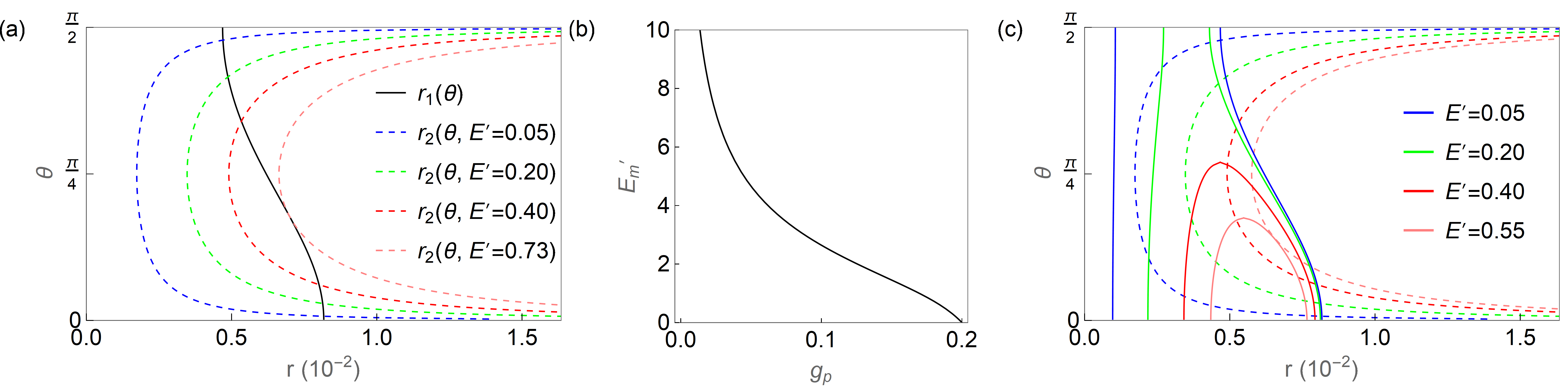
where the ‘polar’ coordinate is defined as , the dimensionless electric field is , and . Note that is in the main text. We look for saddle points on the free energy landscape within the domain . There are two curves defined by and respectively, whose solutions read
| (S75) |
where , as shown in Fig. S3(a). Note that we temporarily neglected the terms in the free energy. The intersections of the two curves are the saddle points. At zero field, the two saddle point are just the two minima at . For weak field, the two saddle points shift towards each other in angular direction. As the field further increases to the critical value , the two saddle point meet which means the two lines are tangent to each other: is satisfied at the intersection. This condition gives the angle at intersection as and critical field
| (S76) |
It increases from zero as decreases from , and diverges as as , as shown in Fig. S3(b).
The term in Eq. (S74) lowers the energy dramatically close to , and therefore tends to pull the system to the zero order state. As a result, the free energy has a maximum in the direction, followed by the minimum as increases. Thus the curve has two branches: the left one has (maxima) while the right one has (minima), as shown by the solid curves in Fig. S3(c) for weak fields. For strong enough field , it can happen that the two branches meet each other at certain such that there will be no saddle points along if , as shown by the solid curves in Fig. S3(c) for stronger fields. The summits of those curves satisfy which yields
| (S77) |
Making the summit at , the pure -wave order line, one obtains the minimal field for the curves to be closed, i.e., for the minima in direction to disappear at certain angles.
As the field increases, the intersections between the curve and the right branch of curve moves towards each other. If they successfully meet each other at certain field , the order parameter is handed by to and the subsequent decreasing field phase pushes back to the -wave order, i.e., adiabatic transport works. However, if is too weak, it can happen that annihilates with another intersection on the left branch of . In this situation, the order parameter will be transported to zero order instead of to the -wave state. The critical -wave pairing strength can be estimated roughly in this way: the summit of collides with the left most point of as field increases. This condition leads to the equality which renders .
VI Exact mean field dynamics
VI.1 Pseudo spin representation
The degree of freedom at each momentum in Eq. (2) of the main text can be mapped to an Anderson pseudo spin . In the second quantized language, each momentum labels two single particle states from the two bands whose annihilation operators are and , giving a 4-dimensional Hilbert space. However, the mean field dynamics here implies that the total occupation number at is always one ( commutes with the Hamiltonian) where and is the identity matrix. Therefore, it is enough to consider a 2-dimensional subspace of single occupancy which can be mapped to a pseudo spin- defined as where are the three Pauli matrices.
The general mean field Hamiltonian at momentum can be written as
| (S78) |
and the dynamics implied by Eq. (1) of the main text is mapped to the procession of the Anderson pseudo spins in the time dependent self consistent mean field Barankov et al. (2004):
| (S79) |
where the last equality is known as the gap equation. The EM vector potential enters by and we use a phenomenological damping to account for the effect of energy loss due to, e.g., the phonon bath. Starting with the ground state with a real , we simulated the dynamics induced by a pulse and the current is integrated over time to obtain the pumped charge. Some numerical solutions to Eq. (S79) are shown in Figs. S5 and S6.
Note that Eqs. (S78) and (S79) are general which allows for appearance of imaginary components of and . However, as a result of an emergent ‘particle-hole’ symmetry in the BCS weak coupling case that maps to , the order parameter dynamics is restricted to the plane where are always real numbers which we prove in the next subsection. Away from BCS weak coupling, the order parameter trajectory departs from the plane in a continuous way: e.g., can temporarily develop an imaginary component that couples to and can have an imaginary component that couples to . However, since the initial and final states are the same ones, and the charge pumping is still quantized for 1D systems because it is a topological effect.
VI.1.1 Proof of why the dynamics is confined within the plane in the BCS weak coupling case
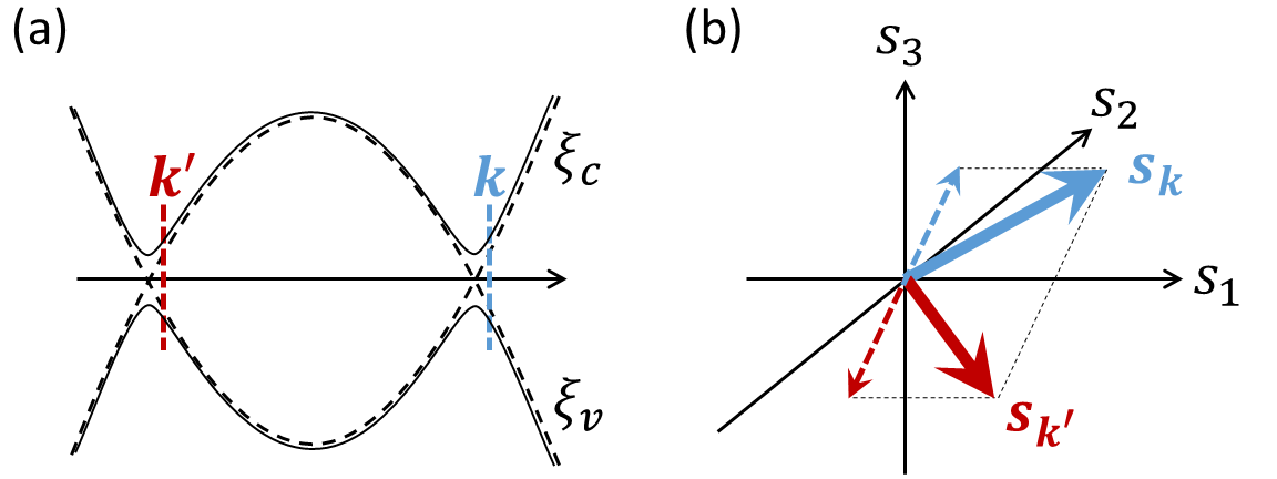
The physical argument is that in the BCS weak coupling case, there will be no force pushing the order parameter away from the plane during the dynamics. Following we provide a more mathematical proof. Define the ‘particle-hole’ operation
| (S80) |
where is the magnitude of Fermi momentum, is the unit vector along the direction of and we have used bold fonts for the momentum to emphasize its vector nature (although every in the main text and supplemental material already means a vector). The operation changes to its ‘particle-hole’ image , as illustrated in Fig. S4. In the BCS weak coupling case (), what is relevant are the low energy states close to the Fermi surface (band crossing point) where becomes a symmetry of the action in Eq. (1) of the main text (note that ). Considering that in the BCS weak coupling case, is changed to its complex conjugate under operation of according to Eq. (S80) and Eq. (S78). Therefore, given a solution to the order parameter dynamics, its ‘image’ must also be a solution. Given the initial condition of =, since the solution is unique, the order parameter trajectory must lie within the plane of , i.e., the plane studied in the main text.
An alternative way to prove this is using the pseudo-spin language. According to Eq. (S79), to prove that is always real, we just need to prove and are always related to each other by the ‘mirror’ operation with respect to ‘’ plane: , as shown in Fig. S4(b). Note that the pseudo spins are defined as axial vectors such that the mirror operation transforms the spins as . For the initial ground state, this is obviously true and the ‘magnetic field’ on the two pseudo-spins are also mirror images of each other under , so are . Therefore, this ‘mirror’ relation between the pseudo spins at is sustainable during the dynamics according to Eq. (S79), and guarantees that the order parameter stays on the plane.
VI.2 ‘Super-current’ in 1D systems
The solution is trivial in the degenerate case in the BCS limit where the effect of the pairing function is captured by on the right/left fermi point. We start from a ground state where all spins are pointing in plane: . Consider the electric field pulse at applied through . The leading driving term due to electric field is where around the right/left fermi point. The diamagnetic term is subleading in driving the spinor dynamics but contributes a diamagnetic current we will discuss in the end. After the kick, the spinors start to rotate around the ‘’ axis with angular frequency . The mean field rotates at the same speed: such that is always parallel to each spinor, not affecting the spin rotation. Thus the solution is that each spin synchronize and keeps rotating around ‘’ with angular frequency . Now we evaluate the current . The paramagnetic current vanishes in this state. The diamagnetic current is . Therefore, the system behaves like a ‘superconductor’ with the superfluid density .
VI.3 Dynamics of the node in 2D: Landau-Zener formula
The node contribution to the polarization is captured by a Dirac Hamiltonian with time dependent gap:
| (S81) |
which is an approximation to Eq. (2) of the main text around , and is valid for . Taking into account the higher order term in the Hamiltonian, the current in direction is . In the BCS limit we are concerned here, during the dynamics, the spinor at is always the mirror image (under defined in Sec. VI) of that at with respect to the plane. Therefore, the contributions to the current will always sum to zero, and it is enough to consider . Define the energy variables , , the Hamiltonian becomes
| (S82) |
and the current reads . We now use Eq. (S82) to study the spinor dynamics and the current generated.
As the order parameter passes the point with nearly constant velocity, the nodal gap changes sign. For the spinor at certain , as swipes from the positive value at time to negative value at time , the energy splitting starts from , passes through the minimal splitting , and ends up with . If the initial state is the low energy state, the probability of finally tunneling into the high energy state is given by the Landau-Zener formula Wittig (2005):
| (S83) |
which is exact if . Therefore, the tunneling probability is unity at the node and decays to zero away from the node within a range of . Considering there are two nodes, the total number of quasiparticles excited is thus
| (S84) |
Since we have assumed Dirac dispersion in the integral, Eq. (S84) is accurate if .
VI.3.1 The pumped charge around the node
We now compute the pumped charge, which reads
| (S85) |
The integral is completely determined by the dynamics governed by Eq. (S82), the evalution of which requires more detailed analysis of the time evolution of each spinor. Before that, we can guess the result simply from dimensional analysis. The nonadiabatic correction comes from spinors with , and the contribution arises during the anti crossing time regime when is not much larger than . Therefore, neither the momentum cutoff nor the maximum value of should enter the result. The only remaining energy scale in Eq. (S82) is provide by which has the unit of energy squared. Since the integral in has the unit of energy squared, one obtains where is a universal constant.
Now we compute exactly. It is more convenient to perform a permutation of the Pauli matrices: such that the node Hamiltonian reads
| (S86) |
and the current becomes . The dynamics of the pseudo spin at is a Landau-Zener problem Wittig (2005). At time , we have and the spin is in the ground state: . The time evolution can be written as where should not be confused with that from Sec. II. The Schrodinger equation for the amplitudes reads
| (S87) |
which leads to
| (S88) |
The current involves the expectation value of :
| (S89) |
whose time integral gives the charge:
| (S90) |
It can be seen from Eq. (S88) that the time dependent wave function is the same between the spins at and . Since the current is , the second term in Eq. (S90) will be canceled out by the two spins. The first term just needs the initial and final state information:
| (S91) |
which is provide by the Landau-Zener formula. Summing over all the spins, the pumped charge reads
| (S92) |
where the nonadiabatic correction is identified as
| (S93) |
Due to the negative relative sign of the non-adiabatic correction to the adiabatic one, we conclude that
| (S94) |
Therefore, Eq. (S94) gives the non adiabatic correction during each half cycle of order parameter rotation, which is valid if . This formula is nonperturbative in the swiping speed in the sense that, it can not be obtained by integrating over instantaneous linear or nonlinear current response functions perturbatively over the time evolution.