TOI-1736 and TOI-2141: two systems including sub-Neptunes around solar analogs revealed by TESS and SOPHIE††thanks: Based on observations collected with the SOPHIE spectrograph on the 1.93 m telescope at the Observatoire de Haute-Provence (CNRS), France.
Planetary systems around solar analogs inform us about how planets form and evolve in Solar System-like environments. We report the detection and characterization of two planetary systems around the solar analogs TOI-1736 and TOI-2141 using TESS photometry data and spectroscopic data obtained with the SOPHIE instrument on the 1.93 m telescope at the Observatoire de Haute-Provence (OHP). We performed a detailed spectroscopic analysis of these systems to obtain the precise radial velocities (RV) and physical properties of their host stars. TOI-1736 and TOI-2141 each host a transiting sub-Neptune with radii of R♁ and R♁, orbital periods of d and d, and masses of M♁ and M♁, respectively. TOI-1736 shows long-term RV variations that are consistent with a two-planet solution plus a linear trend of m s-1 d-1. We measured an RV semi-amplitude of m s-1 for the outer companion, TOI-1736 c, implying a projected mass of MJup. From the GAIA DR3 astrometric excess noise, we constrained the mass of TOI-1736 c at MJup. This planet is in an orbit of d with an eccentricity of and a semi-major axis of au, where it receives a flux of times the bolometric flux incident on Earth, making it an interesting case of a supergiant planet that has settled into an eccentric orbit in the habitable zone of a solar analog. Our analysis of the mass-radius relation for the transiting sub-Neptunes shows that both TOI-1736 b and TOI-2141 b likely have an Earth-like dense rocky core and a water-rich envelope.
Key Words.:
stars: planetary systems – stars: individual: TOI-1736, TOI-2141 – stars: solar-type – techniques: photometric, radial velocity1 Introduction
Studying solar analogs is a way to understand the evolution of stars similar to our Sun. Although the physical and evolutionary stellar characteristics of solar analogs are relatively well studied, the formation and evolution of planetary systems around these stars still lack observational constraints.
The Sun being the nearest and most studied star, where the most accurate stellar properties can be obtained, provides a way to benchmark measurements of distant stars that have similar physical properties. This fact favors a specific class of stars called solar analogs, defined as those stars that have physical properties within a certain range of solar values. Soderblom & King (1998) defined a solar analog to be a main sequence star with an effective temperature between 5278 K and 6278 K, a metallicity within the range dex, and it must not have a close stellar companion (arbitrarily defined with an orbital period of less than ten days).
The motivation to study solar analogs lies in the fact that stellar properties can be obtained with a greater precision since the Sun can be used as a reference (e.g., Bedell et al., 2014; Ramírez et al., 2014). Consequently, the uncertainties of the physical parameters of exoplanets can be significantly reduced for the solar analogs, which makes them interesting laboratories to understand the physics of planetary systems. In addition, stellar abundances can be obtained with greater accuracy, which informs us about the chemical composition of the environment where the planets formed. As a result, chemical clocks (e.g., da Silva et al., 2012) can provide better age diagnoses that can be used to validate the isochronal ages. This can also improve, for example, the constraints in exoplanet interior structure models based on the abundance of refractory elements (Fe, Mg, and Si) of the host star (Dorn et al., 2015; Adibekyan et al., 2021). Ultimately, studying planets around solar analogs also makes our knowledge of the conditions for the development of life less uncertain.
The Transiting Exoplanet Survey Satellite (TESS, Ricker et al., 2015) has identified more than 6000 candidate exoplanets (Guerrero et al., 2021). The transit method is efficient to detect close-in planets. Long-term radial velocity (RV) programs, such as the one carried out with the SOPHIE instrument at the Observatoire Haute-Provence, can establish the nature of candidate planets identified by TESS and can also detect additional non-transiting companions. We have identified two exoplanet candidates detected by TESS around the solar analogs TOI-1736 (TIC 408618999) and TOI-2141 (TIC 287256467). These planet candidates were identified as a TESS object of interest (TOI), which presented recurrent transit-like events in their light curves (Jenkins, 2002; Jenkins et al., 2010). Our RV follow-up with SOPHIE characterizes the nature of these two planets and detects at least two additional companions in the system TOI-1736. This paper presents the detection and characterization of both systems, where we performed a detailed analysis of their spectra to obtain a refined characterization of the host stars. The stellar parameters are summarized in Table 1. We combined the TESS and RV data to characterize all planets in both systems. Finally, we present an analysis of the internal structure and possible compositions of the innermost planets.
| Parameter | TOI-1736 | TOI-2141 | Ref. |
| ID (TYC) | 4313-01054-1 | 1540-497-1 | |
| ID (TIC) | 408618999 | 287256467 | |
| RA (hh:mm:ss.ss) | 02:53:44.4053447688 | 17:15:02.9060957472 | 1 |
| Dec (dd:mm:ss.ss) | +69:06:05.066418744 | +18:20:26.764729476 | 1 |
| Epoch (ICRS) | J2000 | J2000 | 1 |
| proper motion in RA, (mas yr-1) | 1 | ||
| proper motion in Dec, (mas yr-1) | 1 | ||
| parallax, (mas) | 1 | ||
| distance (pc) | 1 | ||
| B (mag) | 2 | ||
| V (mag) | 2 | ||
| TESS T (mag) | 2 | ||
| GAIA G (mag) | 1 | ||
| 2MASS J (mag) | 3 | ||
| 2MASS H (mag) | 3 | ||
| 2MASS K (mag) | 3 | ||
| WISE 1 (mag) | 4 | ||
| WISE 2 (mag) | 4 | ||
| WISE 3 (mag) | 4 | ||
| WISE 4 (mag) | 4 | ||
| effective temperature, (K) | this work | ||
| surface gravity, (dex) | this work | ||
| Fe metallicity, (dex) | this work | ||
| turbulence velocity, (km/s) | this work | ||
| bolometric flux, ( erg s-1 cm) | this work | ||
| star mass, (M⊙) | this work | ||
| star radius, (R⊙) | this work | ||
| luminosity, | this work | ||
| activity index, | this work | ||
| rotation velocity, (km s-1) | this work | ||
| rotation period, (d) | this work (5) | ||
| age (Gyr) | this work |
2 Observations
2.1 TESS photometry
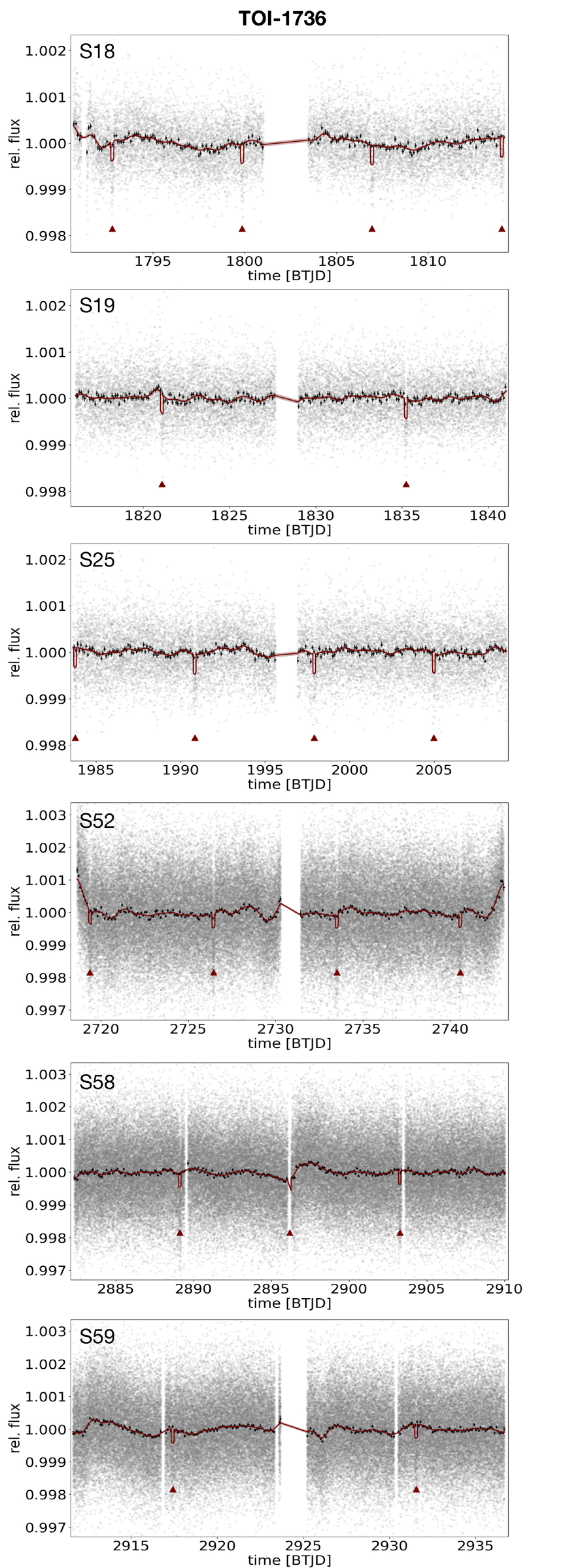
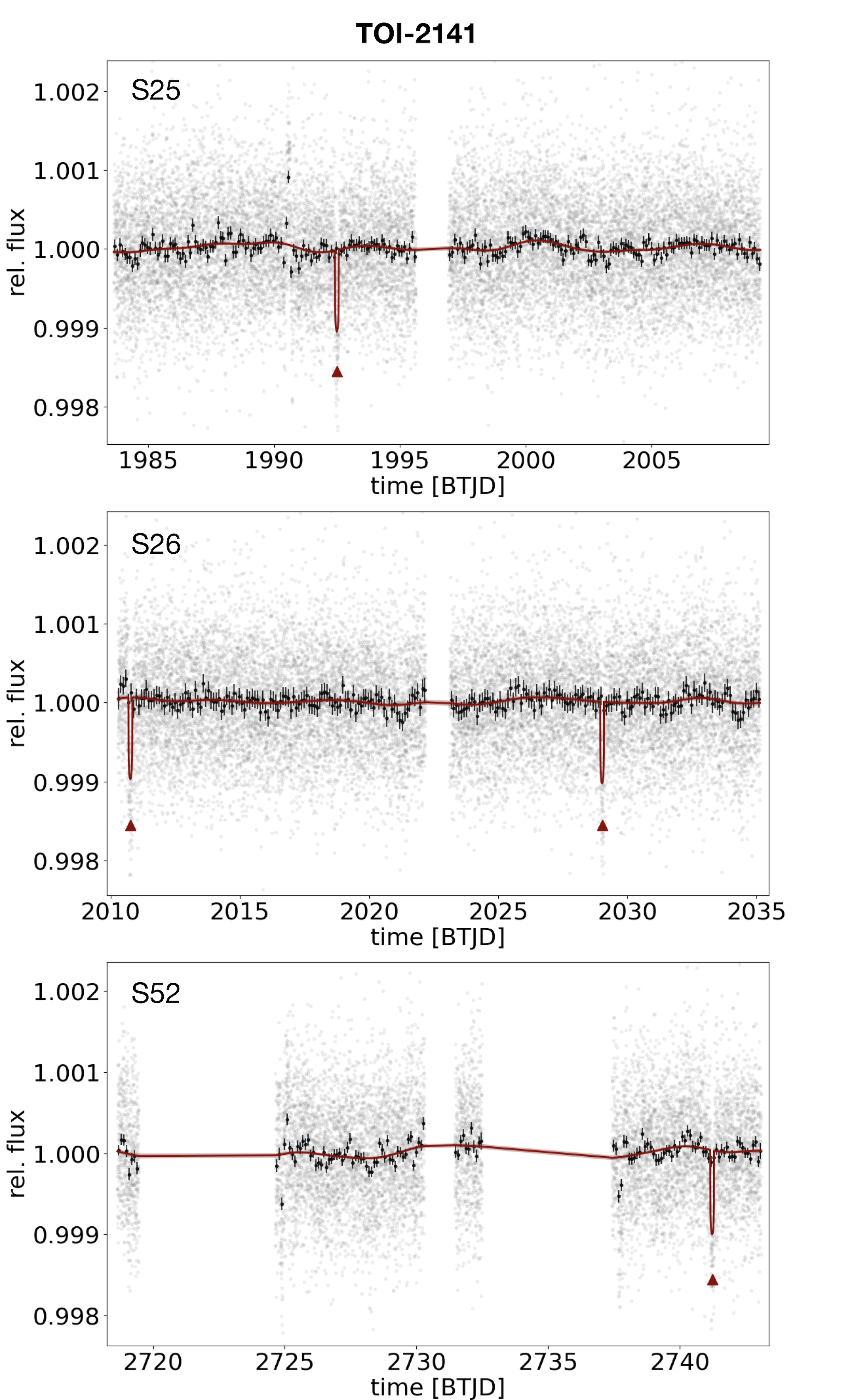
The TESS mission observed TOI-1736 with a cadence of 2 minutes in Sectors 18, 19, and 25, and with a cadence of 20 seconds in Sectors 52, 58, and 59. TOI-2141 was observed with a cadence of 2 minutes in Sectors 25, 26, and 52. Table 2 shows the log of TESS observations for these two objects. We obtained the TESS data products from the Mikulski Archive for Space Telescopes (MAST)222mast.stsci.edu, where we used the Presearch Data Conditioning (PDC) flux time series (Smith et al., 2012; Stumpe et al., 2012, 2014) processed by the TESS Science Processing Operations Center (SPOC) pipeline (Jenkins et al., 2016) versions listed in Table 2.
| OBJECT | TSTART (UTC) | TSTOP (UTC) | Duration (d) | Cadence | Sector | Cycle | Camera | SPOC version |
| TOI-1736 | 2019-Nov-02 | 2019-Nov-27 | 24.4 | 2 min | 18 | 2 | 2 | 4.0.29-20200410 |
| TOI-1736 | 2019-Nov-27 | 2019-Dec-24 | 25.1 | 2 min | 19 | 2 | 2 | 4.0.30-20200415 |
| TOI-1736 | 2020-May-13 | 2020-Jun-08 | 25.7 | 2 min | 25 | 2 | 4 | 4.0.36-20200520 |
| TOI-1736 | 2022-May-18 | 2022-Jun-13 | 24.4 | 20 s | 52 | 4 | 4 | 5.0.72-20220608 |
| TOI-1736 | 2022-Oct-29 | 2022-Nov-26 | 27.7 | 20 s | 58 | 5 | 2 | 5.0.78-20221129 |
| TOI-1736 | 2022-Nov-26 | 2022-Dec-23 | 26.4 | 20 s | 59 | 5 | 2 | 5.0.79-20221214 |
| TOI-2141 | 2020-May-13 | 2020-Jun-08 | 25.7 | 2 min | 25 | 2 | 1 | 4.0.36-20200520 |
| TOI-2141 | 2020-Jun-08 | 2020-Jul-04 | 24.9 | 2 min | 26 | 2 | 1 | 5.0.3-20200718 |
| TOI-2141 | 2022-May-18 | 2022-Jun-13 | 24.4 | 2 min | 52 | 4 | 1 | 5.0.72-20220608 |
The SPOC searches light curves for transiting planets with an adaptive, noise-compensating matched filter (Jenkins, 2002; Jenkins et al., 2010, 2020). The transit signatures of each candidate are fitted with an initial limb-darkened transit model (Li et al., 2019) and subjected to a suite of diagnostic tests (Twicken et al., 2018), all available in the TESS SPOC data validation reports (DVR). The DVR for TOI-1736 reports a candidate planet, hereafter TOI-1736 b, with an estimated radius of R R♁ and an orbital period of P d. The difference image centroid offsets locate the source of the transit signal within arcsec of the target star. The TESS Science Office (TSO) issued an alert for TOI 1736.01 on 27 February 2020 based on the DVR associated with the combined light curve for Sectors 18-19 (Guerrero et al., 2021).
The DVR for TOI-2141 reports two candidates, but only one passed validation tests. The unvalidated events have a periodicity of 30.6 d and are likely due to contamination by scattered light. We also note that the odd and even depth test supports a single strong feature folded on top of a much weaker and much less convincing transit-like feature for these events. The validated candidate planet, hereafter TOI-2141 b, has an estimated radius of R R♁ and an orbital period of P d. The centroid offsets localize the source of the transit signal within arcsec. The transit signature was first identified in the SPOC search of the Sector 26 light curve, and an alert for TOI 2141.01 was issued by TSO on 7 August 2020. Therefore, both TOI-1736 and TOI-2141 systems host at least one close-in transiting planet candidate with a size consistent with a sub-Neptune. Figures 1 and 2 depict the TESS photometry data for both respective objects.
2.2 LCOGT 1 m NEB Search
The TESS pixel scale is pixel-1, and photometric apertures typically extend out to roughly 1 arcminute, which generally results in multiple stars blending in the TESS aperture. To attempt to determine the true source of the TESS detection, we conducted ground-based photometric follow-up observations of the field around TOI-1736 as part of the TESS Follow-up Observing Program333https://tess.mit.edu/followup Sub Group 1 (TFOP; Collins, 2019).
We observed a full predicted transit window of TOI-1736 b in Pan-STARRS -short band using the Las Cumbres Observatory Global Telescope (LCOGT; Brown et al., 2013) 1.0 m network node at McDonald Observatory on UTC 2020 August 28. If the event detected in the TESS data is indeed on-target, the shallow SPOC reported depth of 380 ppm would not generally be detectable in ground-based observations. Instead, we slightly saturated TOI-1736 to enable the extraction of light curves of nearby fainter stars to attempt to rule out or identify nearby eclipsing binaries (NEBs) as potential sources of the TESS detection. The 1 m telescopes are equipped with SINISTRO cameras having an image scale of per pixel, resulting in a field of view. The images were calibrated by the standard LCOGT BANZAI pipeline (McCully et al., 2018), and photometric data were extracted using AstroImageJ (Collins et al., 2017).
To account for possible contamination from the wings of neighboring star point spread functions (PSFs), we searched for NEBs in all known Gaia DR3 and TICv8 nearby stars out to from TOI-1736 that are possibly bright enough in the TESS band to produce the TESS detection (assuming a 100% eclipse and 100% contamination of the TESS aperture). To attempt to account for possible delta-magnitude differences between the TESS band and the follow-up filter band, we checked stars that are an extra 0.5 magnitudes fainter in TESS-band than needed. We find that the RMS of each of the light curves of the 24 stars matching our criteria is more than a factor of 5 smaller than the expected NEB depth in the respective star. We then visually inspected each neighboring star’s light curve to ensure no obvious eclipse-like signal. All of our follow-up light curves and supporting results are available on the EXOFOP-TESS website444https://exofop.ipac.caltech.edu/tess/target.php?id=408618999. Through our process of elimination, we find that the TESS signal must be occurring in TOI-1736 relative to known Gaia DR3 and TICv8 stars.
2.3 High contrast imaging
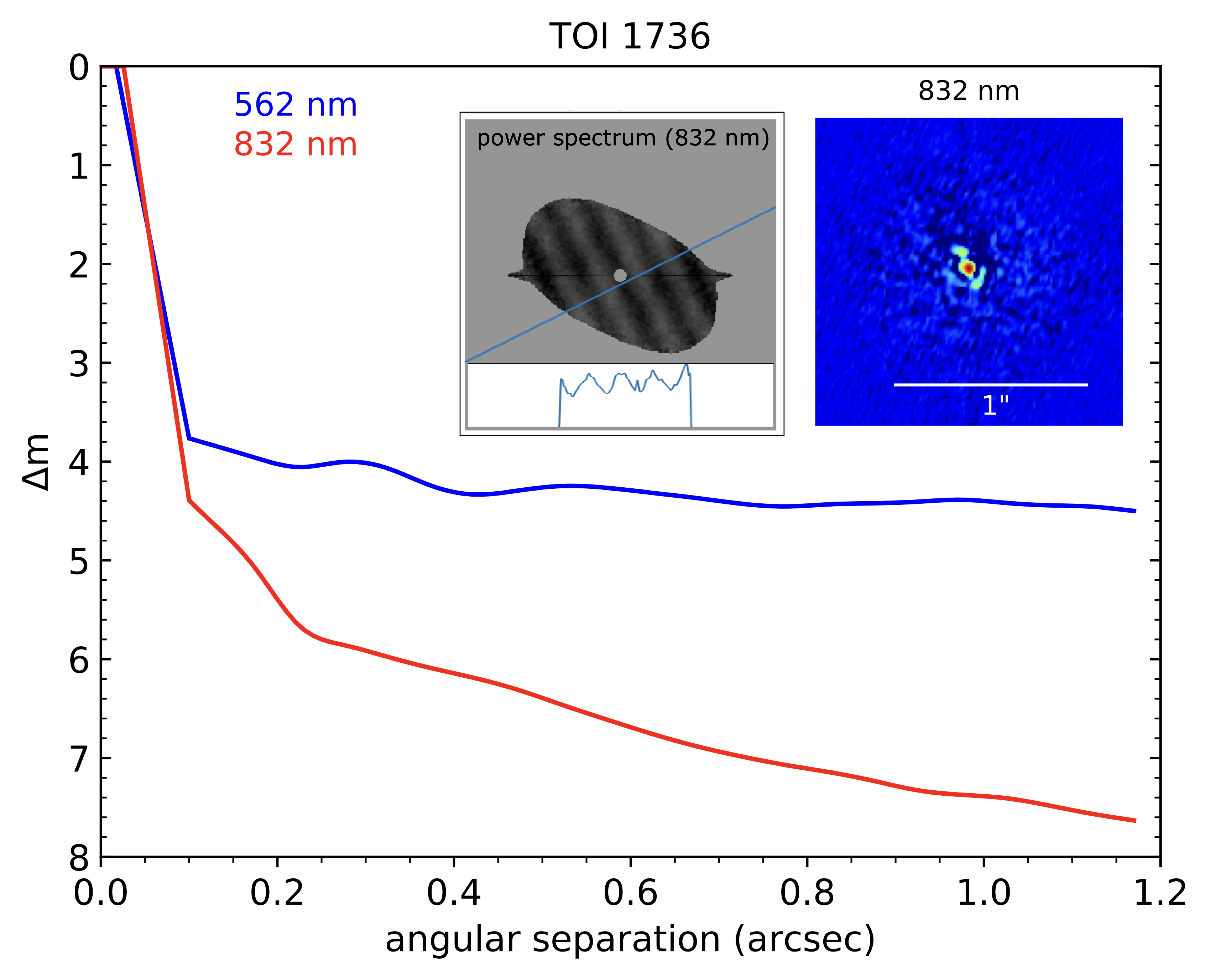
High-angular-resolution observations can probe close companions within arcsec that can create a false positive transit signal if that companion is an eclipsing binary, and which dilute the transit signal and thus yield underestimated planet radii (Ciardi et al., 2015). TOI-1736 was observed on October 19, 2021, by the ‘Alopeke dual-channel speckle imaging instrument on Gemini-N (PI: Howell) with a pixel scale of 0.01 arcsec/pixel and a full width at half maximum (FWHM) resolution of 0.02 arcsec. ‘Alopeke provided simultaneous speckle imaging at 562 and 832 nm. The data were processed with the speckle pipeline (Howell et al., 2011), which yielded the 5-sigma sensitivity curves shown in Figure 3. These observations provide a contrast at an angular separation of 0.5 arcsec of 4.2 mag at 562 nm and 6.4 mag at 832 nm. Figure 3 also shows the reconstructed image at 832 nm and its Fourier transform, which shows fringes in the power spectrum, evidence of a stellar companion to TOI-1736. The best-fit binary model for the power spectrum gives a companion at an angular separation of arcsec and position angle of deg with a magnitude difference from the primary of at 832 nm.
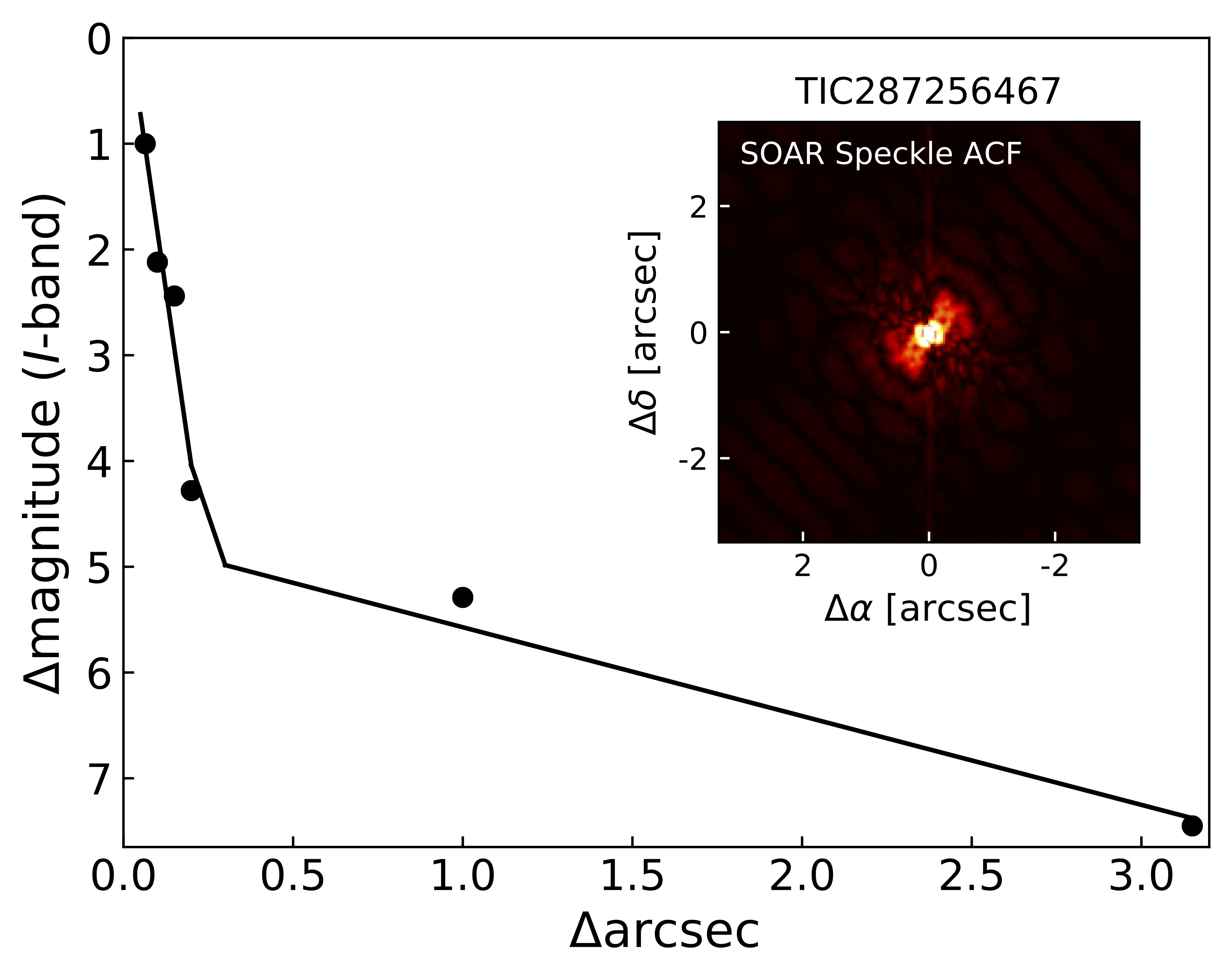
TOI-2141 was observed on April 25, 2021, with the 4.1-m SOAR telescope in speckle imaging. These observations provide a contrast of 5 mag at an angular separation of 1.0 arcsec in the I-band (Figure 4). These observations did not reveal any evidence of close stellar companions to TOI-2141.
2.4 SOPHIE spectroscopy
2.4.1 Observations
SOPHIE is a high-resolution fiber-fed, cross-dispersed échelle spectrograph mounted on the 1.93-m telescope at the Observatoire de Haute-Provence (OHP) (Perruchot et al., 2008; Bouchy et al., 2013). It covers a wavelength domain from 387.2 nm to 694.3 nm across 39 spectral orders. We observed TOI-1736 and TOI-2141 under a program dedicated to an RV follow-up of transiting candidates (e.g., König et al., 2022; Moutou et al., 2021; Hébrard et al., 2020), where we obtained 152 spectra of TOI-1736 between 2020-08-20 and 2023-03-11 with an average peak signal-to-noise ratio (S/N) per pixel at 550 nm of 70, and 90 spectra of TOI-2141 between 2021-02-25 and 2022-09-18 with an average peak S/N of 55. Both targets have been observed in the high spectral resolution mode (HR mode, R=75000) of SOPHIE. Tables LABEL:tab:sophiervstoi1736 and LABEL:tab:sophiervstoi2141 present more information about these observations.
2.4.2 Data reduction by the DRS
Our data have been reduced by the SOPHIE Data Reduction Software (DRS, Bouchy et al., 2009), excluding the seven first (redder) spectral orders due to their low S/N. Five spectra of TOI-1736 were not used due to their low overall S/N (below 40). The DRS automatically extracts and calibrates the spectra and computes the RV using the cross-correlation function (CCF) between the spectra and a G2-type empirical weighted numerical mask. The DRS also uses the CCF data to deliver stellar activity indicators, such as the CCF FWHM and the bisector span (BIS).
In order to improve the accuracy of SOPHIE measurements, we used the optimized procedures presented by Heidari et al. (2022) and Heidari et al. (in prep). This includes in particular: (1) CCD charge transfer inefficiency correction (Bouchy et al., 2013); (2) correction for the moonlight contamination using the simultaneous sky spectrum obtained from the second SOPHIE fiber aperture (e.g., Pollacco et al., 2008; Hébrard et al., 2008); (3) RV constant master correction for instrumental long-term drifts (Courcol et al., 2015); and (4) correction of the instrumental short-term drifts thanks to the frequently measured drifts interpolated at the precise time of each observation.
2.4.3 The CCF analysis by sophie-toolkit
In addition to the DRS reduction, we implemented an independent CCF analysis using the methodology described in Martioli et al. (2022), where we developed the Python package sophie-toolkit555https://github.com/edermartioli/sophie to obtain the RVs and other CCF quantities from a set of reduced SOPHIE spectra (both in the e2ds or s1d formats provided by the DRS). Our CCF approach is fundamentally the same as that applied by the DRS and therefore it should produce equivalent results. We compared the RVs from both CCF analyses, and despite some systematic effects in a small fraction of the data, they mostly agree within the error bars. As explained in Section 2.4.2, the DRS implements additional procedures to optimize the RV measurements in the SOPHIE data, which ultimately provide more accurate RVs. Thus, in our analysis, we adopted the DRS RVs.
The analysis performed by sophie-toolkit was originally designed for near-infrared observations with the SPIRou spectrograph (Donati et al., 2020), where it implements some processing steps that are aimed at mitigating the strong effects of telluric contamination and detector artifacts. Such analysis is more robust to systematics and improves some results when applied to the SOPHIE optical spectrum, where the aforementioned effects are much less significant, but still present in the data. An important step that is applied in our tool is an iterative registration of the spectra, both in flux and wavelength domains, to match each observation to a high S/N template stacked spectrum (“template” hereafter). Registration is done by shifting the spectra to the same topocentric frame using the precise RV values obtained from the CCF analysis and by scaling the fluxes using an order-by-order least squares fit to a third-order polynomial (see Martioli et al., 2022). This reduces residual systematic errors between observations, providing a differential measurement of each spectrum with respect to the template. This procedure also provides the dispersion in flux for each spectral element along the time series, which allows us to estimate statistical errors and assign proper weights to the data before performing measurements such as CCFs, RVs, and spectral indices. In addition to the CCF and RV data, sophie-toolkit provides other important products, such as the template spectrum, obtained from the median stack of all spectra in the time series. This product is saved in FITS format to store both the template and all other registered spectra. The most relevant activity indicators are also calculated and saved in a time series product, as detailed in Section 3.6. The Appendix A presents the final RV data (from the DRS) together with the corresponding spectral quantities obtained in our analysis using the sophie-toolkit package, all compiled in Tables LABEL:tab:sophiervstoi1736 and LABEL:tab:sophiervstoi2141.
2.5 TRES spectroscopy
For spectroscopic reconnaissance, we obtained four spectra of TOI-1736 and two spectra of TOI-2141 using the 1.5 m Tillinghast Reflector Echelle Spectrograph (TRES; Fűrész et al., 2008) located at the Fred Lawrence Whipple Observatory (FLWO) in Arizona. The spectra for TOI-1736 and TOI-2141 were obtained between March 3 - October 4, 2020, and between August 17 - October 20, 2020. TRES is a fiber-fed echelle spectrograph with a wavelength range of 390-910 nm and a resolving power of R=44,000. Spectra were extracted and reduced as described in Buchhave et al. (2010).
3 Stellar characterization
We carried out an analysis of the spectral and photometric data of both systems to derive the host stars’ properties as is detailed in the next sections. A summary of the final star parameters is presented in the Table 1.
3.1 Spectral energy distribution analysis
We performed an analysis of the broadband spectral energy distribution (SED) of both stars including the Gaia Early Data Release 3 parallaxes (with no systematic offset applied; see, e.g., Stassun & Torres, 2021) in order to determine an empirical measurement of the stellar radius, following the procedures described in Stassun & Torres (2016), Stassun et al. (2017), and Stassun et al. (2018).
We performed a fit using NextGen stellar atmosphere models (Hauschildt et al., 1999), with the effective temperature (), metallicity ([Fe/H]), and extinction () as free parameters. The surface gravity () has little influence on the broadband SED.
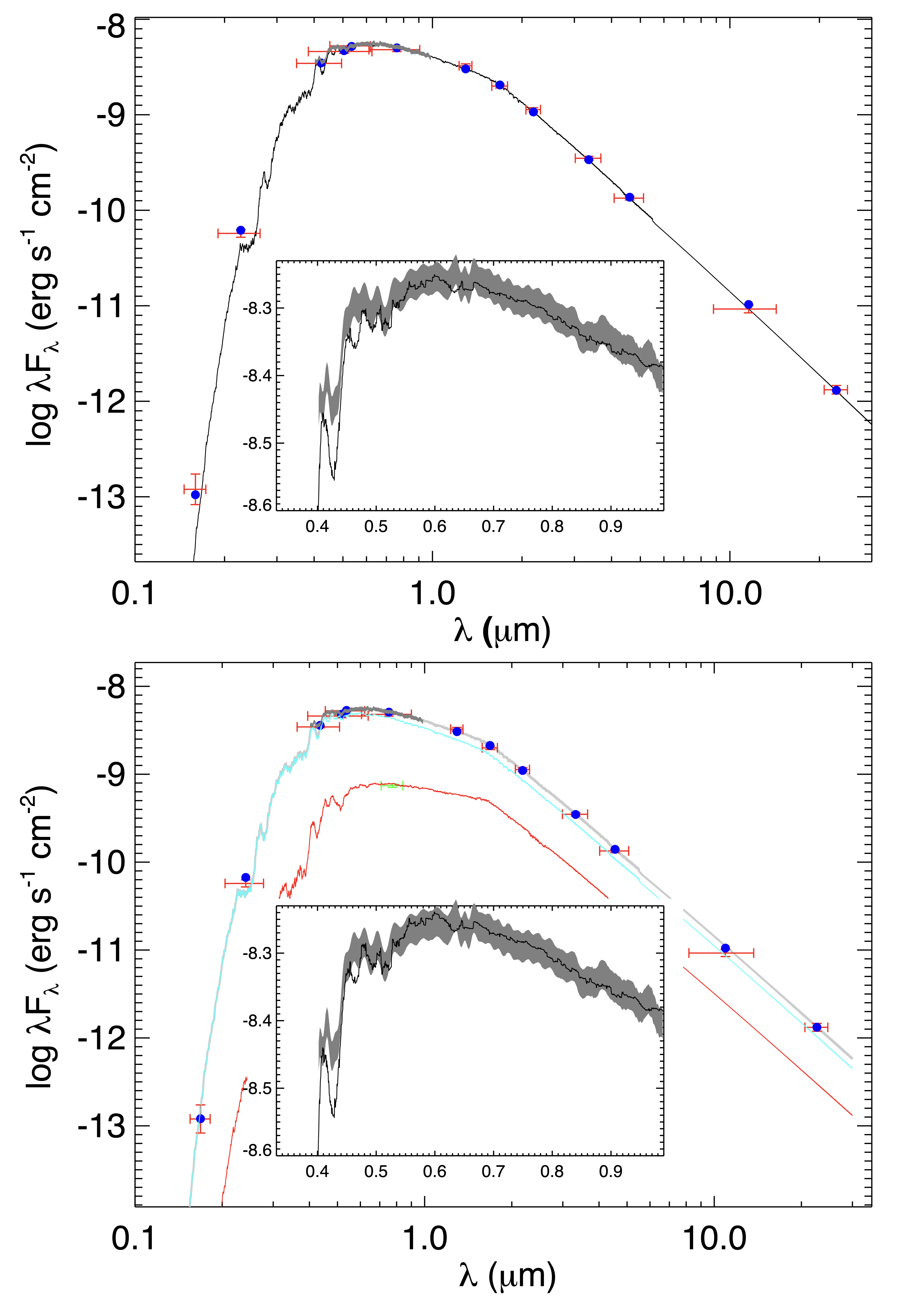
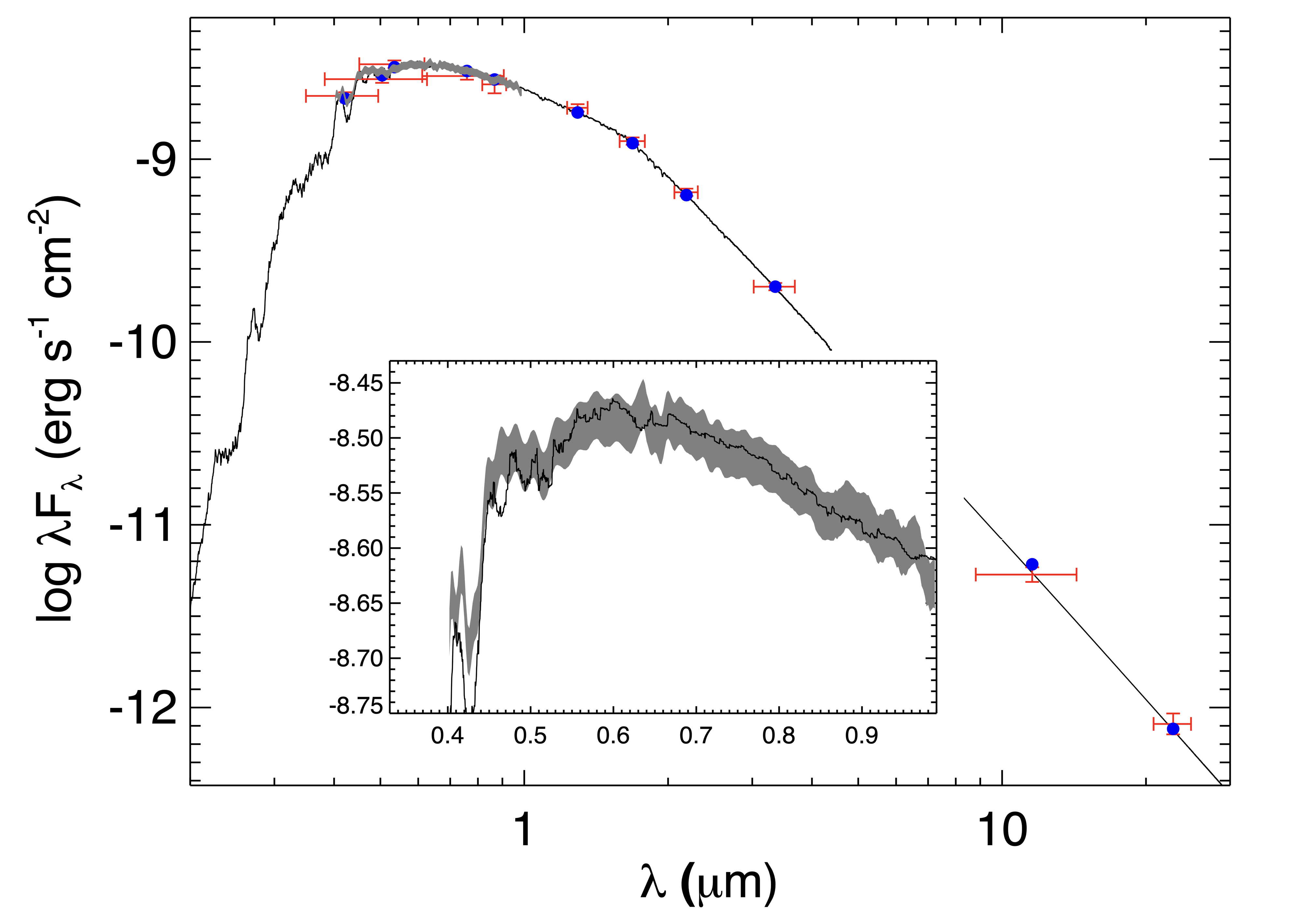
As a test to investigate whether the companion to TOI-1736 detected by the high contrast imaging results presented in Section 2.3 is real, we first fit a single-component model to the SED, as shown in the top panel of Figure 5, where we obtained a reduced of 1.1, with the best-fit parameters K, [Fe/H]=, and . According to the tool Stilism666https://stilism.obspm.fr/ (Lallement et al., 2014), the expected extinction for the distance of pc, galactic latitude and longitude from TOI-1736 is mag, therefore an abnormal reddening (or an infrared excess flux) was detected in our model. Then we consider a two-component stellar model to fit the SED of TOI-1736, assuming that the secondary has the same extinction () and metallicity as the primary. The bottom panel of Figure 5 shows these results, which give a of 1.0 with the same fit parameters for the primary and K for the secondary. Hence, the SED of TOI-1736 provides additional support to the binary hypothesis. For TOI-2141, we adopt a single-component model as illustrated in Figure 6, which gives a reduced of 1.3 and the best fit parameters K, [Fe/H]=, and .
Integrating the SED model gives the bolometric flux on Earth (), which can be combined with the and the Gaia parallax to derive the stellar radius. For TOI-1736, the single component model gives a radius of R⊙ and the two-component model gives a smaller radius of R⊙ for the primary and R⊙ for the secondary. For TOI-2141, we obtained a radius of R⊙. Using the mass-radius relations of Torres et al. (2010), we calculate the stellar masses of M⊙ for TOI-1736 and M⊙ for TOI-2141.
3.2 Standard analysis of SOPHIE spectra
To obtain the stellar parameters from the SOPHIE data, we constructed an average spectrum for both stars, using all SOPHIE spectra that were unaffected by the Moon’s pollution, and performed a standard spectral analysis on them. The average spectra of TOI-1736 and TOI-2141 have an S/N at 649 nm of 1100 and 850, respectively. We use the methods presented in Santos et al. (2004) and Sousa et al. (2008) to derive the effective temperatures , the surface gravities , and the metallicities . Using these spectroscopic parameters as input, the stellar masses were derived from the Torres et al. (2010) calibration with a correction following Santos et al. (2013). The errors were calculated from 10,000 random realizations of the stellar parameters within their error bars and assuming Gaussian distributions. The parameters obtained from this analysis are presented in Table 4 labeled as “standard.”
3.3 Spectroscopic parameters from TRES spectra
We use the reduced TRES spectra to obtain the stellar parameters using the Stellar Parameter Classification tool (SPC; Buchhave et al., 2012). In short, SPC correlates each observed spectrum against a grid of synthetic spectra based on Kurucz (Kurucz, 1992) atmospheric models and derives the effective temperature, surface gravity, metallicity, and rotational velocity of the star. The parameters obtained from this analysis are presented in Table 4.
3.4 Strictly differential analysis of SOPHIE spectra
We take advantage of the spectroscopic similarity between our targets and the Sun to apply a strictly differential analysis to determine atmospheric parameters and elemental abundances (e.g., Ramírez et al., 2014; Bedell et al., 2014). The differential analysis in such cases can potentially mitigate the Fe I/II excitation-ionization balance internal errors caused by possible differences in the micro-physics prescriptions, in the local determination of the continuum, or in the equivalent width (EW) measurements. Our reference solar spectrum was obtained from observations of the Moon with SOPHIE on 2023-04-01 with an S/N of 245 at 649 nm, maintaining the same instrumental configuration as the one used to observe the scientific targets.
We perform a line-by-line analysis with respect to the solar spectrum, which is based on the following steps. Given a narrow spectral range around each selected line, we normalize the stellar and solar spectrum using the same local continuum regions and then fit a Gaussian function to the solar line profiles, computing all resulting parameters (e.g., line depth, centroid, FWHM, and continuum offset). Then, we repeat the line fitting procedure for the locally normalized stellar spectrum, now fixing the continuum offset and line region information obtained from the respective solar spectrum. We employ the ionization-excitation equilibrium method where we adopted a line list from Meléndez et al. (2014), which contains excitation potentials, oscillator strengths, laboratory values, and hyperfine structure corrections777albeit it has a small impact on stellar abundances of solar analogs, in the Y II lines we corrected for this effect.. We included iron-peak, s- and alpha-capture elements, such as Fe, Mg, Al, Si, Ti, Y, and Ca to perform this spectroscopic analysis.
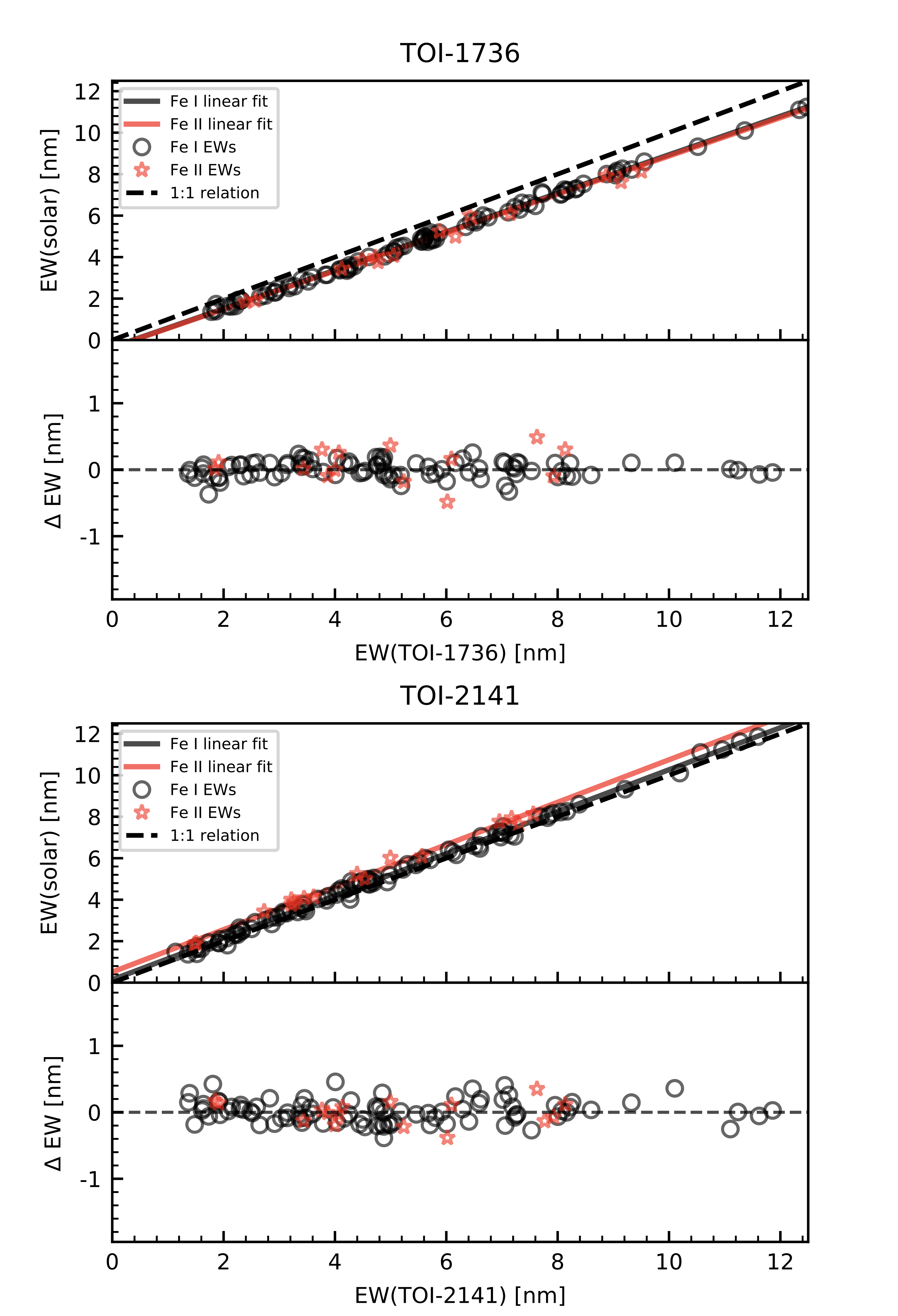
In Figure 7 we show the relationship between the solar Fe I and Fe II EWs and those of TOI-1736 and TOI-2141. The low scatter () for both stars indicates that the differential spectroscopic equilibrium analysis with respect to the Sun is sufficiently precise for the determination of the stellar atmospheric parameters. While not an exact match to our Sun, exercising caution and maintaining a conservative approach in considering uncertainties is warranted.
We use the code q2 (Ramírez et al., 2014) to model both the stellar and solar EWs of Fe I and Fe II from our line-by-line analysis. The input-relevant line data (e.g., oscillator strength, excitation potential, etc.) are also provided. The q2 was configured to employ the Kurucz ODFNEW model atmospheres (Castelli & Kurucz, 2003) and the 2019 version of the local thermodynamic equilibrium (LTE) code MOOG (Sneden, 1973; Sneden et al., 2012). The stellar parameters are obtained through an iterative convergence process, where q2 iterates until it finds: 1) no systematic dependence of the derived Fe I and Fe II abundances as a function of excitation potential and reduced EW, constraining the and micro-turbulence; 2) Fe I and Fe II yielding the same abundance value, constraining the . Once convergence is achieved, the final atmospheric parameters are estimated together with their uncertainties, which include systematic errors, as detailed in Appendix B. For TOI-1736 we obtained K, dex, dex, and km s-1. For TOI-2141 we obtained K, dex, dex, and km s-1.
Stellar elemental abundances are obtained by q2 using local thermodynamic equilibrium (LTE) model interpolations based on the previously derived atmospheric parameters. The adopted errors for each element account for the errors from atmospheric parameter measurements and the scatter from the line-to-line abundance estimates. Table 3 summarizes the abundances obtained in our analysis.
| Species | TOI-1736 | TOI-2141 | Sun (Moon)aaaaFor comparison, we show the same abundances obtained for the solar spectrum from the observations of the Moon using the same methodology. |
|---|---|---|---|
| FeI | |||
| FeII | |||
| YII | |||
| AlI | |||
| MgI | |||
| TiI | |||
| TiII | |||
| SiI | |||
| CaI |
We performed an evolutionary analysis using the derived spectroscopic parameters (Teff, and abundances), where we adopted the Yonsei-Yale evolutionary tracks (Yi et al., 2001; Demarque et al., 2004) that account for the contribution of the alpha enhancement elements to compute the ages, masses, and radii of TOI-1736 and TOI-2141. The derived atmospheric parameters are compared with those predicted by stellar models using the Bayesian framework described in Grieves et al. (2018) and Yana Galarza et al. (2021). Table 4 shows the derived values of stellar mass and radius and the derived ages are shown in Table 5.
3.5 Comparison between methods for determining stellar parameters
As we have employed different methods and used data from different instruments to obtain the stellar parameters, in this section we make a comparison between these results. At the time of writing, MacDougall et al. (2023) has also published independent results for the parameters of TOI-1736 ( and ), which we also include here for comparison.
For TOI-1736, the mean values of range from 5636 to 5807 K, where the SED, standard, and solar diff. agree within , whereas TRES and MacDougall et al. (2023) agree within with respect to the other values. All surface gravity values also agree within , although the solar diff. gives a higher value than other methods. The GAIA eDR3 trigonometric value is slightly more precise than the solar diff, but it can be contaminated by the close companion in the same way as the SED value. All metallicity values agree within . For TOI-2141, all but the SED value of agree within , and all agree within . All surface gravity and metallicity values also agree within . The parameters of this star are more similiar to our Sun, being poorer in metals and more active than normal for its age.
Different instruments/methods may have different offsets for derived parameters. For this reason, we performed an absolute calibration of our differential analysis of the SOPHIE data using other stars and the Sun as a reference (see Appendix B). Since the determination is more precise and since the other methods generally agree with it, we adopt the parameters of the solar differential analysis as final values. Star masses and radii are derived from spectroscopic parameters, so they carry more or less the same level of discordance as those discussed above. For consistency, we adopted the final mass and radius values as those obtained from the solar differential analysis. As pointed out by (Tayar et al., 2022), we recognize that even the differential analysis has systematic errors in the models of stellar evolution that were not taken into account in our analysis. Therefore, we use Tayar et al. (2022)’s methods 999https://github.com/zclaytor/kiauhoku/blob/v1.4.0/notebooks/model_offsets.ipynb to calculate the additional errors in stellar parameters due to systematic differences in the models, as shown in Table 4. We add these errors in quadrature to the uncertainties obtained by our differential analysis, giving a more realistic uncertainty in the final values.
Turbulence velocity and rotational velocity are two quantities that depend on the adopted model and can absorb some instrumental broadening. Thus, to avoid any bias toward a specific instrument/model, we adopted their mean values.
| Parameter | TOI-1736 | TOI-2141 | Source |
|---|---|---|---|
| effective temperature, (K) | SED, Sect. 3.1 | ||
| effective temperature, (K) | standard, Sect. 3.2 | ||
| effective temperature, (K) | TRES spectra, Sect. 3.3 | ||
| effective temperature, (K) | solar diff., Sect. 3.4 | ||
| effective temperature, (K) | MacDougall et al. (2023) | ||
| effective temperature model error, (K) | Tayar et al. (2022) | ||
| surface gravity, (dex) | trigonometric, GAIA eDR3 | ||
| surface gravity, (dex) | standard, Sect. 3.2 | ||
| surface gravity, (dex) | TRES spectra, Sect. 3.3 | ||
| surface gravity, (dex) | solar diff., Sect. 3.4 | ||
| surface gravity model error, (dex) | Tayar et al. (2022) | ||
| Fe metallicity, (dex) | SED, Sect. 3.1 | ||
| Fe metallicity, (dex) | standard, Sect. 3.2 | ||
| metallicity, (dex) | TRES spectra, Sect. 3.3 | ||
| Fe metallicity, (dex) | solar diff., Sect. 3.4 | ||
| Fe metallicity, (dex) | MacDougall et al. (2023) | ||
| Fe metallicity model error, (dex) | Tayar et al. (2022) | ||
| star mass, (M⊙) | SED, Sect. 3.1 | ||
| star mass, (M⊙) | standard, Sect. 3.2 | ||
| star mass, (M⊙) | solar diff., Sect. 3.4 | ||
| star mass model error, (M⊙) | Tayar et al. (2022) | ||
| star radius, (R⊙) | SED, Sect. 3.1 | ||
| star radius, (R⊙) | standard, Sect. 3.2 | ||
| star radius, (R⊙) | solar diff., Sect. 3.4 | ||
| star radius model error, (R⊙) | Tayar et al. (2022) | ||
| turbulence velocity, (km/s) | standard, Sect. 3.2 | ||
| turbulence velocity, (km/s) | solar diff., Sect. 3.4 | ||
| rotation velocity, (km s-1) | TRES spectra, Sect. 3.3 | ||
| rotation velocity, (km s-1) | standard, Sect. 3.2 |
3.6 Stellar activity and rotation
The CCF analysis performed on the SOPHIE spectra provides three quantities that are sensitive to stellar activity: the FWHM, bisector span (BIS), and RVs (e.g., Queloz et al., 2001; Boisse et al., 2009), as shown in Appendix A. In addition, we measured two well-known spectral indices that are proxies for chromospheric and coronal activity, the S-index, which relies on the emissions in the cores of the H and K Ca II lines, and H (e.g., Cincunegui et al., 2007). In Appendix C we present the details of our measurements of the S-index and H from the SOPHIE spectra. In particular, we present a calibration of the S-index to the Mount-Wilson system. The temporal variability of these activity indicators can be used to identify systematic errors in the RVs caused by spurious signals of stellar activity, thus allowing to improve the determination of planetary orbits, as will be explored in Section 4.
We convert the Mount-Wilson S-index to the chromospheric activity index using the Czesla et al. (2019) recipe that includes the photospheric correction (e.g., Mittag et al., 2013), where we use the values from the magnitudes listed in Table 1 and Teff from our analysis. The result was for TOI-1736 and for TOI-2141. Using the activity-rotation empirical calibration of Mamajek & Hillenbrand (2008) we obtained d for TOI-1736 and d for TOI-2141.
Also using the calibration of Mamajek & Hillenbrand (2008) we obtained gyrochronological ages of Gyr for TOI-1736 and Gyr for TOI-2141. Applying the age-chromospheric activity relation for solar analogs of Lorenzo-Oliveira et al. (2016) we estimated the ages in Gyr for TOI-1736 and Gyr for TOI-2141, which are consistent with those from gyrochronology. We adopted the activity ages as the latter, since Lorenzo-Oliveira et al. (2018) take mass and metallicity into account in their empirical relationship, proving to be more accurate for the range of parameters of our targets.
3.7 Stellar ages
Table 5 shows the derived age values of the evolutionary analysis of stellar parameters. As an additional check, we calculate the stellar ages from chemical clocks (e.g., da Silva et al., 2012; Tucci Maia et al., 2015; Delgado Mena et al., 2019). We calculated the yttrium abundance ratios ([Y/X], where X=Si I, Ti I, Ti II, or Al I) from the values reported in Table 3, where we estimated the stellar ages using the Delgado Mena et al. (2019) relations that account for Teff and [Fe/H] effects on chemical ages. The average calibration errors are about 1.4 Gyr and the impact of Teff-[Fe/H]-[YII/X] errors are respectively 0.5 and 0.3 Gyr for TOI-1736 and TOI-2141. The average chemical ages are shown in Table 5.
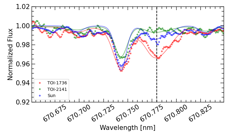
Lithium (Li) is also known to be a sensitive indicator of stellar evolution (e.g., Carlos et al., 2016; Lyubimkov, 2016). To obtain Li abundance, we performed a spectral synthesis analysis using the code iSpec101010https://www.blancocuaresma.com/s/iSpec (Blanco-Cuaresma et al., 2014; Blanco-Cuaresma, 2019) and the radiative transfer code MOOG(Sneden, 1973; Sneden et al., 2012), where we use the lines in the spectral range around Li from Meléndez et al. (2012). Figure 8 illustrates our results, where we show the SOPHIE spectra and the best-fit synthetic models for TOI-1736 and TOI-2141, and also for a solar spectrum obtained from observations of the Moon. We calculated a Li abundance for the solar spectrum of , which is consistent with the expected value for the Sun. For TOI-2141, our results are compatible with a null value, giving an upper limit of A(Li). For TOI-1736, we obtained an abundance of . Using the relationship between A(Li) and age from Carlos et al. (2019) we obtained an age of Gyr for TOI-1736.
All the different age determinations for both systems are presented in Table 5. There is general agreement between the ages of TOI-1736, which are in the range of 4-6 Gyr. For TOI-2141, both the chemical and evolutionary ages agree around 7.5 Gyr, which is consistent with the absence of Li, but the activity-derived age appears younger. For a final determination of the ages of both stars, we adopted the average values, where we added Tayar et al. (2022)’s model uncertainties in quadrature to the measured errors, as in Section 3.5, giving an age of Gyr for TOI-1736 and Gyr for TOI-2141.
| Parameter | TOI-1736 | TOI-2141 |
|---|---|---|
| ¡Age¿ [Chem.; Gyr] | ||
| Age [Iso; Gyr] | ||
| Age [Li; Gyr] | ||
| Age [; Gyr] | ||
| Age model error [Gyr] aaaaadditional error due to systematic differences in stellar evolution models from Tayar et al. (2022)’s method. |
4 Detection and characterization of the planetary systems
4.1 Analysis of TESS photometry data
To further characterize the transits detected by TESS, we analyzed the PDCSAP flux data by applying the methods described in Martioli et al. (2021), where we fit a transit model plus a baseline polynomial in selected windows around each transit in such a way that the window size is twice the duration of the transit and with a minimum of 300 data points. We selected windows for a total of 19 transits of TOI-1736 b and four transits of TOI-2141 b. Our transit model is calculated using the BATMAN toolkit (Kreidberg, 2015) and the posterior distribution of transit parameters is sampled using a Bayesian Monte Carlo Markov Chain (MCMC) framework with the package emcee (Foreman-Mackey et al., 2013). We use uninformative priors for the transit parameters, as presented in Table 12 of Appendix D, with initial values given by those reported in the TESS DVRs and assuming circular orbits.
We divided the TESS light curve by the best-fit transit model and binned the data by the weighted average with bin sizes of 0.1 d to fit a baseline flux using Gaussian processes (GP) regression with a quasi-periodic (QP) kernel as in Martioli et al. (2022). This kernel was chosen to detect a possible variability modulated by the star’s rotation period. The priors of the GP parameters are listed in Table 12 and the posteriors are listed in Table 13. We opted to fix the smoothing factor and decay time values at 0.1 and 10 days, respectively, as altering these values does not impact the other parameters. Unfortunately, the periodicities obtained in our analysis are not well constrained, and their values change significantly depending on the initial guess adopted for our GP model. The low level of intrinsic photometric variability in both targets, coupled with the rotation periods expected from stellar activity (16 – 32 days) being closely aligned with the TESS sector duration, strongly biases the detection of periodicity. This bias is primarily due to systematic variations that occur during TESS observations, particularly near the edges of each sector, where the amplitude of these variations is greater. While there may be some intrinsic stellar variability captured by TESS photometry, the GP model obtained here may account for both systematic and intrinsic stellar phenomena in unknown proportions.
Since the periodic kernel is not essential, the primary purpose of employing the GP in this analysis is for detrending. To ensure that the choice of GP does not impact the planet parameters, we conducted experiments using both a squared exponential (SE) kernel and a model without GP. The posterior distributions of key planet parameters (, , , and ) are consistent within 1-sigma for all three choices of baseline model. The results of our best-fit transit models and GP analysis using a QP kernel are illustrated in Figures 1 and 2.
4.2 Radial velocities
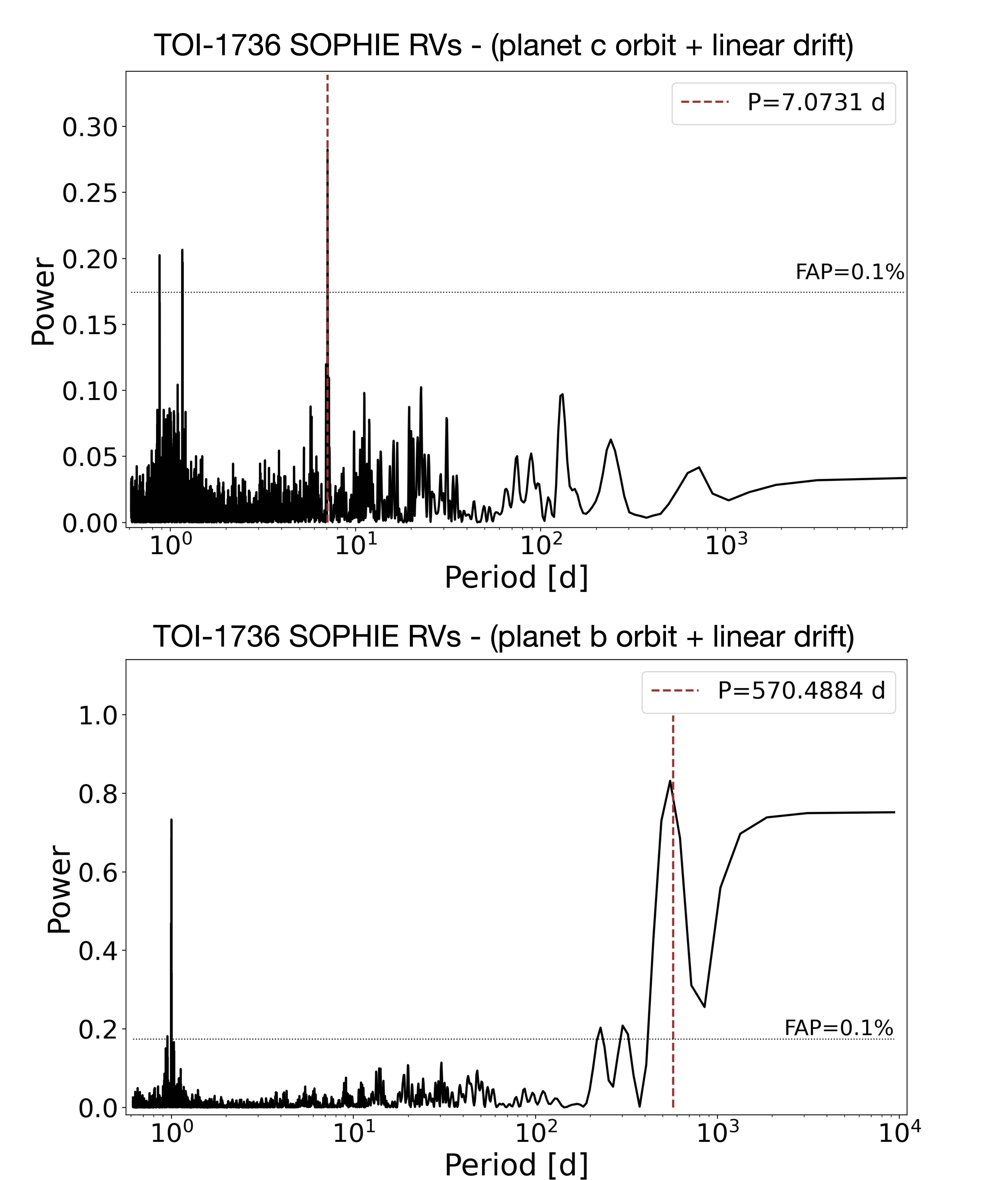
The TOI-1736 RVs have a median value of -25408.95 m s-1 with an rms of 158 m s-1 and a median individual error of 2 m s-1. These RVs present a clear signal with an amplitude of hundreds of m s-1, as can be seen in Figure 13. An initial analysis of the generalized Lomb-Scargle (GLS) periodogram (Zechmeister & Kürster, 2009) of this data show that there is a dominating signal with periodicity around 570 d and a long-term linear trend was also detected by visual inspection. To detect the TESS candidate planet, TOI-1736.01, at a period of 7.073 d, we fit the SOPHIE RV data using the online tool Data & Analysis Center for Exoplanets (DACE121212https://dace.unige.ch), where we adopted a two-planet Keplerian model plus a linear trend. As illustrated in Figure 9, the GLS of the RVs after subtracting the linear trend and each planet’s orbit shows a strong peak at 7.0731 d and 570.07 d for the inner and outer planet, respectively. The former agrees well with the periodicity of the transits detected by TESS, showing the RV detection of the inner planet candidate, TOI-1736 b, and an outer giant planet, TOI-1736 c. Moreover, this confirms that transits detected by TESS occur in the primary star, as the dominant flux in the SOPHIE spectra comes from the primary and not from the K3 dwarf companion. As a way to test if the SOPHIE spectra are contaminated by the flux from the companion, we performed a CCF analysis using a K0, K5, or M0 masks, which should favor the detection of spectral lines of the cooler star. Those tests resulted in slightly noisier CCF with parameters in agreement as when using the G2 mask, showing that indeed, the flux contribution of the companion to the RV measurements in the SOPHIE spectra is negligible.
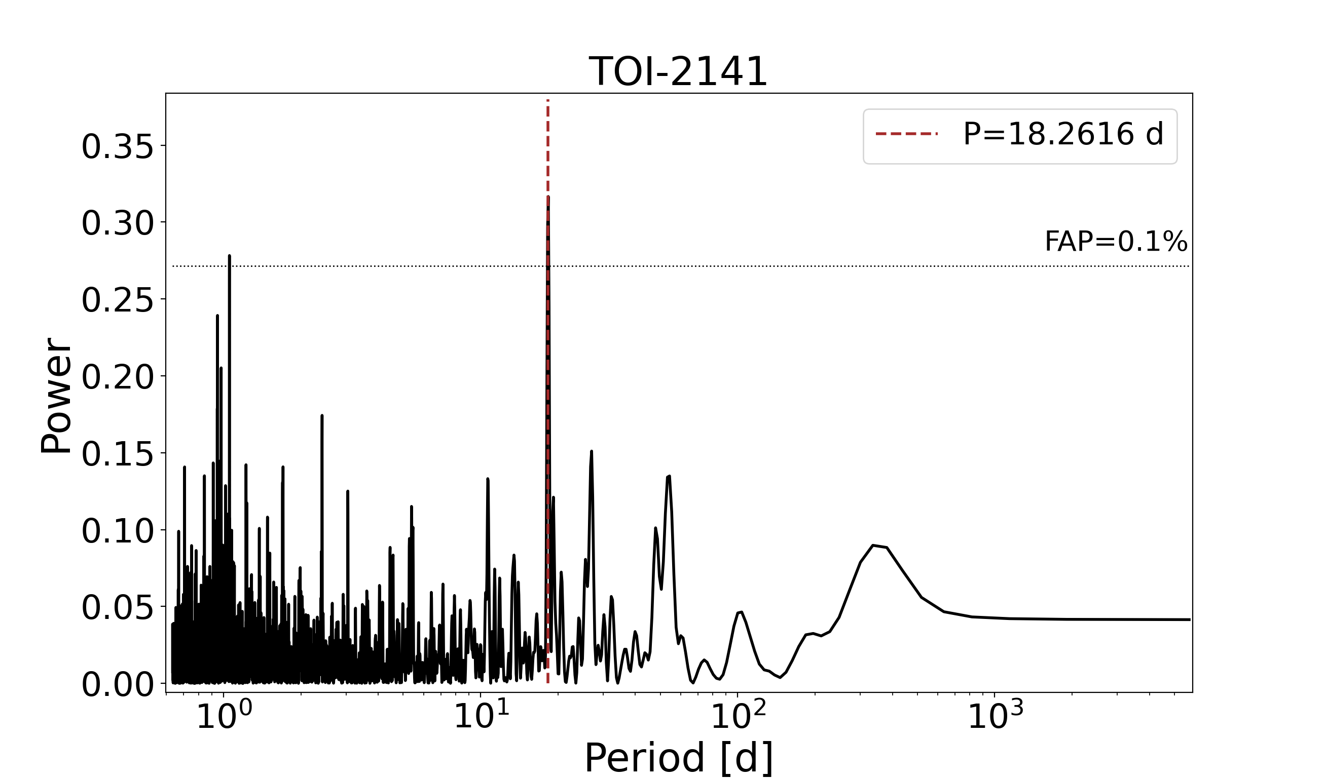
The TOI-2141 RVs have a median value of -19860.8 m s-1 with an rms of 7 m s-1 and a median individual error of 2.4 m s-1. The RVs of this object do not appear to have any long-term trends or variability. Figure 10 shows the GLS periodogram for this data, which shows the highest peak at a period of 18.259 d, again in agreement with the periodicity of the transits detected by TESS. This shows the detection of the planet candidate TOI-2141 b in our SOPHIE data. In the following sections, we present an analysis to characterize these two planetary systems.
For both systems, we found that there is no correlation between the RVs and the four stellar activity indicators: FWHM, BIS, Hα, and S-index. Therefore, the signals detected in RV are probably due to Doppler shift and not to scenarios that imply changes in the line profile, for example, blended binaries. We have also inspected possible correlations between the RV residuals (after subtracting the fit models) and activity indicators. Only BIS shows a slight correlation of 0.29 and 0.15 for TOI-1736 and TOI-2141, respectively. We tried to de-correlate the RVs as in Boisse et al. (2009), but this did not have a significant impact on the values of the fit parameters, so we preferred to keep the final analysis without applying this correction. In the Appendix C we show the time series of each activity indicator, an analysis of the GLS periodogram, and its correlations with the RV data.
4.3 Joint analysis of RVs and photometry to characterize the planets
To obtain the physical parameters of the planets, we perform a joint analysis of the photometry and RV data sets as in Martioli et al. (2022). We adopt the priors listed in Table 12 and the initial values are those obtained by the analysis performed on the SOPHIE RVs and TESS photometry data independently.
We first fit the RV orbits and transit models jointly using the scipy.optimize.leastsq optimization tool. Then, we use the same tool to fit the RV jitter, which is a term quadratically added to the RV errors. Finally, we explore the full range covered by the priors with a Bayesian MCMC that uses 50 random walkers, with 10000 iterations, discarding the first 3000 burn-in samples. The posterior distributions of sampled parameters are illustrated in Appendix D and the resulting best-fit parameters, obtained from the mode of the posterior and 1 uncertainties (34% on each side of the central value) are given in Table 6. Some parameters converged to values close to the edge of their physical domains. For example, it happened for the orbital inclination ( deg) and the linear limb-darkening coefficient () for both transiting planets, TOI-1736 b and TOI-2141 b. We also adopted circular orbits (, deg) for both inner planets, as noncircular solutions resulted in higher values of the Bayesian Information Criterion (BIC), suggesting that our data cannot constrain the low values of the eccentricities of these planets.
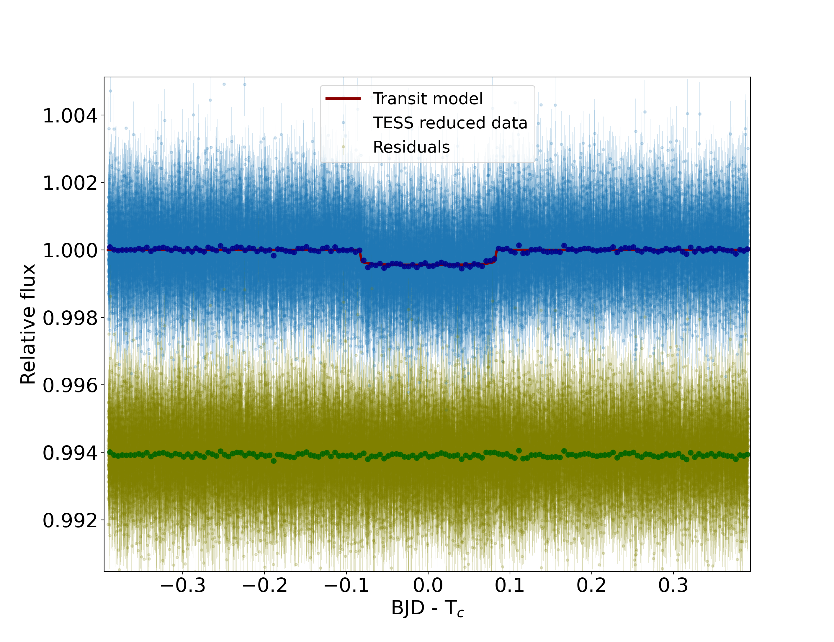
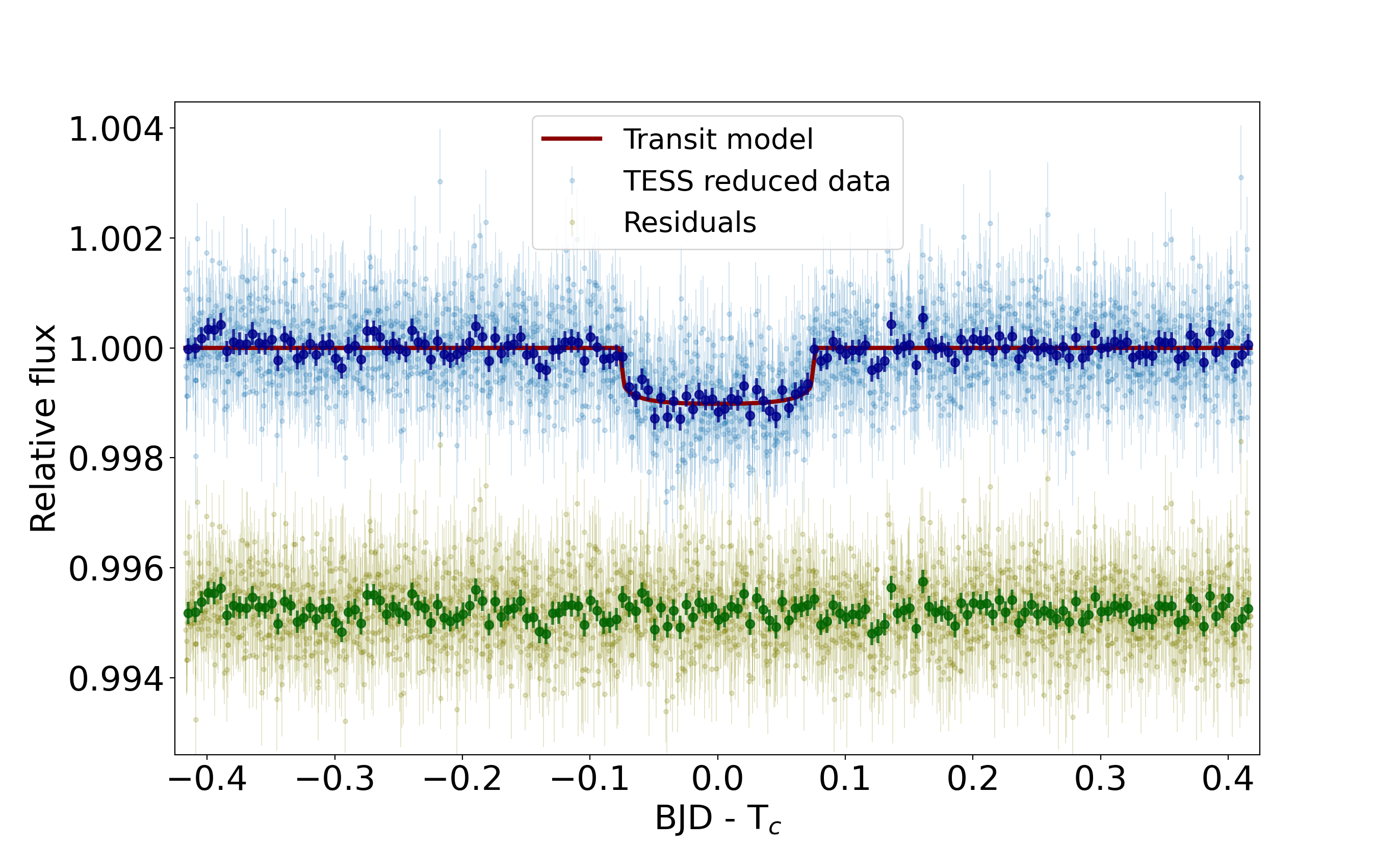
Figures 12 and 11 illustrate the TESS photometry data for all transits detected by TESS and the best-fit transit models obtained by our joint analysis. Figure 13 and 14 illustrate the TOI-1736 RV data and the best-fit models that include the orbit of the two planets, TOI-1736 b and TOI-1736 c, and the linear trend. Figures 15 and 16 illustrate the RV data and best-fit model for TOI-2141.


| Parameter | TOI-1736 b | TOI-1736 c | TOI-2141 b |
|---|---|---|---|
| time of conjunction, (BJD) | |||
| orbital period, (d) | |||
| eccentricity, | |||
| argument of periastron, (deg) | 90 | 90 | |
| normalized semimajor axis, | |||
| semimajor axis, aaaasemi-major axis derived from the fit period and Kepler’s law. (au) | |||
| orbital inclination, (deg) | |||
| transit duration, (h) | |||
| impact parameter, | |||
| planet-to-star radius ratio, | |||
| planet radius, (RJup) | |||
| planet radius, (RNep) | |||
| planet radius, (R♁) | |||
| velocity semi-amplitude, (m s-1) | |||
| planet mass, (MJup) | |||
| planet mass, (MNep) | |||
| planet mass, (M♁) | |||
| planet min. mass, (MJup) | |||
| planet density, (g cm-3) | |||
| equilibrium temperature, bbbbassuming a uniform heat redistribution and an arbitrary geometric albedo of 0.1. (K) | |||
| linear limb dark. coef., | |||
| quadratic limb dark. coef., | |||
| RV linear trend, (m s-1 d-1) | 0 | ||
| RV jitter, (m s-1) | |||
| RMS of RV residuals (m s-1) | 5.0 | 5.0 | 6.5 |
| RMS of flux residuals (ppm) | 941 | 630 | |
5 GAIA astrometry to constrain the mass of TOI-1736 c
The expected astrometric signal due to the orbit of the star TOI-1736 around the center of mass of the system can be estimated by the following equation:
| (1) |
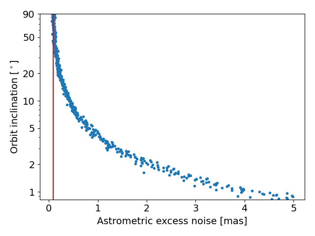
where is the parallax in milli-arcseconds, is the semi-major axis of the planet’s orbit in au, is the planet’s mass and is the stellar mass. For TOI-1736 c, we estimate mas. Here, we use the method Gaia Astrometric noise Simulation To derive Orbit iNclination (GASTON; Kiefer, 2019; Kiefer et al., 2019) to constrain, from GAIA DR3 (Gaia Collaboration et al., 2021) astrometric excess noise and RV-derived orbital parameters, the orbital inclination and true mass of TOI-1736 c. The GAIA DR3 astrometric excess noise of TOI-1736 is mas. Figure 17 shows the results of our GASTON simulations of astrometric excess noise as a function of the orbital inclination, assuming the RV orbit of TOI-1736 c. We obtained an orbital inclination of deg, which gives a semi-major axis of the star photocenter of mas.
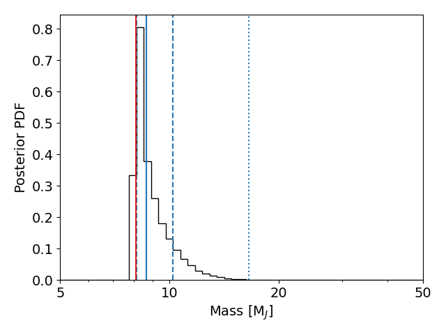
These results show that the orbit of the TOI-1736 c seems to be tilted with respect to the inner planet, but is not inconsistent, within , with a coplanar orientation. Assuming coplanarity, we computed the prospective transit epochs for TOI-1736 c; however, none of the predicted events align with TESS observations. Finally, we derived the mass of TOI-1736 c by considering our measurements of combined with the astrometric constraint. Figure 18 shows the posterior distribution for the mass of TOI-1736 c, where we obtained at with a maximum value of MJup at .
6 Discussions
The SOPHIE RV data show periodic variations at the same period as the transits detected by TESS, where the orbital fit gives a semi-amplitude of m s-1 for TOI-1736 b and m s-1 for TOI-2141 b. The TOI-1736 RVs also revealed an outer giant planet TOI-1736 c with an RV semi-amplitude of m s-1, in addition to a long term linear trend of m s-1 d-1. This trend could be due to the perturbation caused by the orbital motion of an outer planetary or stellar companion. We note that this deviation could be caused by the K-dwarf stellar companion that we detected with photometry, although we did not detect its signature in GAIA’s excess astrometric noise. Current SOPHIE data are not sufficient to distinguish at what periodicity and amplitude this variability occurs. Therefore, we have not yet inferred any characterization for this possible companion, and we will continue to monitor this star in the coming years to discover the nature of this signal in future work.
The inner planets, TOI-1736 b and TOI-2141 b, with radii of R♁ and R♁ and masses of M♁ and M♁ have similar mean densities of g cm-3 and g cm-3, respectively. The giant planet TOI-1736 c has a mass of MJup and orbits the star with a period of d and an orbital eccentricity of . With a semi-major axis of au, this giant resides in a temperate orbit around the star, which is in the habitable zone of that star as detailed in Section 6.1. TOI-1736 is therefore similar to the system HD 137496 (K2-364) (Azevedo Silva et al., 2022), which is also a solar analog hosting a hot, dense inner planet and an outer giant with about the same mass as TOI-1736 c and with similar orbital properties. Both are nearby and bright systems, making them interesting cases to study the evolution of planetary systems around solar analogs and, in particular, studying the occupation of their habitable zones by giant planets.
6.1 The exoplanets’ radiation environment
We consider the best-fit parameters from our analysis to calculate the habitable zone for these solar analogs, using the equations and data from Kopparapu et al. (2014). We obtained an optimistic lower limit (recent Venus) at 0.87 au for TOI-1736 and 0.71 au for TOI-2141, and an upper limit (early Mars) at 2.05 au for TOI-1736 and 1.68 au for TOI-2141. The runaway greenhouse limits ( M♁) ranges between 1.10 au and 1.94 au for TOI-1736, and between 0.90 au and 1.59 au for TOI-2141.
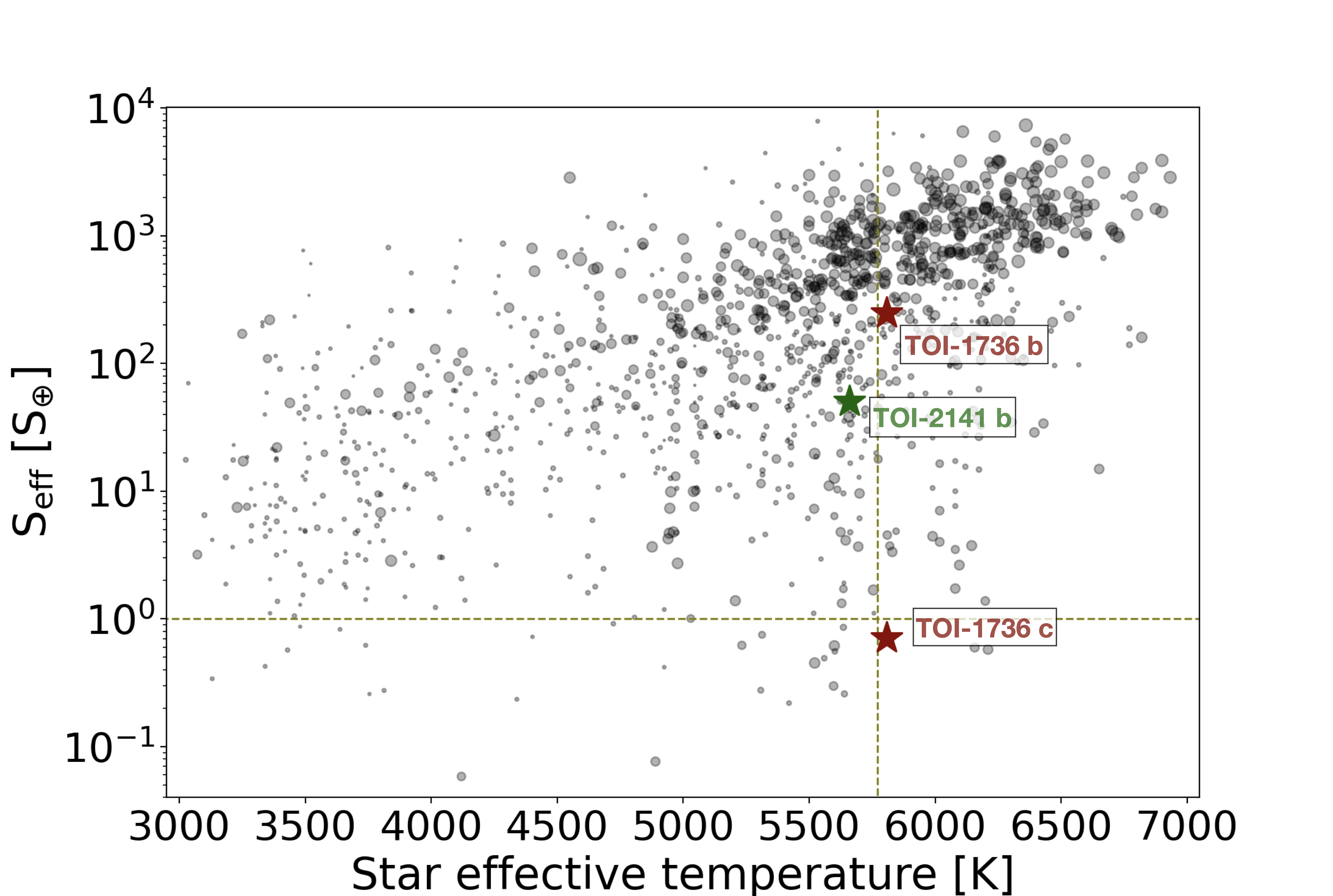
To estimate the level of radiation that each planet receives from its host star, we calculate the effective insolation flux relative to the flux incident on Earth as , where is the star luminosity in solar units and is the semi-major axis of the planet’s orbit in au. Figure 19 shows the insolation for exoplanets as a function of star effective temperature. TOI-1736 b and TOI-2141 b receive an insolation of and , respectively, showing that these planets reside in a hot environment. We estimate the equilibrium temperature for the planets as in Heng & Demory (2013), assuming a uniform heat redistribution and an arbitrary geometric albedo of 0.1, which gives K and K for TOI-1736 b and TOI-2141 b, respectively.
On the other hand, TOI-1736 c resides at a larger distance from the star, in an eccentric orbit with , and a semi-minor axis of au and a semi-major axis of au. At these distances, TOI-1736 c receives an insolation of and for which we estimate an equilibrium temperature of K and K, respectively. This planet resides within the conservative habitable zone around the star.
6.2 Mass-radius relation for the inner planets
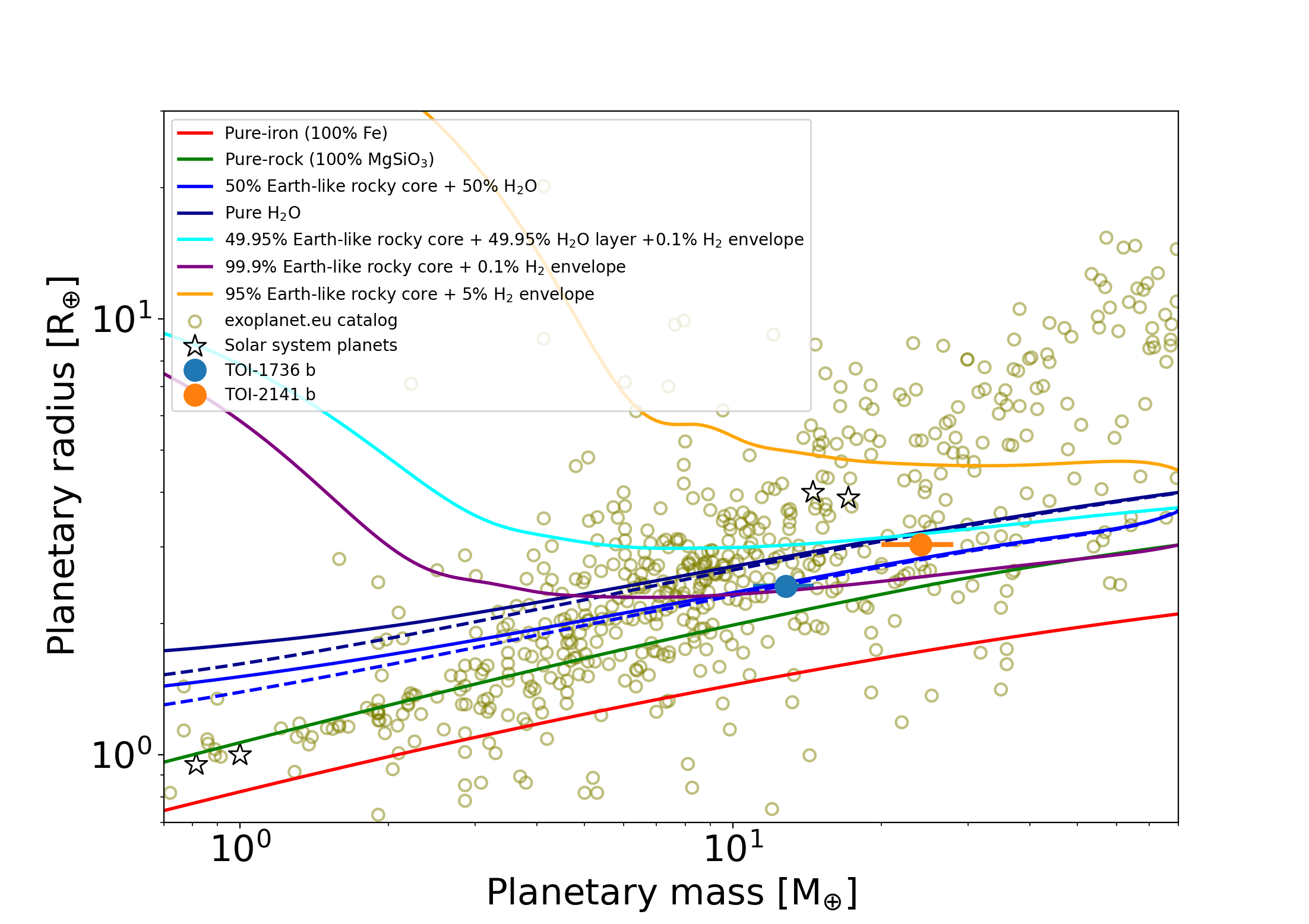
From mass and radius measurements of the transiting planets TOI-1736 b and TOI 2141 b, we derive their mean densities of g cm-3 and g cm-3, respectively, showing that these sub-Neptune sized planets have densities similar to the rocky planets of the Solar System. To explore further the possible chemical composition and structure of these planets we inspect the mass-radius (M-R) diagram illustrated in Figure 20, which shows the exoplanet data from exoplanets.eu, the data from the two hot sub-Neptunes studied here, and a set of models from Zeng et al. (2019), for comparison. The M-R location of TOI-1736 b matches two models: (1) a 50% Earth-like rocky core plus a 50% H2O layer; (2) an almost pure Earth-like rocky core with a thin 0.1% H2 envelop. Therefore, this planet probably has a large dense rocky core surrounded by either a thick water-rich atmosphere or a thin H2 atmosphere. TOI-2141 b is compatible with three scenarios: (1) a 50% Earth-like rocky core with a 50% H2O layer; (2) a 49.95% Earth-like rocky core + 49.95% H2O layer and a thin 0.1% H2 envelop; and (3) a pure H2O. Thus, TOI-2141 b is likely a water-rich planet. A further investigation of the internal structure of these planets can be done by including simulations constrained by the star metallicity and abundances of volatiles, which is out of the scope of this paper.
7 Conclusions
We reported the discovery of two new planetary systems around the solar analogs TOI-1736 and TOI-2141. We monitored these systems spectroscopically with the SOPHIE instrument at OHP to obtain high-precision RV time series. These data show periodic variations at the same period as the transiting candidates detected by TESS, establishing the planetary nature of the sub-Neptunes TOI-1736 b and TOI-2141 b. Our RV data also revealed an outer giant planet in the TOI-1736 system, in addition to a long-term linear trend. This drift could be due to an additional companion that will be investigated further in future observations.
We characterized the two host stars by analyzing their high-resolution spectra combined with photometry and high-contrast imaging data. We found that TOI-1736 likely has a K3 dwarf stellar companion, which is evidenced both by the power spectrum of the speckle imaging data at 832 nm and by an infrared excess in the SED. The presence of this companion has an important impact on the determination of the star’s radius, which affects the derivation of the planet’s radius and other physical properties of the system. The flux of this possible companion has a negligible contribution to our high-resolution SOPHIE spectra.
We obtained the stellar parameters from several methods, including a SED fit analysis of the photometry data, a spectral analysis of the high-resolution SOPHIE and TRES spectra, and a differential analysis of the SOPHIE spectra using a solar spectrum from observations of the Moon as a reference. The latter provides the most accurate stellar parameters, which also improves the determination of the physical parameters of the planets. This shows the importance of studying planetary systems around solar analogs, where the solar spectrum can benchmark measurements of stellar properties and therefore provide more accurate values. We also determined elemental abundances for several species, including refractory elements (Fe, Mg, and Si) that provide constraints for the planet’s interior structure models. We found that both systems exhibit low levels of stellar activity from their , which are consistent with their non-variable time series of activity indices, and with the mature ages of about 5 Gyr for TOI-1736 and 7 Gyr for TOI-2141, found from chemical clocks and evolutionary analyses. The inferred radii and stellar masses for these two stars have values that differ by about of solar values, showing that they are indeed solar analogs, but not solar twins.
Therefore, these two new systems represent perspectives on how planetary systems can form and evolve around solar analogs. On the one hand, we have TOI-2141, an evolved star that hosts a warm sub-Neptune with a likely dense rocky core and a possible thick, water-rich envelope. On the other hand, we have TOI-1736, a hierarchical star system with a solar analog that hosts a hot, dense sub-Neptune and an outer giant planet in an eccentric orbit in the habitable zone.
Acknowledgements.
E.M. acknowledges funding from Fundação de Amparo à Pesquisa do Estado de Minas Gerais (FAPEMIG) under project number APQ-02493-22 and research productivity grant (PQ) number 309829/2022-4 awarded by the National Council for Scientific and Technological Development (CNPq), Brazil. We thank the Observatoire de Haute-Provence (CNRS) staff for their support. This work was supported by the “Programme National de Planétologie” (PNP) of CNRS/INSU and CNES. This paper includes data collected with the TESS mission, obtained from the MAST data archive at the Space Telescope Science Institute (STScI). Funding for the TESS mission is provided by NASA’s Science Mission Directorate. We acknowledge the use of public TESS data from pipelines at the TESS Science Office and at the TESS Science Processing Operations Center. Resources supporting this work were provided by the NASA High-End Computing (HEC) Program through the NASA Advanced Supercomputing (NAS) Division at Ames Research Center for the production of the SPOC data products. This publication makes use of The Data & Analysis Center for Exoplanets (DACE), which is a facility based at the University of Geneva (CH) dedicated to extrasolar planets data visualization, exchange, and analysis. DACE is a platform of the Swiss National Centre of Competence in Research (NCCR) PlanetS, federating the Swiss expertise in Exoplanet research. The DACE platform is available at https://dace.unige.ch. We acknowledge funding from the French ANR under contract number ANR18CE310019 (SPlaSH). X.D. and T.F. acknoweldge support by the French National Research Agency in the framework of the Investissement d’Avenir program (ANR-15-IDEX-02), through the funding of the ”Origin of Life” project of the Grenoble-Alpes University. This work was supported by FCT - Fundação para a Ciência e a Tecnologia through national funds and by FEDER through COMPETE2020 - Programa Operacional Competitividade e Internacionalizacão by these grants: UID/FIS/04434/2019, UIDB/04434/2020, UIDP/04434/2020, PTDC/FIS-AST/32113/2017 & POCI-01-0145-FEDER- 032113, PTDC/FIS-AST/28953/2017 & POCI-01-0145-FEDER-028953, PTDC/FIS-AST/28987/2017 & POCI-01-0145-FEDER-028987. NCS further acknowledges funding by the European Union (ERC, FIERCE, 101052347). Views and opinions expressed are however those of the author(s) only and do not necessarily reflect those of the European Union or the European Research Council. Neither the European Union nor the granting authority can be held responsible for them. This work makes use of observations from the LCOGT network. Part of the LCOGT telescope time was granted by NOIRLab through the Mid-Scale Innovations Program (MSIP). MSIP is funded by NSF. KAC acknowledges support from the TESS mission via subaward s3449 from MIT. S.D. is funded by the UK Science and Technology Facilities Council (grant number ST/V004735/1). S.G.S acknowledges the support from FCT through the contract nr.CEECIND/00826/2018 and POPH/FSE (EC).References
- Adibekyan et al. (2021) Adibekyan, V., Dorn, C., Sousa, S. G., et al. 2021, Science, 374, 330
- Azevedo Silva et al. (2022) Azevedo Silva, T., Demangeon, O. D. S., Barros, S. C. C., et al. 2022, A&A, 657, A68
- Bedell et al. (2014) Bedell, M., Meléndez, J., Bean, J. L., et al. 2014, ApJ, 795, 23
- Blanco-Cuaresma (2019) Blanco-Cuaresma, S. 2019, MNRAS, 486, 2075
- Blanco-Cuaresma et al. (2014) Blanco-Cuaresma, S., Soubiran, C., Heiter, U., & Jofré, P. 2014, A&A, 569, A111
- Boisse et al. (2010) Boisse, I., Eggenberger, A., Santos, N. C., et al. 2010, A&A, 523, A88
- Boisse et al. (2009) Boisse, I., Moutou, C., Vidal-Madjar, A., et al. 2009, A&A, 495, 959
- Bouchy et al. (2013) Bouchy, F., Díaz, R. F., Hébrard, G., et al. 2013, A&A, 549, A49
- Bouchy et al. (2009) Bouchy, F., Hébrard, G., Udry, S., et al. 2009, A&A, 505, 853
- Brown et al. (2013) Brown, T. M., Baliber, N., Bianco, F. B., et al. 2013, PASP, 125, 1031
- Buchhave et al. (2010) Buchhave, L. A., Bakos, G. Á., Hartman, J. D., et al. 2010, ApJ, 720, 1118
- Buchhave et al. (2012) Buchhave, L. A., Latham, D., Johansen, A., et al. 2012, Nature, 486, 375
- Carlos et al. (2019) Carlos, M., Meléndez, J., Spina, L., et al. 2019, MNRAS, 485, 4052
- Carlos et al. (2016) Carlos, M., Nissen, P. E., & Meléndez, J. 2016, A&A, 587, A100
- Castelli & Kurucz (2003) Castelli, F. & Kurucz, R. L. 2003, in Modelling of Stellar Atmospheres, ed. N. Piskunov, W. W. Weiss, & D. F. Gray, Vol. 210, A20
- Ciardi et al. (2015) Ciardi, D. R., Beichman, C. A., Horch, E. P., & Howell, S. B. 2015, ApJ, 805, 16
- Cincunegui et al. (2007) Cincunegui, C., Díaz, R. F., & Mauas, P. J. D. 2007, A&A, 469, 309
- Collins (2019) Collins, K. 2019, in American Astronomical Society Meeting Abstracts, Vol. 233, American Astronomical Society Meeting Abstracts #233, 140.05
- Collins et al. (2017) Collins, K. A., Kielkopf, J. F., Stassun, K. G., & Hessman, F. V. 2017, AJ, 153, 77
- Courcol et al. (2015) Courcol, B., Bouchy, F., Pepe, F., et al. 2015, A&A, 581, A38
- Cutri et al. (2003) Cutri, R. M., Skrutskie, M. F., van Dyk, S., et al. 2003, VizieR Online Data Catalog, II/246
- Czesla et al. (2019) Czesla, S., Schröter, S., Schneider, C. P., et al. 2019, PyA: Python astronomy-related packages
- da Silva et al. (2012) da Silva, R., Porto de Mello, G. F., Milone, A. C., et al. 2012, A&A, 542, A84
- Delgado Mena et al. (2019) Delgado Mena, E., Moya, A., Adibekyan, V., et al. 2019, A&A, 624, A78
- Demarque et al. (2004) Demarque, P., Woo, J.-H., Kim, Y.-C., & Yi, S. K. 2004, ApJS, 155, 667
- Donati et al. (2020) Donati, J. F., Kouach, D., Moutou, C., et al. 2020, MNRAS, 498, 5684
- Dorn et al. (2015) Dorn, C., Khan, A., Heng, K., et al. 2015, A&A, 577, A83
- Duncan et al. (1991) Duncan, D. K., Vaughan, A. H., Wilson, O. C., et al. 1991, ApJS, 76, 383
- Egeland et al. (2017) Egeland, R., Soon, W., Baliunas, S., et al. 2017, ApJ, 835, 25
- Fűrész et al. (2008) Fűrész, G., Szentgyorgyi, A. H., & Meibom, S. 2008, in Precision Spectroscopy in Astrophysics, ed. N. C. Santos, L. Pasquini, A. C. M. Correia, & M. Romaniello, 287–290
- Foreman-Mackey et al. (2013) Foreman-Mackey, D., Hogg, D. W., Lang, D., & Goodman, J. 2013, PASP, 125, 306
- Gaia Collaboration (2020) Gaia Collaboration. 2020, VizieR Online Data Catalog, I/350
- Gaia Collaboration et al. (2021) Gaia Collaboration, Brown, A. G. A., Vallenari, A., et al. 2021, A&A, 649, A1
- Grieves et al. (2018) Grieves, N., Ge, J., Thomas, N., et al. 2018, MNRAS, 481, 3244
- Guerrero et al. (2021) Guerrero, N. M., Seager, S., Huang, C. X., et al. 2021, ApJS, 254, 39
- Hauschildt et al. (1999) Hauschildt, P. H., Allard, F., & Baron, E. 1999, ApJ, 512, 377
- Hébrard et al. (2008) Hébrard, G., Bouchy, F., Pont, F., et al. 2008, A&A, 488, 763
- Hébrard et al. (2020) Hébrard, G., Díaz, R. F., Correia, A. C. M., et al. 2020, A&A, 640, A32
- Heidari et al. (2022) Heidari, N., Boisse, I., Orell-Miquel, J., et al. 2022, A&A, 658, A176
- Heng & Demory (2013) Heng, K. & Demory, B.-O. 2013, ApJ, 777, 100
- Howell et al. (2011) Howell, S. B., Everett, M. E., Sherry, W., Horch, E., & Ciardi, D. R. 2011, AJ, 142, 19
- Jenkins (2002) Jenkins, J. M. 2002, ApJ, 575, 493
- Jenkins et al. (2010) Jenkins, J. M., Chandrasekaran, H., McCauliff, S. D., et al. 2010, in Society of Photo-Optical Instrumentation Engineers (SPIE) Conference Series, Vol. 7740, Software and Cyberinfrastructure for Astronomy, ed. N. M. Radziwill & A. Bridger, 77400D
- Jenkins et al. (2020) Jenkins, J. M., Tenenbaum, P., Seader, S., et al. 2020, Kepler Data Processing Handbook: Transiting Planet Search, Kepler Science Document KSCI-19081-003, id. 9. Edited by Jon M. Jenkins.
- Jenkins et al. (2016) Jenkins, J. M., Twicken, J. D., McCauliff, S., et al. 2016, in Proc. SPIE, Vol. 9913, Software and Cyberinfrastructure for Astronomy IV, 99133E
- Kiefer (2019) Kiefer, F. 2019, A&A, 632, L9
- Kiefer et al. (2019) Kiefer, F., Hébrard, G., Sahlmann, J., et al. 2019, A&A, 631, A125
- König et al. (2022) König, P. C., Damasso, M., Hébrard, G., et al. 2022, A&A, 666, A183
- Kopparapu et al. (2014) Kopparapu, R. K., Ramirez, R. M., SchottelKotte, J., et al. 2014, ApJ, 787, L29
- Kreidberg (2015) Kreidberg, L. 2015, PASP, 127, 1161
- Kurucz (1992) Kurucz, R. L. 1992, in The Stellar Populations of Galaxies, ed. B. Barbuy & A. Renzini, Vol. 149, 225
- Lallement et al. (2014) Lallement, R., Vergely, J. L., Valette, B., et al. 2014, A&A, 561, A91
- Li et al. (2019) Li, J., Tenenbaum, P., Twicken, J. D., et al. 2019, PASP, 131, 024506
- Lorenzo-Oliveira et al. (2018) Lorenzo-Oliveira, D., Freitas, F. C., Meléndez, J., et al. 2018, A&A, 619, A73
- Lorenzo-Oliveira et al. (2016) Lorenzo-Oliveira, D., Porto de Mello, G. F., & Schiavon, R. P. 2016, A&A, 594, L3
- Lyubimkov (2016) Lyubimkov, L. S. 2016, Astrophysics, 59, 411
- MacDougall et al. (2023) MacDougall, M. G., Petigura, E. A., Gilbert, G. J., et al. 2023, arXiv e-prints, arXiv:2306.00251
- Mamajek & Hillenbrand (2008) Mamajek, E. E. & Hillenbrand, L. A. 2008, ApJ, 687, 1264
- Martioli et al. (2021) Martioli, E., Hébrard, G., Correia, A. C. M., Laskar, J., & Lecavelier des Etangs, A. 2021, A&A, 649, A177
- Martioli et al. (2022) Martioli, E., Hébrard, G., Fouqué, P., et al. 2022, A&A, 660, A86
- McCully et al. (2018) McCully, C., Volgenau, N. H., Harbeck, D.-R., et al. 2018, in Society of Photo-Optical Instrumentation Engineers (SPIE) Conference Series, Vol. 10707, Software and Cyberinfrastructure for Astronomy V, ed. J. C. Guzman & J. Ibsen, 107070K
- Meléndez et al. (2012) Meléndez, J., Bergemann, M., Cohen, J. G., et al. 2012, A&A, 543, A29
- Meléndez et al. (2014) Meléndez, J., Ramírez, I., Karakas, A. I., et al. 2014, ApJ, 791, 14
- Mittag et al. (2013) Mittag, M., Schmitt, J. H. M. M., & Schröder, K. P. 2013, A&A, 549, A117
- Moutou et al. (2021) Moutou, C., Almenara, J. M., Hébrard, G., et al. 2021, A&A, 653, A147
- Perruchot et al. (2008) Perruchot, S., Kohler, D., Bouchy, F., et al. 2008, in Society of Photo-Optical Instrumentation Engineers (SPIE) Conference Series, Vol. 7014, Ground-based and Airborne Instrumentation for Astronomy II, ed. I. S. McLean & M. M. Casali, 70140J
- Pollacco et al. (2008) Pollacco, D., Skillen, I., Collier Cameron, A., et al. 2008, MNRAS, 385, 1576
- Queloz et al. (2001) Queloz, D., Henry, G. W., Sivan, J. P., et al. 2001, A&A, 379, 279
- Ramírez et al. (2014) Ramírez, I., Meléndez, J., Bean, J., et al. 2014, A&A, 572, A48
- Ricker et al. (2015) Ricker, G. R., Winn, J. N., Vanderspek, R., et al. 2015, Journal of Astronomical Telescopes, Instruments, and Systems, 1, 014003
- Santos et al. (2004) Santos, N. C., Israelian, G., & Mayor, M. 2004, A&A, 415, 1153
- Santos et al. (2013) Santos, N. C., Sousa, S. G., Mortier, A., et al. 2013, A&A, 556, A150
- Smith et al. (2012) Smith, J. C., Stumpe, M. C., Van Cleve, J. E., et al. 2012, PASP, 124, 1000
- Sneden et al. (2012) Sneden, C., Bean, J., Ivans, I., Lucatello, S., & Sobeck, J. 2012, MOOG: LTE line analysis and spectrum synthesis, Astrophysics Source Code Library, record ascl:1202.009
- Sneden (1973) Sneden, C. A. 1973, PhD thesis, University of Texas, Austin
- Soderblom & King (1998) Soderblom, D. R. & King, J. R. 1998, in Solar Analogs: Characteristics and Optimum Candidates., ed. J. C. Hall, 41
- Sousa et al. (2008) Sousa, S. G., Santos, N. C., Mayor, M., et al. 2008, A&A, 487, 373
- Spina et al. (2018) Spina, L., Meléndez, J., Casey, A. R., Karakas, A. I., & Tucci-Maia, M. 2018, ApJ, 863, 179
- Stassun et al. (2017) Stassun, K. G., Collins, K. A., & Gaudi, B. S. 2017, AJ, 153, 136
- Stassun et al. (2018) Stassun, K. G., Corsaro, E., Pepper, J. A., & Gaudi, B. S. 2018, AJ, 155, 22
- Stassun & Torres (2016) Stassun, K. G. & Torres, G. 2016, AJ, 152, 180
- Stassun & Torres (2021) Stassun, K. G. & Torres, G. 2021, ApJ, 907, L33
- Stumpe et al. (2014) Stumpe, M. C., Smith, J. C., Catanzarite, J. H., et al. 2014, PASP, 126, 100
- Stumpe et al. (2012) Stumpe, M. C., Smith, J. C., Van Cleve, J. E., et al. 2012, PASP, 124, 985
- Tayar et al. (2022) Tayar, J., Claytor, Z. R., Huber, D., & van Saders, J. 2022, ApJ, 927, 31
- Torres et al. (2010) Torres, G., Andersen, J., & Giménez, A. 2010, A&A Rev., 18, 67
- Tucci Maia et al. (2015) Tucci Maia, M., Meléndez, J., Castro, M., et al. 2015, A&A, 576, L10
- Twicken et al. (2018) Twicken, J. D., Catanzarite, J. H., Clarke, B. D., et al. 2018, PASP, 130, 064502
- Wilson (1968) Wilson, O. C. 1968, ApJ, 153, 221
- Wright et al. (2010) Wright, E. L., Eisenhardt, P. R. M., Mainzer, A. K., et al. 2010, AJ, 140, 1868
- Yana Galarza et al. (2021) Yana Galarza, J., López-Valdivia, R., Lorenzo-Oliveira, D., et al. 2021, MNRAS, 504, 1873
- Yana Galarza et al. (2019) Yana Galarza, J., Meléndez, J., Lorenzo-Oliveira, D., et al. 2019, MNRAS, 490, L86
- Yi et al. (2001) Yi, S., Demarque, P., Kim, Y.-C., et al. 2001, ApJS, 136, 417
- Zechmeister & Kürster (2009) Zechmeister, M. & Kürster, M. 2009, A&A, 496, 577
- Zeng et al. (2019) Zeng, L., Jacobsen, S. B., Sasselov, D. D., et al. 2019, Proceedings of the National Academy of Science, 116, 9723
Appendix A SOPHIE RVs and spectroscopic quantities
This appendix presents a compilation of all quantities derived from the SOPHIE spectra. Tables LABEL:tab:sophiervstoi1736 and LABEL:tab:sophiervstoi2141 show these quantities obtained for the spectra of TOI-1736 and TOI-2141, respectively.
| Obs | Time | RV | BERV | Exptime | S/N | FWHM | Bis | SMW | Hα | |||||
|---|---|---|---|---|---|---|---|---|---|---|---|---|---|---|
| index | BJD | km s-1 | km s-1 | km s-1 | s | @649 nm | km s-1 | km s-1 | km s-1 | km s-1 | ||||
| 1 | 2459081.61496 | -25.2590 | 0.0025 | 18.9856 | 285 | 55 | 8.207 | 0.022 | 0.001 | 0.013 | 0.136 | 0.036 | 0.2481 | 0.0023 |
| 2 | 2459084.64339 | -25.2680 | 0.0026 | 19.0918 | 742 | 54 | 8.188 | 0.022 | -0.021 | 0.010 | 0.161 | 0.038 | 0.2405 | 0.0016 |
| 3 | 2459085.62038 | -25.2669 | 0.0026 | 19.1373 | 580 | 55 | 8.184 | 0.022 | -0.013 | 0.005 | 0.158 | 0.038 | 0.2411 | 0.0018 |
| 4 | 2459106.60980 | -25.2690 | 0.0025 | 18.5376 | 297 | 56 | 8.203 | 0.022 | -0.023 | 0.012 | 0.119 | 0.037 | 0.2425 | 0.0018 |
| 5 | 2459107.65934 | -25.2704 | 0.0025 | 18.4075 | 402 | 57 | 8.175 | 0.022 | -0.051 | 0.009 | 0.121 | 0.036 | 0.2484 | 0.0018 |
| 6 | 2459113.61605 | -25.2674 | 0.0025 | 17.7880 | 520 | 56 | 8.207 | 0.022 | -0.022 | 0.009 | 0.136 | 0.038 | 0.2443 | 0.0021 |
| 7 | 2459138.53335 | -25.2670 | 0.0025 | 13.1954 | 454 | 55 | 8.218 | 0.022 | 0.006 | 0.010 | 0.165 | 0.038 | 0.2364 | 0.0015 |
| 8 | 2459140.50963 | -25.2742 | 0.0025 | 12.7191 | 291 | 54 | 8.198 | 0.022 | -0.004 | 0.009 | 0.178 | 0.040 | 0.2418 | 0.0020 |
| 9 | 2459141.47077 | -25.2741 | 0.0025 | 12.5008 | 287 | 55 | 8.212 | 0.021 | -0.018 | 0.005 | 0.146 | 0.037 | 0.2294 | 0.0019 |
| 10 | 2459147.51262 | -25.2783 | 0.0026 | 10.8427 | 670 | 54 | 8.199 | 0.022 | -0.011 | 0.009 | 0.126 | 0.037 | 0.2375 | 0.0016 |
| 11 | 2459149.47203 | -25.2843 | 0.0025 | 10.3192 | 474 | 55 | 8.175 | 0.021 | -0.011 | 0.004 | 0.152 | 0.038 | 0.2377 | 0.0026 |
| 12 | 2459150.49656 | -25.2873 | 0.0025 | 10.0069 | 500 | 55 | 8.200 | 0.022 | 0.000 | 0.009 | 0.112 | 0.035 | 0.2420 | 0.0015 |
| 13 | 2459151.39709 | -25.2755 | 0.0025 | 9.8144 | 374 | 55 | 8.196 | 0.022 | -0.007 | 0.004 | 0.160 | 0.038 | 0.2299 | 0.0030 |
| 14 | 2459152.51351 | -25.2774 | 0.0025 | 9.4063 | 686 | 55 | 8.179 | 0.022 | -0.011 | 0.008 | 0.143 | 0.037 | 0.2420 | 0.0028 |
| 15 | 2459168.46094 | -25.2833 | 0.0025 | 4.4145 | 419 | 55 | 8.189 | 0.022 | -0.009 | 0.008 | 0.137 | 0.037 | 0.2323 | 0.0014 |
| 16 | 2459170.42527 | -25.2968 | 0.0027 | 3.7804 | 1109 | 51 | 8.171 | 0.022 | -0.024 | 0.010 | 0.137 | 0.037 | 0.2382 | 0.0023 |
| 17 | 2459171.48232 | -25.2978 | 0.0025 | 3.3803 | 443 | 54 | 8.189 | 0.021 | -0.021 | 0.006 | 0.165 | 0.039 | 0.2425 | 0.0024 |
| 18 | 2459175.52276 | -25.2986 | 0.0025 | 1.9766 | 339 | 55 | 8.191 | 0.022 | -0.015 | 0.007 | 0.154 | 0.038 | 0.2376 | 0.0018 |
| 19 | 2459176.59152 | -25.2944 | 0.0025 | 1.5743 | 469 | 56 | 8.200 | 0.022 | -0.015 | 0.004 | 0.125 | 0.037 | 0.2439 | 0.0020 |
| 20 | 2459181.44213 | -25.3038 | 0.0026 | 0.0059 | 608 | 54 | 8.204 | 0.021 | -0.023 | 0.004 | 0.143 | 0.038 | 0.2327 | 0.0020 |
| 21 | 2459182.44156 | -25.3095 | 0.0025 | -0.3365 | 331 | 54 | 8.184 | 0.023 | -0.010 | 0.008 | 0.130 | 0.037 | 0.2285 | 0.0019 |
| 22 | 2459183.46451 | -25.3047 | 0.0025 | -0.7041 | 347 | 55 | 8.187 | 0.022 | -0.013 | 0.018 | 0.161 | 0.039 | 0.2295 | 0.0021 |
| 23 | 2459184.47339 | -25.3105 | 0.0025 | -1.0562 | 387 | 55 | 8.193 | 0.022 | -0.017 | 0.014 | 0.170 | 0.039 | 0.2274 | 0.0020 |
| 24 | 2459194.42648 | -25.3141 | 0.0025 | -4.4200 | 485 | 55 | 8.203 | 0.022 | -0.022 | 0.005 | 0.135 | 0.037 | 0.2380 | 0.0017 |
| 25 | 2459196.32307 | -25.3144 | 0.0025 | -4.9851 | 446 | 55 | 8.207 | 0.022 | -0.020 | 0.010 | 0.167 | 0.038 | 0.2385 | 0.0023 |
| 26 | 2459197.47794 | -25.3156 | 0.0026 | -5.4837 | 1439 | 54 | 8.204 | 0.022 | -0.014 | 0.011 | 0.151 | 0.038 | 0.2334 | 0.0022 |
| 27 | 2459204.50298 | -25.3392 | 0.0025 | -7.7975 | 326 | 55 | 8.200 | 0.022 | -0.038 | 0.009 | 0.146 | 0.038 | 0.2404 | 0.0017 |
| 28 | 2459206.33359 | -25.3390 | 0.0025 | -8.2648 | 416 | 54 | 8.205 | 0.022 | -0.011 | 0.007 | 0.148 | 0.038 | 0.2349 | 0.0020 |
| 29 | 2459243.33563 | -25.4015 | 0.0025 | -17.4102 | 616 | 54 | 8.247 | 0.022 | -0.016 | 0.009 | 0.131 | 0.037 | 0.2222 | 0.0018 |
| 30 | 2459244.32973 | -25.4063 | 0.0025 | -17.5633 | 840 | 54 | 8.262 | 0.022 | -0.001 | 0.019 | 0.110 | 0.036 | 0.2228 | 0.0026 |
| 31 | 2459248.32999 | -25.4119 | 0.0025 | -18.1445 | 352 | 55 | 8.200 | 0.021 | -0.027 | 0.012 | 0.171 | 0.039 | 0.2326 | 0.0023 |
| 32 | 2459249.30840 | -25.4196 | 0.0024 | -18.2600 | 379 | 55 | 8.219 | 0.022 | -0.029 | 0.004 | 0.116 | 0.036 | 0.2313 | 0.0019 |
| 33 | 2459271.29327 | -25.4768 | 0.0020 | -19.6493 | 538 | 75 | 8.236 | 0.022 | -0.002 | 0.002 | 0.151 | 0.037 | 0.2308 | 0.0015 |
| 34 | 2459275.35142 | -25.4938 | 0.0019 | -19.6159 | 876 | 78 | 8.218 | 0.022 | -0.018 | 0.011 | 0.162 | 0.038 | 0.2327 | 0.0011 |
| 35 | 2459278.30685 | -25.4954 | 0.0020 | -19.5006 | 1200 | 76 | 8.200 | 0.022 | -0.008 | 0.004 | 0.147 | 0.037 | 0.2410 | 0.0011 |
| 36 | 2459279.35578 | -25.5029 | 0.0020 | -19.4690 | 1070 | 81 | 8.224 | 0.022 | -0.014 | 0.004 | 0.177 | 0.040 | 0.2331 | 0.0014 |
| 37 | 2459281.28440 | -25.5233 | 0.0020 | -19.3403 | 1070 | 78 | 8.214 | 0.022 | -0.018 | 0.005 | 0.147 | 0.037 | 0.2430 | 0.0010 |
| 38 | 2459452.64790 | -25.4850 | 0.0020 | 19.1468 | 779 | 77 | 8.223 | 0.022 | -0.010 | 0.005 | 0.170 | 0.038 | 0.2495 | 0.0014 |
| 39 | 2459454.60297 | -25.4832 | 0.0020 | 19.2081 | 1152 | 77 | 8.210 | 0.021 | -0.009 | 0.004 | 0.149 | 0.037 | 0.2387 | 0.0013 |
| 40 | 2459455.62707 | -25.4793 | 0.0020 | 19.1985 | 887 | 77 | 8.209 | 0.021 | -0.011 | 0.008 | 0.131 | 0.036 | 0.2494 | 0.0021 |
| 41 | 2459456.63136 | -25.4722 | 0.0017 | 19.1969 | 1200 | 89 | 8.219 | 0.022 | -0.004 | 0.001 | 0.159 | 0.037 | 0.2473 | 0.0011 |
| 42 | 2459457.57059 | -25.4815 | 0.0020 | 19.2352 | 608 | 77 | 8.224 | 0.022 | -0.023 | 0.007 | 0.112 | 0.035 | 0.2449 | 0.0016 |
| 43 | 2459458.55691 | -25.4770 | 0.0019 | 19.2350 | 648 | 77 | 8.225 | 0.022 | -0.012 | 0.005 | 0.140 | 0.037 | 0.2468 | 0.0010 |
| 44 | 2459474.63564 | -25.4548 | 0.0020 | 18.2417 | 1774 | 75 | 8.207 | 0.022 | -0.006 | 0.006 | 0.126 | 0.035 | 0.2469 | 0.0011 |
| 45 | 2459475.52288 | -25.4480 | 0.0020 | 18.2289 | 668 | 77 | 8.219 | 0.022 | -0.004 | 0.005 | 0.143 | 0.037 | 0.2448 | 0.0012 |
| 46 | 2459477.65307 | -25.4509 | 0.0028 | 17.8954 | 1200 | 50 | 8.220 | 0.021 | -0.023 | 0.010 | 0.133 | 0.038 | 0.2434 | 0.0024 |
| 47 | 2459482.51629 | -25.4336 | 0.0020 | 17.3625 | 1200 | 73 | 8.199 | 0.021 | -0.023 | 0.005 | 0.159 | 0.037 | 0.2405 | 0.0017 |
| 48 | 2459484.52336 | -25.4346 | 0.0020 | 17.0625 | 642 | 76 | 8.220 | 0.022 | -0.016 | 0.011 | 0.145 | 0.037 | 0.2459 | 0.0013 |
| 49 | 2459499.58244 | -25.4157 | 0.0020 | 14.1379 | 989 | 76 | 8.225 | 0.021 | -0.021 | 0.006 | 0.136 | 0.036 | 0.2417 | 0.0015 |
| 50 | 2459501.50241 | -25.4253 | 0.0020 | 13.7513 | 797 | 77 | 8.221 | 0.022 | -0.012 | 0.005 | 0.148 | 0.037 | 0.2384 | 0.0014 |
| 51 | 2459502.45601 | -25.4197 | 0.0019 | 13.5564 | 735 | 77 | 8.206 | 0.022 | -0.010 | 0.005 | 0.142 | 0.037 | 0.2400 | 0.0010 |
| 52 | 2459503.56633 | -25.4133 | 0.0020 | 13.2085 | 922 | 76 | 8.209 | 0.022 | -0.011 | 0.006 | 0.138 | 0.037 | 0.2450 | 0.0020 |
| 53 | 2459504.46508 | -25.4124 | 0.0020 | 13.0616 | 558 | 76 | 8.200 | 0.022 | -0.008 | 0.010 | 0.135 | 0.036 | 0.2388 | 0.0012 |
| 54 | 2459505.49056 | -25.4123 | 0.0020 | 12.7884 | 645 | 76 | 8.217 | 0.022 | -0.017 | 0.009 | 0.141 | 0.037 | 0.2434 | 0.0018 |
| 55 | 2459506.51220 | -25.4127 | 0.0020 | 12.5142 | 550 | 75 | 8.208 | 0.022 | -0.010 | 0.006 | 0.152 | 0.037 | 0.2381 | 0.0012 |
| 56 | 2459509.54265 | -25.4150 | 0.0020 | 11.7028 | 1103 | 76 | 8.214 | 0.021 | -0.006 | 0.008 | 0.149 | 0.037 | 0.2448 | 0.0014 |
| 57 | 2459510.48874 | -25.4116 | 0.0020 | 11.4901 | 726 | 76 | 8.227 | 0.022 | -0.005 | 0.005 | 0.174 | 0.039 | 0.2385 | 0.0014 |
| 58 | 2459511.49134 | -25.4008 | 0.0020 | 11.2166 | 564 | 75 | 8.208 | 0.022 | -0.014 | 0.004 | 0.179 | 0.039 | 0.2468 | 0.0012 |
| 59 | 2459522.48363 | -25.3972 | 0.0020 | 8.0144 | 1200 | 75 | 8.220 | 0.023 | -0.012 | 0.004 | 0.157 | 0.038 | 0.2406 | 0.0009 |
| 60 | 2459523.48010 | -25.3980 | 0.0020 | 7.7062 | 907 | 76 | 8.209 | 0.022 | -0.011 | 0.004 | 0.161 | 0.037 | 0.2343 | 0.0012 |
| 61 | 2459524.44250 | -25.3982 | 0.0020 | 7.4312 | 605 | 76 | 8.206 | 0.021 | -0.016 | 0.003 | 0.155 | 0.037 | 0.2387 | 0.0008 |
| 62 | 2459525.51092 | -25.3956 | 0.0020 | 7.0413 | 881 | 77 | 8.208 | 0.022 | -0.012 | 0.003 | 0.148 | 0.036 | 0.2403 | 0.0015 |
| 63 | 2459526.61447 | -25.3908 | 0.0021 | 6.6227 | 1200 | 72 | 8.237 | 0.022 | -0.025 | 0.008 | 0.151 | 0.037 | 0.2409 | 0.0011 |
| 64 | 2459531.33958 | -25.3980 | 0.0020 | 5.2700 | 1200 | 74 | 8.218 | 0.022 | -0.013 | 0.006 | 0.117 | 0.035 | 0.2436 | 0.0010 |
| 65 | 2459532.40862 | -25.3895 | 0.0020 | 4.8744 | 953 | 76 | 8.221 | 0.021 | -0.028 | 0.010 | 0.166 | 0.038 | 0.2406 | 0.0012 |
| 66 | 2459534.62096 | -25.3875 | 0.0019 | 4.0030 | 774 | 78 | 8.220 | 0.022 | -0.015 | 0.008 | 0.150 | 0.037 | 0.2411 | 0.0010 |
| 67 | 2459542.56269 | -25.3843 | 0.0020 | 1.3556 | 907 | 77 | 8.221 | 0.022 | -0.007 | 0.004 | 0.151 | 0.037 | 0.2393 | 0.0013 |
| 68 | 2459553.56087 | -25.3816 | 0.0021 | -2.4250 | 1200 | 72 | 8.242 | 0.022 | -0.024 | 0.011 | 0.151 | 0.037 | 0.2332 | 0.0017 |
| 69 | 2459554.55368 | -25.3725 | 0.0020 | -2.7635 | 1078 | 78 | 8.206 | 0.023 | -0.010 | 0.005 | 0.118 | 0.036 | 0.2402 | 0.0018 |
| 70 | 2459558.39681 | -25.3946 | 0.0026 | -3.9773 | 1464 | 55 | 8.224 | 0.022 | -0.028 | 0.013 | 0.137 | 0.037 | 0.2301 | 0.0018 |
| 71 | 2459559.45330 | -25.3822 | 0.0028 | -4.3759 | 1400 | 52 | 8.227 | 0.022 | -0.027 | 0.014 | 0.128 | 0.037 | 0.2296 | 0.0027 |
| 72 | 2459560.33748 | -25.3803 | 0.0025 | -4.5890 | 1200 | 58 | 8.212 | 0.022 | -0.013 | 0.004 | 0.122 | 0.036 | 0.2316 | 0.0018 |
| 73 | 2459561.42902 | -25.3737 | 0.0020 | -5.0226 | 922 | 76 | 8.216 | 0.022 | -0.013 | 0.008 | 0.161 | 0.038 | 0.2367 | 0.0014 |
| 74 | 2459562.35541 | -25.3732 | 0.0020 | -5.2770 | 608 | 76 | 8.210 | 0.022 | -0.016 | 0.004 | 0.162 | 0.038 | 0.2303 | 0.0018 |
| 75 | 2459563.37261 | -25.3767 | 0.0020 | -5.6274 | 552 | 76 | 8.227 | 0.022 | -0.024 | 0.004 | 0.151 | 0.037 | 0.2371 | 0.0013 |
| 76 | 2459564.38234 | -25.3772 | 0.0020 | -5.9678 | 813 | 76 | 8.207 | 0.022 | -0.007 | 0.006 | 0.160 | 0.038 | 0.2349 | 0.0011 |
| 77 | 2459565.39268 | -25.3700 | 0.0020 | -6.3070 | 694 | 76 | 8.235 | 0.022 | -0.014 | 0.010 | 0.163 | 0.038 | 0.2356 | 0.0014 |
| 78 | 2459566.36453 | -25.3681 | 0.0020 | -6.6029 | 663 | 76 | 8.221 | 0.022 | -0.017 | 0.004 | 0.173 | 0.039 | 0.2339 | 0.0012 |
| 79 | 2459567.33342 | -25.3621 | 0.0020 | -6.8939 | 550 | 75 | 8.206 | 0.022 | -0.012 | 0.006 | 0.185 | 0.039 | 0.2316 | 0.0015 |
| 80 | 2459568.47918 | -25.3656 | 0.0020 | -7.3645 | 819 | 77 | 8.214 | 0.022 | -0.003 | 0.013 | 0.171 | 0.039 | 0.2310 | 0.0012 |
| 81 | 2459569.29039 | -25.3607 | 0.0020 | -7.4920 | 621 | 76 | 8.215 | 0.021 | -0.009 | 0.004 | 0.166 | 0.038 | 0.2286 | 0.0011 |
| 82 | 2459570.30873 | -25.3725 | 0.0026 | -7.8287 | 726 | 55 | 8.197 | 0.023 | -0.010 | 0.009 | 0.130 | 0.038 | 0.2286 | 0.0033 |
| 83 | 2459571.34632 | -25.3783 | 0.0023 | -8.1841 | 2005 | 63 | 8.215 | 0.023 | -0.008 | 0.009 | 0.170 | 0.039 | 0.2366 | 0.0012 |
| 84 | 2459586.35956 | -25.3680 | 0.0020 | -12.6133 | 1104 | 77 | 8.210 | 0.022 | -0.004 | 0.004 | 0.172 | 0.039 | 0.2304 | 0.0012 |
| 85 | 2459587.34825 | -25.3744 | 0.0020 | -12.8673 | 1200 | 74 | 8.221 | 0.022 | -0.019 | 0.008 | 0.170 | 0.038 | 0.2307 | 0.0011 |
| 86 | 2459590.24201 | -25.3571 | 0.0027 | -13.5317 | 1200 | 53 | 8.236 | 0.021 | -0.009 | 0.007 | 0.108 | 0.036 | 0.2341 | 0.0027 |
| 87 | 2459591.28806 | -25.3571 | 0.0020 | -13.8243 | 792 | 76 | 8.213 | 0.022 | -0.006 | 0.007 | 0.159 | 0.037 | 0.2318 | 0.0013 |
| 88 | 2459592.29227 | -25.3603 | 0.0020 | -14.0717 | 572 | 76 | 8.230 | 0.022 | -0.007 | 0.008 | 0.160 | 0.037 | 0.2237 | 0.0013 |
| 89 | 2459603.37588 | -25.3615 | 0.0015 | -16.5208 | 1200 | 102 | 8.217 | 0.021 | -0.023 | 0.006 | 0.150 | 0.036 | 0.2413 | 0.0008 |
| 90 | 2459604.29341 | -25.3626 | 0.0020 | -16.6379 | 618 | 76 | 8.213 | 0.021 | -0.020 | 0.009 | 0.148 | 0.037 | 0.2322 | 0.0010 |
| 91 | 2459605.38067 | -25.3668 | 0.0019 | -16.8944 | 786 | 78 | 8.213 | 0.022 | -0.007 | 0.007 | 0.138 | 0.036 | 0.2356 | 0.0009 |
| 92 | 2459606.29699 | -25.3671 | 0.0020 | -17.0033 | 677 | 76 | 8.218 | 0.022 | -0.015 | 0.002 | 0.148 | 0.037 | 0.2290 | 0.0012 |
| 93 | 2459607.40746 | -25.3679 | 0.0019 | -17.2618 | 1194 | 78 | 8.221 | 0.022 | -0.019 | 0.004 | 0.124 | 0.036 | 0.2370 | 0.0011 |
| 94 | 2459608.37671 | -25.3673 | 0.0020 | -17.4088 | 1200 | 75 | 8.206 | 0.022 | -0.011 | 0.002 | 0.159 | 0.038 | 0.2316 | 0.0014 |
| 95 | 2459609.34453 | -25.3621 | 0.0020 | -17.5469 | 1200 | 76 | 8.211 | 0.021 | -0.020 | 0.006 | 0.164 | 0.038 | 0.2315 | 0.0010 |
| 96 | 2459610.33301 | -25.3635 | 0.0020 | -17.6943 | 1014 | 77 | 8.219 | 0.022 | -0.016 | 0.009 | 0.144 | 0.037 | 0.2315 | 0.0010 |
| 97 | 2459621.28804 | -25.3594 | 0.0020 | -18.9846 | 832 | 77 | 8.218 | 0.022 | -0.015 | 0.004 | 0.151 | 0.037 | 0.2376 | 0.0011 |
| 98 | 2459622.37203 | -25.3657 | 0.0019 | -19.1223 | 1200 | 77 | 8.222 | 0.022 | -0.017 | 0.009 | 0.153 | 0.037 | 0.2313 | 0.0014 |
| 99 | 2459629.35554 | -25.3733 | 0.0019 | -19.5399 | 942 | 78 | 8.210 | 0.022 | -0.016 | 0.007 | 0.161 | 0.038 | 0.2354 | 0.0015 |
| 100 | 2459630.39834 | -25.3525 | 0.0028 | -19.5922 | 1500 | 52 | 8.233 | 0.022 | -0.009 | 0.010 | 0.136 | 0.038 | 0.2373 | 0.0021 |
| 101 | 2459646.28753 | -25.3520 | 0.0022 | -19.3589 | 800 | 68 | 8.225 | 0.022 | -0.004 | 0.006 | 0.138 | 0.038 | 0.2323 | 0.0024 |
| 102 | 2459660.29145 | -25.3460 | 0.0027 | -17.9657 | 1200 | 56 | 8.172 | 0.021 | -0.018 | 0.007 | 0.120 | 0.037 | 0.2341 | 0.0018 |
| 103 | 2459661.29920 | -25.3413 | 0.0023 | -17.8286 | 1200 | 66 | 8.242 | 0.024 | -0.015 | 0.007 | 0.135 | 0.037 | 0.2269 | 0.0020 |
| 104 | 2459807.61069 | -25.4909 | 0.0020 | 18.6878 | 731 | 77 | 8.228 | 0.021 | -0.003 | 0.006 | 0.148 | 0.038 | 0.2524 | 0.0011 |
| 105 | 2459811.63296 | -25.4946 | 0.0020 | 18.9366 | 1121 | 76 | 8.235 | 0.022 | -0.007 | 0.005 | 0.141 | 0.037 | 0.2449 | 0.0013 |
| 106 | 2459813.61785 | -25.5036 | 0.0020 | 19.0453 | 964 | 76 | 8.240 | 0.022 | -0.010 | 0.007 | 0.153 | 0.037 | 0.2476 | 0.0013 |
| 107 | 2459814.60411 | -25.5016 | 0.0020 | 19.0954 | 969 | 76 | 8.219 | 0.022 | -0.016 | 0.011 | 0.140 | 0.036 | 0.2401 | 0.0012 |
| 108 | 2459815.59752 | -25.4982 | 0.0020 | 19.1353 | 690 | 76 | 8.239 | 0.022 | -0.014 | 0.004 | 0.146 | 0.037 | 0.2481 | 0.0016 |
| 109 | 2459816.57868 | -25.5116 | 0.0023 | 19.1769 | 1200 | 62 | 8.240 | 0.021 | -0.009 | 0.005 | 0.141 | 0.038 | 0.2474 | 0.0022 |
| 110 | 2459824.60025 | -25.5284 | 0.0020 | 19.1951 | 910 | 77 | 8.244 | 0.022 | -0.003 | 0.002 | 0.154 | 0.037 | 0.2449 | 0.0008 |
| 111 | 2459827.52971 | -25.5468 | 0.0020 | 19.1583 | 1012 | 77 | 8.240 | 0.022 | -0.016 | 0.002 | 0.159 | 0.038 | 0.2516 | 0.0010 |
| 112 | 2459837.66052 | -25.5659 | 0.0020 | 18.4402 | 1200 | 74 | 8.237 | 0.021 | -0.012 | 0.008 | 0.155 | 0.038 | 0.2486 | 0.0013 |
| 113 | 2459840.63718 | -25.5798 | 0.0020 | 18.1713 | 1069 | 76 | 8.241 | 0.021 | -0.012 | 0.008 | 0.156 | 0.037 | 0.2454 | 0.0011 |
| 114 | 2459860.50050 | -25.6567 | 0.0020 | 15.1320 | 649 | 77 | 8.233 | 0.021 | -0.012 | 0.003 | 0.164 | 0.038 | 0.2415 | 0.0013 |
| 115 | 2459863.48808 | -25.6716 | 0.0020 | 14.5056 | 816 | 77 | 8.245 | 0.021 | -0.017 | 0.011 | 0.149 | 0.037 | 0.2464 | 0.0011 |
| 116 | 2459865.58128 | -25.6716 | 0.0020 | 13.9698 | 644 | 76 | 8.228 | 0.021 | -0.011 | 0.007 | 0.148 | 0.037 | 0.2445 | 0.0017 |
| 117 | 2459880.48259 | -25.7369 | 0.0020 | 10.1756 | 694 | 75 | 8.229 | 0.022 | -0.020 | 0.006 | 0.143 | 0.036 | 0.2407 | 0.0013 |
| 118 | 2459881.42661 | -25.7360 | 0.0020 | 9.9406 | 584 | 75 | 8.253 | 0.022 | -0.010 | 0.012 | 0.151 | 0.037 | 0.2498 | 0.0018 |
| 119 | 2459882.45022 | -25.7379 | 0.0024 | 9.6238 | 1200 | 59 | 8.239 | 0.022 | -0.002 | 0.006 | 0.146 | 0.037 | 0.2439 | 0.0017 |
| 120 | 2459889.60802 | -25.7662 | 0.0020 | 7.3360 | 973 | 78 | 8.246 | 0.021 | -0.009 | 0.005 | 0.142 | 0.037 | 0.2407 | 0.0011 |
| 121 | 2459890.51346 | -25.7713 | 0.0020 | 7.1139 | 718 | 76 | 8.241 | 0.021 | -0.010 | 0.009 | 0.131 | 0.036 | 0.2347 | 0.0011 |
| 122 | 2459891.54302 | -25.7716 | 0.0021 | 6.7679 | 1404 | 74 | 8.216 | 0.021 | -0.003 | 0.003 | 0.140 | 0.036 | 0.2346 | 0.0013 |
| 123 | 2459892.43560 | -25.7764 | 0.0029 | 6.5632 | 3009 | 55 | 8.079 | 0.056 | -0.032 | 0.007 | 0.061 | 0.035 | 0.2196 | 0.0021 |
| 124 | 2459893.62259 | -25.7684 | 0.0020 | 6.0597 | 1031 | 77 | 8.255 | 0.022 | -0.006 | 0.003 | 0.143 | 0.037 | 0.2417 | 0.0014 |
| 125 | 2459894.38557 | -25.7710 | 0.0020 | 5.9727 | 577 | 76 | 8.237 | 0.021 | -0.015 | 0.003 | 0.174 | 0.038 | 0.2448 | 0.0011 |
| 126 | 2459915.33130 | -25.8054 | 0.0024 | -1.0811 | 1200 | 60 | 8.267 | 0.021 | -0.002 | 0.005 | 0.118 | 0.036 | 0.2392 | 0.0020 |
| 127 | 2459916.38555 | -25.7964 | 0.0020 | -1.4813 | 816 | 77 | 8.239 | 0.022 | -0.010 | 0.003 | 0.185 | 0.040 | 0.2387 | 0.0014 |
| 128 | 2459918.52501 | -25.8041 | 0.0022 | -2.3102 | 1200 | 68 | 8.250 | 0.022 | -0.019 | 0.003 | 0.153 | 0.037 | 0.2329 | 0.0017 |
| 129 | 2459919.40221 | -25.8110 | 0.0020 | -2.5259 | 1070 | 76 | 8.246 | 0.022 | 0.006 | 0.006 | 0.171 | 0.038 | 0.2323 | 0.0008 |
| 130 | 2459920.39359 | -25.8000 | 0.0020 | -2.8572 | 559 | 76 | 8.253 | 0.022 | -0.006 | 0.003 | 0.163 | 0.037 | 0.2396 | 0.0013 |
| 131 | 2459930.60199 | -25.8004 | 0.0024 | -6.3835 | 1200 | 63 | 8.262 | 0.021 | -0.011 | 0.007 | 0.124 | 0.036 | 0.2283 | 0.0022 |
| 132 | 2459931.57908 | -25.7913 | 0.0020 | -6.6998 | 1105 | 79 | 8.254 | 0.022 | -0.010 | 0.002 | 0.169 | 0.038 | 0.2385 | 0.0009 |
| 133 | 2459935.35577 | -25.7827 | 0.0020 | -7.8008 | 888 | 77 | 8.255 | 0.022 | -0.005 | 0.005 | 0.163 | 0.038 | 0.2404 | 0.0010 |
| 134 | 2459936.30712 | -25.7728 | 0.0021 | -8.0692 | 1200 | 73 | 8.247 | 0.022 | 0.001 | 0.006 | 0.181 | 0.039 | 0.2351 | 0.0013 |
| 135 | 2459937.32833 | -25.7762 | 0.0020 | -8.4086 | 841 | 76 | 8.245 | 0.022 | -0.004 | 0.007 | 0.191 | 0.040 | 0.2405 | 0.0014 |
| 136 | 2459972.34432 | -25.6976 | 0.0026 | -17.1785 | 383 | 55 | 8.246 | 0.022 | -0.003 | 0.013 | 0.104 | 0.035 | 0.2304 | 0.0019 |
| 137 | 2459972.35432 | -25.6906 | 0.0020 | -17.1864 | 796 | 78 | 8.243 | 0.022 | -0.016 | 0.010 | 0.150 | 0.037 | 0.2307 | 0.0012 |
| 138 | 2459973.40495 | -25.6918 | 0.0020 | -17.3862 | 1003 | 79 | 8.255 | 0.022 | -0.018 | 0.006 | 0.147 | 0.037 | 0.2362 | 0.0014 |
| 139 | 2459976.30450 | -25.7010 | 0.0019 | -17.7744 | 830 | 77 | 8.246 | 0.022 | -0.003 | 0.003 | 0.154 | 0.037 | 0.2374 | 0.0012 |
| 140 | 2459978.32918 | -25.6730 | 0.0020 | -18.0758 | 762 | 77 | 8.245 | 0.022 | -0.007 | 0.004 | 0.164 | 0.037 | 0.2364 | 0.0009 |
| 141 | 2459979.29409 | -25.6798 | 0.0019 | -18.1803 | 1045 | 76 | 8.259 | 0.022 | -0.020 | 0.006 | 0.172 | 0.038 | 0.2351 | 0.0010 |
| 142 | 2459980.29695 | -25.6767 | 0.0020 | -18.3100 | 1710 | 72 | 8.271 | 0.022 | -0.010 | 0.003 | 0.177 | 0.038 | 0.2304 | 0.0016 |
| 143 | 2459983.32323 | -25.6754 | 0.0023 | -18.6793 | 1200 | 61 | 8.263 | 0.022 | -0.023 | 0.005 | 0.167 | 0.039 | 0.2357 | 0.0017 |
| 144 | 2459989.33814 | -25.6651 | 0.0020 | -19.2376 | 635 | 78 | 8.238 | 0.022 | -0.021 | 0.005 | 0.172 | 0.039 | 0.2402 | 0.0015 |
| 145 | 2459990.39263 | -25.6534 | 0.0019 | -19.3346 | 649 | 77 | 8.232 | 0.022 | -0.013 | 0.005 | 0.173 | 0.038 | 0.2378 | 0.0011 |
| 146 | 2459991.41345 | -25.6538 | 0.0020 | -19.4053 | 1200 | 77 | 8.209 | 0.023 | -0.013 | 0.011 | 0.085 | 0.035 | 0.2276 | 0.0010 |
| 147 | 2460006.27843 | -25.6171 | 0.0019 | -19.5753 | 982 | 79 | 8.272 | 0.021 | -0.010 | 0.011 | 0.169 | 0.038 | 0.2381 | 0.0012 |
| 148 | 2460007.27996 | -25.6202 | 0.0026 | -19.5434 | 1200 | 54 | 8.321 | 0.022 | 0.032 | 0.012 | 0.126 | 0.037 | 0.2346 | 0.0024 |
| 149 | 2460008.31062 | -25.6127 | 0.0020 | -19.5185 | 1200 | 77 | 8.255 | 0.022 | -0.007 | 0.011 | 0.179 | 0.039 | 0.2366 | 0.0010 |
| 150 | 2460010.33038 | -25.6127 | 0.0019 | -19.4302 | 1083 | 78 | 8.272 | 0.022 | -0.004 | 0.004 | 0.174 | 0.039 | 0.2266 | 0.0014 |
| 151 | 2460013.27481 | -25.6030 | 0.0020 | -19.2289 | 699 | 78 | 8.247 | 0.022 | -0.014 | 0.003 | 0.158 | 0.038 | 0.2356 | 0.0013 |
| 152 | 2460015.28434 | -25.5966 | 0.0019 | -19.0851 | 868 | 78 | 8.242 | 0.022 | -0.006 | 0.005 | 0.171 | 0.038 | 0.2438 | 0.0010 |
| Obs | Time | RV | BERV | Exptime | S/N | FWHM | Bis | SMW | Hα | |||||
|---|---|---|---|---|---|---|---|---|---|---|---|---|---|---|
| index | BJD | km s-1 | km s-1 | km s-1 | s | @649 nm | km s-1 | km s-1 | km s-1 | km s-1 | ||||
| 1 | 2459270.70771 | -19.8722 | 0.0025 | 22.4143 | 627 | 55 | 7.521 | 0.023 | -0.016 | 0.007 | 0.165 | 0.041 | 0.2505 | 0.0018 |
| 2 | 2459278.65511 | -19.8427 | 0.0030 | 22.7614 | 1477 | 47 | 7.484 | 0.022 | -0.031 | 0.011 | 0.149 | 0.040 | 0.2491 | 0.0031 |
| 3 | 2459328.63428 | -19.8602 | 0.0024 | 15.0975 | 861 | 59 | 7.501 | 0.024 | -0.017 | 0.012 | 0.211 | 0.042 | 0.2514 | 0.0019 |
| 4 | 2459336.53217 | -19.8474 | 0.0035 | 12.9076 | 1800 | 38 | 7.509 | 0.024 | 0.015 | 0.011 | 0.198 | 0.044 | 0.2498 | 0.0034 |
| 5 | 2459340.58941 | -19.8611 | 0.0025 | 11.4775 | 902 | 55 | 7.518 | 0.023 | -0.034 | 0.014 | 0.237 | 0.044 | 0.2501 | 0.0015 |
| 6 | 2459348.48389 | -19.8607 | 0.0028 | 8.9598 | 1800 | 48 | 7.505 | 0.023 | -0.025 | 0.004 | 0.262 | 0.047 | 0.2421 | 0.0018 |
| 7 | 2459360.43069 | -19.8593 | 0.0025 | 4.6977 | 1265 | 56 | 7.504 | 0.023 | -0.027 | 0.005 | 0.185 | 0.040 | 0.2338 | 0.0018 |
| 8 | 2459362.50511 | -19.8664 | 0.0025 | 3.7888 | 593 | 55 | 7.539 | 0.024 | -0.027 | 0.006 | 0.206 | 0.041 | 0.2459 | 0.0018 |
| 9 | 2459391.50390 | -19.8607 | 0.0025 | -7.0632 | 905 | 56 | 7.506 | 0.024 | -0.031 | 0.008 | 0.179 | 0.040 | 0.2487 | 0.0017 |
| 10 | 2459392.47824 | -19.8545 | 0.0025 | -7.3612 | 1187 | 55 | 7.531 | 0.025 | -0.013 | 0.006 | 0.184 | 0.040 | 0.2520 | 0.0014 |
| 11 | 2459395.49367 | -19.8672 | 0.0025 | -8.4551 | 1738 | 55 | 7.519 | 0.023 | -0.024 | 0.014 | 0.181 | 0.039 | 0.2445 | 0.0019 |
| 12 | 2459396.51007 | -19.8612 | 0.0025 | -8.8397 | 1200 | 56 | 7.511 | 0.023 | -0.018 | 0.004 | 0.228 | 0.044 | 0.2457 | 0.0020 |
| 13 | 2459403.50659 | -19.8557 | 0.0025 | -11.2073 | 892 | 56 | 7.518 | 0.023 | -0.009 | 0.008 | 0.184 | 0.043 | 0.2481 | 0.0018 |
| 14 | 2459406.41548 | -19.8538 | 0.0025 | -11.9824 | 1007 | 57 | 7.514 | 0.024 | -0.023 | 0.014 | 0.182 | 0.042 | 0.2488 | 0.0015 |
| 15 | 2459417.37289 | -19.8645 | 0.0025 | -15.1647 | 718 | 57 | 7.533 | 0.022 | -0.008 | 0.008 | 0.143 | 0.038 | 0.2514 | 0.0016 |
| 16 | 2459420.46780 | -19.8599 | 0.0023 | -16.1737 | 1170 | 58 | 7.533 | 0.024 | -0.031 | 0.007 | 0.187 | 0.041 | 0.2497 | 0.0016 |
| 17 | 2459421.40228 | -19.8594 | 0.0025 | -16.2998 | 766 | 57 | 7.516 | 0.023 | -0.024 | 0.009 | 0.192 | 0.041 | 0.2582 | 0.0019 |
| 18 | 2459423.40030 | -19.8619 | 0.0025 | -16.8058 | 1800 | 55 | 7.523 | 0.024 | -0.011 | 0.010 | 0.122 | 0.037 | 0.2510 | 0.0025 |
| 19 | 2459439.42347 | -19.8689 | 0.0024 | -20.2294 | 871 | 58 | 7.525 | 0.023 | -0.031 | 0.017 | 0.220 | 0.043 | 0.2445 | 0.0016 |
| 20 | 2459441.39841 | -19.8609 | 0.0024 | -20.5047 | 717 | 56 | 7.518 | 0.023 | -0.039 | 0.009 | 0.188 | 0.040 | 0.2419 | 0.0027 |
| 21 | 2459445.38616 | -19.8470 | 0.0023 | -21.0516 | 725 | 57 | 7.521 | 0.023 | -0.026 | 0.005 | 0.230 | 0.044 | 0.2443 | 0.0014 |
| 22 | 2459454.38684 | -19.8721 | 0.0025 | -22.0027 | 1641 | 57 | 7.506 | 0.024 | -0.021 | 0.008 | 0.195 | 0.044 | 0.2420 | 0.0017 |
| 23 | 2459456.33576 | -19.8674 | 0.0024 | -22.0624 | 808 | 56 | 7.513 | 0.023 | -0.023 | 0.004 | 0.211 | 0.043 | 0.2492 | 0.0022 |
| 24 | 2459469.30862 | -19.8606 | 0.0024 | -22.3470 | 616 | 57 | 7.511 | 0.024 | -0.036 | 0.007 | 0.161 | 0.039 | 0.2425 | 0.0012 |
| 25 | 2459470.30193 | -19.8572 | 0.0024 | -22.3135 | 893 | 57 | 7.523 | 0.024 | -0.021 | 0.006 | 0.106 | 0.036 | 0.2424 | 0.0021 |
| 26 | 2459475.29197 | -19.8675 | 0.0024 | -22.0924 | 611 | 57 | 7.531 | 0.023 | -0.025 | 0.012 | 0.173 | 0.044 | 0.2533 | 0.0026 |
| 27 | 2459477.30701 | -19.8509 | 0.0024 | -21.9923 | 1244 | 56 | 7.526 | 0.024 | -0.025 | 0.006 | 0.190 | 0.040 | 0.2454 | 0.0020 |
| 28 | 2459482.27556 | -19.8580 | 0.0024 | -21.5264 | 623 | 56 | 7.524 | 0.023 | -0.025 | 0.008 | 0.191 | 0.042 | 0.2522 | 0.0027 |
| 29 | 2459484.30844 | -19.8627 | 0.0033 | -21.3654 | 1800 | 44 | 7.522 | 0.024 | -0.046 | 0.010 | 0.147 | 0.042 | 0.2543 | 0.0031 |
| 30 | 2459486.28811 | -19.8592 | 0.0028 | -21.1018 | 1800 | 50 | 7.499 | 0.024 | -0.029 | 0.007 | 0.168 | 0.043 | 0.2502 | 0.0034 |
| 31 | 2459501.25879 | -19.8522 | 0.0023 | -18.4803 | 1013 | 57 | 7.533 | 0.023 | -0.019 | 0.004 | 0.173 | 0.042 | 0.2553 | 0.0023 |
| 32 | 2459502.26110 | -19.8613 | 0.0023 | -18.2632 | 833 | 59 | 7.524 | 0.023 | -0.022 | 0.011 | 0.128 | 0.039 | 0.2521 | 0.0020 |
| 33 | 2459504.25263 | -19.8529 | 0.0024 | -17.7981 | 608 | 59 | 7.508 | 0.023 | -0.004 | 0.007 | 0.146 | 0.042 | 0.2521 | 0.0022 |
| 34 | 2459505.25776 | -19.8644 | 0.0024 | -17.5690 | 728 | 59 | 7.518 | 0.022 | -0.008 | 0.004 | 0.181 | 0.042 | 0.2460 | 0.0020 |
| 35 | 2459509.23883 | -19.8622 | 0.0024 | -16.5576 | 996 | 57 | 7.545 | 0.023 | -0.019 | 0.011 | 0.223 | 0.044 | 0.2582 | 0.0016 |
| 36 | 2459603.70734 | -19.8669 | 0.0018 | 17.1155 | 1800 | 82 | 7.520 | 0.024 | -0.021 | 0.013 | 0.102 | 0.039 | 0.2478 | 0.0012 |
| 37 | 2459605.71392 | -19.8553 | 0.0023 | 17.6262 | 1057 | 61 | 7.527 | 0.023 | 0.002 | 0.007 | 0.130 | 0.041 | 0.2464 | 0.0018 |
| 38 | 2459606.70224 | -19.8473 | 0.0023 | 17.8886 | 1171 | 60 | 7.501 | 0.024 | -0.013 | 0.005 | 0.104 | 0.039 | 0.2470 | 0.0020 |
| 39 | 2459607.71998 | -19.8574 | 0.0032 | 18.1152 | 1800 | 44 | 7.499 | 0.024 | -0.006 | 0.013 | 0.241 | 0.048 | 0.2425 | 0.0036 |
| 40 | 2459609.71220 | -19.8589 | 0.0031 | 18.5972 | 1994 | 45 | 7.497 | 0.024 | -0.039 | 0.007 | 0.192 | 0.044 | 0.2494 | 0.0032 |
| 41 | 2459610.71164 | -19.8459 | 0.0030 | 18.8253 | 1843 | 47 | 7.517 | 0.024 | -0.035 | 0.007 | 0.167 | 0.043 | 0.2562 | 0.0033 |
| 42 | 2459620.67858 | -19.8546 | 0.0024 | 20.7845 | 1460 | 58 | 7.524 | 0.023 | -0.027 | 0.005 | 0.210 | 0.044 | 0.2443 | 0.0014 |
| 43 | 2459623.69925 | -19.8662 | 0.0024 | 21.2066 | 764 | 58 | 7.508 | 0.023 | -0.028 | 0.013 | 0.122 | 0.040 | 0.2466 | 0.0022 |
| 44 | 2459628.65568 | -19.8537 | 0.0024 | 21.8874 | 1190 | 59 | 7.479 | 0.022 | -0.020 | 0.019 | 0.229 | 0.044 | 0.2443 | 0.0019 |
| 45 | 2459660.62852 | -19.8513 | 0.0018 | 21.9324 | 1800 | 83 | 7.523 | 0.023 | -0.036 | 0.009 | 0.176 | 0.039 | 0.2559 | 0.0010 |
| 46 | 2459663.59201 | -19.8543 | 0.0024 | 21.6532 | 795 | 58 | 7.514 | 0.023 | -0.014 | 0.008 | 0.144 | 0.042 | 0.2498 | 0.0015 |
| 47 | 2459683.57818 | -19.8584 | 0.0024 | 17.9520 | 612 | 56 | 7.525 | 0.022 | -0.022 | 0.008 | 0.134 | 0.040 | 0.2543 | 0.0047 |
| 48 | 2459685.55853 | -19.8629 | 0.0025 | 17.5017 | 886 | 56 | 7.536 | 0.022 | -0.014 | 0.008 | 0.244 | 0.047 | 0.2533 | 0.0025 |
| 49 | 2459687.55852 | -19.8596 | 0.0033 | 16.9941 | 900 | 42 | 7.507 | 0.023 | -0.017 | 0.014 | 0.121 | 0.042 | 0.2522 | 0.0043 |
| 50 | 2459714.54196 | -19.8464 | 0.0037 | 8.5630 | 1800 | 39 | 7.473 | 0.027 | -0.025 | 0.021 | 0.111 | 0.042 | 0.2357 | 0.0037 |
| 51 | 2459715.47570 | -19.8543 | 0.0025 | 8.3573 | 1419 | 57 | 7.493 | 0.024 | -0.007 | 0.010 | 0.129 | 0.040 | 0.2445 | 0.0016 |
| 52 | 2459716.44585 | -19.8444 | 0.0025 | 8.0616 | 1058 | 57 | 7.505 | 0.023 | -0.012 | 0.007 | 0.132 | 0.038 | 0.2434 | 0.0018 |
| 53 | 2459726.52254 | -19.8428 | 0.0083 | 4.2235 | 1800 | 33 | 7.577 | 0.028 | -0.017 | 0.011 | 0.195 | 0.043 | 0.2291 | 0.0029 |
| 54 | 2459727.48916 | -19.8643 | 0.0025 | 3.9254 | 1501 | 56 | 7.510 | 0.023 | -0.006 | 0.011 | 0.181 | 0.045 | 0.2450 | 0.0014 |
| 55 | 2459728.45605 | -19.8581 | 0.0027 | 3.6230 | 1800 | 51 | 7.533 | 0.024 | -0.010 | 0.008 | 0.127 | 0.040 | 0.2454 | 0.0016 |
| 56 | 2459729.47627 | -19.8663 | 0.0025 | 3.1989 | 1141 | 56 | 7.517 | 0.024 | -0.020 | 0.007 | 0.187 | 0.043 | 0.2479 | 0.0018 |
| 57 | 2459731.48177 | -19.8630 | 0.0025 | 2.4267 | 1007 | 56 | 7.521 | 0.024 | -0.021 | 0.010 | 0.138 | 0.040 | 0.2459 | 0.0028 |
| 58 | 2459732.50174 | -19.8646 | 0.0024 | 1.9991 | 1072 | 57 | 7.512 | 0.024 | -0.026 | 0.008 | 0.173 | 0.040 | 0.2568 | 0.0019 |
| 59 | 2459734.42702 | -19.8659 | 0.0024 | 1.4088 | 899 | 56 | 7.514 | 0.023 | -0.024 | 0.013 | 0.148 | 0.040 | 0.2598 | 0.0033 |
| 60 | 2459736.52112 | -19.8507 | 0.0025 | 0.4303 | 1110 | 55 | 7.516 | 0.023 | -0.007 | 0.011 | 0.246 | 0.047 | 0.2412 | 0.0029 |
| 61 | 2459746.46050 | -19.8737 | 0.0025 | -3.1924 | 1801 | 55 | 7.509 | 0.025 | -0.001 | 0.016 | 0.206 | 0.046 | 0.2500 | 0.0024 |
| 62 | 2459747.53184 | -19.8659 | 0.0025 | -3.7311 | 1211 | 56 | 7.524 | 0.024 | -0.030 | 0.011 | 0.169 | 0.039 | 0.2572 | 0.0026 |
| 63 | 2459749.46244 | -19.8812 | 0.0025 | -4.3122 | 1266 | 57 | 7.517 | 0.023 | -0.030 | 0.005 | 0.210 | 0.043 | 0.2550 | 0.0021 |
| 64 | 2459750.41988 | -19.8646 | 0.0025 | -4.5827 | 1005 | 56 | 7.513 | 0.023 | -0.034 | 0.015 | 0.221 | 0.045 | 0.2490 | 0.0025 |
| 65 | 2459751.48063 | -19.8702 | 0.0025 | -5.0950 | 1337 | 56 | 7.527 | 0.024 | -0.023 | 0.009 | 0.190 | 0.041 | 0.2497 | 0.0019 |
| 66 | 2459753.52354 | -19.8581 | 0.0025 | -5.9280 | 1313 | 57 | 7.537 | 0.023 | -0.031 | 0.005 | 0.179 | 0.043 | 0.2535 | 0.0029 |
| 67 | 2459769.44974 | -19.8518 | 0.0025 | -11.3311 | 1053 | 56 | 7.519 | 0.024 | -0.010 | 0.002 | 0.217 | 0.043 | 0.2487 | 0.0020 |
| 68 | 2459771.44841 | -19.8534 | 0.0025 | -11.9695 | 1375 | 55 | 7.532 | 0.023 | -0.030 | 0.011 | 0.123 | 0.041 | 0.2471 | 0.0023 |
| 69 | 2459773.49163 | -19.8630 | 0.0024 | -12.6885 | 1437 | 56 | 7.570 | 0.023 | 0.002 | 0.008 | 0.154 | 0.040 | 0.2388 | 0.0024 |
| 70 | 2459782.48405 | -19.8788 | 0.0025 | -15.3286 | 1056 | 57 | 7.532 | 0.023 | -0.037 | 0.011 | 0.141 | 0.038 | 0.2557 | 0.0010 |
| 71 | 2459783.52357 | -19.8717 | 0.0024 | -15.6691 | 1800 | 63 | 7.536 | 0.024 | -0.036 | 0.015 | 0.079 | 0.040 | 0.2491 | 0.0015 |
| 72 | 2459785.38372 | -19.8641 | 0.0025 | -15.9387 | 724 | 56 | 7.509 | 0.024 | -0.014 | 0.009 | 0.189 | 0.042 | 0.2558 | 0.0019 |
| 73 | 2459787.45927 | -19.8635 | 0.0025 | -16.6227 | 1783 | 56 | 7.513 | 0.024 | -0.017 | 0.009 | 0.236 | 0.044 | 0.2499 | 0.0019 |
| 74 | 2459802.36596 | -19.8583 | 0.0030 | -19.7113 | 1800 | 47 | 7.509 | 0.023 | -0.023 | 0.015 | 0.161 | 0.042 | 0.2486 | 0.0020 |
| 75 | 2459803.41882 | -19.8680 | 0.0024 | -19.9905 | 928 | 58 | 7.514 | 0.023 | -0.017 | 0.014 | 0.187 | 0.043 | 0.2461 | 0.0013 |
| 76 | 2459804.39858 | -19.8755 | 0.0027 | -20.1243 | 1475 | 51 | 7.497 | 0.023 | -0.031 | 0.012 | 0.224 | 0.045 | 0.2420 | 0.0018 |
| 77 | 2459806.35127 | -19.8614 | 0.0028 | -20.3575 | 1800 | 50 | 7.520 | 0.023 | -0.028 | 0.013 | 0.215 | 0.043 | 0.2436 | 0.0015 |
| 78 | 2459807.36005 | -19.8548 | 0.0025 | -20.5321 | 780 | 56 | 7.520 | 0.022 | -0.020 | 0.005 | 0.216 | 0.043 | 0.2423 | 0.0021 |
| 79 | 2459808.33717 | -19.8619 | 0.0025 | -20.6358 | 976 | 57 | 7.494 | 0.024 | -0.034 | 0.004 | 0.189 | 0.042 | 0.2550 | 0.0022 |
| 80 | 2459811.37954 | -19.8551 | 0.0025 | -21.1393 | 1800 | 55 | 7.521 | 0.023 | -0.030 | 0.012 | 0.157 | 0.040 | 0.2524 | 0.0026 |
| 81 | 2459812.37860 | -19.8590 | 0.0025 | -21.2651 | 1040 | 56 | 7.506 | 0.023 | -0.023 | 0.008 | 0.191 | 0.042 | 0.2486 | 0.0009 |
| 82 | 2459813.39003 | -19.8528 | 0.0025 | -21.4068 | 1365 | 56 | 7.540 | 0.023 | -0.005 | 0.005 | 0.170 | 0.040 | 0.2528 | 0.0019 |
| 83 | 2459814.34520 | -19.8669 | 0.0025 | -21.4392 | 962 | 56 | 7.523 | 0.024 | -0.010 | 0.003 | 0.157 | 0.040 | 0.2483 | 0.0015 |
| 84 | 2459815.32563 | -19.8647 | 0.0025 | -21.5099 | 827 | 56 | 7.530 | 0.023 | -0.025 | 0.008 | 0.213 | 0.043 | 0.2533 | 0.0016 |
| 85 | 2459826.38784 | -19.8626 | 0.0025 | -22.3888 | 1800 | 56 | 7.522 | 0.023 | -0.019 | 0.016 | 0.124 | 0.042 | 0.2630 | 0.0019 |
| 86 | 2459827.30702 | -19.8560 | 0.0030 | -22.2859 | 1800 | 45 | 7.542 | 0.023 | -0.032 | 0.006 | 0.177 | 0.044 | 0.2475 | 0.0020 |
| 87 | 2459828.30875 | -19.8612 | 0.0025 | -22.3144 | 754 | 56 | 7.524 | 0.023 | -0.021 | 0.008 | 0.227 | 0.044 | 0.2507 | 0.0011 |
| 88 | 2459838.29509 | -19.8624 | 0.0025 | -22.2108 | 787 | 56 | 7.533 | 0.023 | -0.009 | 0.004 | 0.186 | 0.040 | 0.2547 | 0.0020 |
| 89 | 2459840.30256 | -19.8663 | 0.0034 | -22.1330 | 1800 | 42 | 7.538 | 0.023 | -0.016 | 0.007 | 0.258 | 0.048 | 0.2513 | 0.0038 |
| 90 | 2459841.29660 | -19.8635 | 0.0025 | -22.0682 | 1083 | 56 | 7.494 | 0.023 | -0.035 | 0.015 | 0.197 | 0.041 | 0.2446 | 0.0020 |
Appendix B Calibration of our spectral differential analysis
The resulting stellar parameters obtained by our strictly differential analysis presented in Section 3.4 have typical internal precision of K, dex, dex, and km s-1. To obtain the accuracy of these parameters, we conducted a series of validation tests, which are presented as supplemental material in this appendix. As a first sanity check, we visually inspect the similarity between the stellar and solar spectra for our targets, which is illustrated in Figure 21.
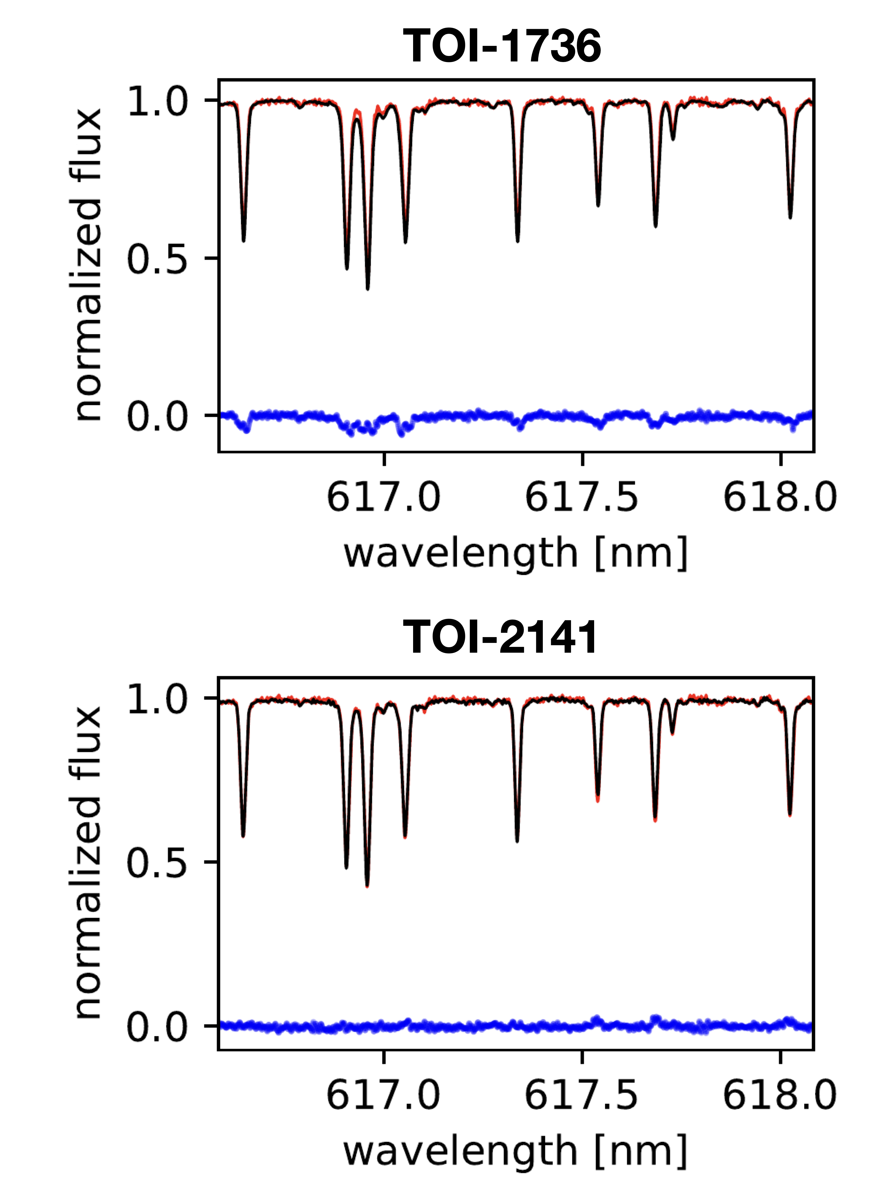
To estimate the errors introduced by instrumental instabilities, we calculated a stacked spectrum from the mean of a randomly selected subsample containing half of the available spectra, where we performed the differential analysis. We repeat this procedure 30 times. As a result, our EWs measurements are stable at % level, which translates into 7 K, 0.02 dex and 0.01 dex in , and [Fe/H]. These are considered the minimum uncertainties achievable by our automatic differential technique applied to the SOPHIE data. Thus, we added these errors quadratically to the internal errors of our measurements.
To estimate possible offsets in our spectroscopic parameters and validate the error analysis, we applied the same spectroscopic analysis to observations of the Moon and to a small subset of 5 previously characterized solar analogs bracketing our sample stars’ parameters, namely: HIP 7585, HIP 28066, HIP 29432, HIP 77052, and HIP 79672. The comparison stars’ literature parameters were obtained from Spina et al. (2018) (hereafter S18) which was based on the same line list of this work and used a similar spectroscopic technique. The differences between our analysis and those from S18 are the higher S/N (500-1000) and the higher spectral resolution (R=120000) from their HARPS data. In addition, the authors performed manual EW line measurements, in contrast to our automatic procedure. Therefore, in terms of internal achievable error levels, we can assume their measurements as noise-free in comparison to ours. In Table 9 we report the comparison between SOPHIE and S18 atmospheric parameters. The typical precision achieved by S18 are K, dex, and dex. Our results agree with their estimates with an average offset of K, dex, and dex. Yana Galarza et al. (2019) also validated their measurements with those in the literature using the same technique as in our work and using instrumentation with similar spectral resolution and higher signal-to-noise ratio (R=60000, S/N400) compared to our SOPHIE data. The authors reported an rms of 12 K, 0.03 dex and 0.02 dex for , , and [Fe/H], respectively. In a similar fashion, S18 found an rms of K, dex, and dex. These results are in line with our differential atmospheric parameters, highlighting the robustness of our methodology applied to similar Sun-like stars.
| Star | |||||||
|---|---|---|---|---|---|---|---|
| ID | (interf)aaaaEffective temperatures for the available sources obtained through interferometry. | SOPHIEbbbbSpectroscopic parameters from our differential analysis. | S18ccccSpectroscopic parameters from Spina et al. (2018) (S18). | SOPHIEbbbbSpectroscopic parameters from our differential analysis. | S18ccccSpectroscopic parameters from Spina et al. (2018) (S18). | SOPHIEbbbbSpectroscopic parameters from our differential analysis. | S18ccccSpectroscopic parameters from Spina et al. (2018) (S18). |
| HIP 7585 | |||||||
| HIP 28066 | |||||||
| HIP 29432 | |||||||
| HIP 77052 | |||||||
| HIP 79672 | |||||||
Finally, to evaluate the accuracy of our methodology, we derived the solar atmospheric parameters from another moonlight spectrum obtained with the same instrumental setup reported in this work. Solar observations were analyzed following the same steps used to determine the parameters of solar analogs. We show in Table 10 the accuracy test using moonlight observations and final differential atmospheric parameters for TOI-1736 and TOI-2141. The agreement with our solar reference values used in q2 confirms the differential analysis as accurate and precise, assuming there is negligible unaccounted-for residual systematics from the reduction process, for example.
| Parameter | TOI-1736 | TOI-2141 | Sun (Moon) |
|---|---|---|---|
Appendix C Activity indices
This appendix details our S-index and Hα measurements. It also shows the time series analysis and RV correlation of the activity indices obtained from the SOPHIE spectra of TOI-1736 and TOI-2141.
C.1 S-index
We computed the SOPHIE’s instrumental S-index as follows:
| (2) |
where and are the integrated fluxes of two triangular band-passes in a 0.109 nm wide window centered on the H (396.85 nm) and K (393.37 nm) Ca II emission lines, and and are two continuum regions 2 nm wide centered at 390.107 nm and 400.107 nm, as illustrated in Figures 24 and 25. For the computation of , we performed flux integration using spectral values generated via Monte Carlo (MC) sampling from a normal distribution, taking into account the central value and errors associated with each spectral element. Figures 24 and 25 depict the posterior distributions for the MC samples.
To calibrate SOPHIE’s instrumental S-index to the Mt. Wilson Observatory (MWO) system (, Wilson 1968; Egeland et al. 2017), we downloaded archival spectra of ten selected stars that are known to have measurements in the range of 0.15 to 0.36. We only used observations in HR mode and with a peak S/N100 in the first order, and we computed the S-index for each calibrator in the same way as described above. We least-square fit a linear relationship between and the values from Duncan et al. (1991), and then we sampled the posterior distribution of the linear coefficients using a Bayesian MCMC framework with the package emcee (Foreman-Mackey et al. 2013) as shown in figures 22 and 23. The best solution is expressed as follows:
| (3) |
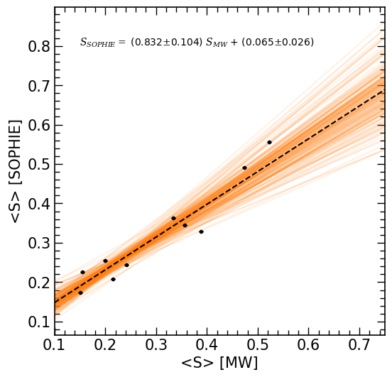
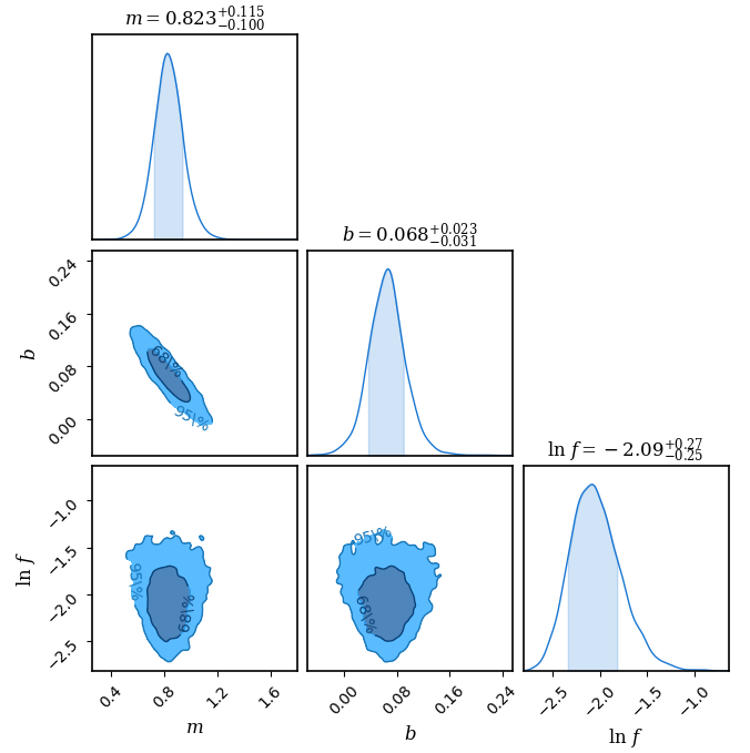
This calibration is consistent with the previous calibration obtained by Boisse et al. (2010). The values from Duncan et al. (1991) and our measurements of for our sample of calibrators are listed in Table 11. Solving Equation 3 to get the for our two stars, we obtained for TOI-1736 and for TOI-2141, where the values were measured in the template spectrum of each target. We have also measured the for each individual exposure, providing the S-index time series for both stars as presented in Tables LABEL:tab:sophiervstoi1736 and LABEL:tab:sophiervstoi2141.
| ID | (SOPHIE) | (MW) | ||
|---|---|---|---|---|
| HD097334 | 0.3449 | 0.0022 | 0.356 | 0.012 |
| HD101501 | 0.3635 | 0.0023 | 0.334 | 0.002 |
| HD114378 | 0.2438 | 0.0015 | 0.241 | 0.005 |
| HD114710 | 0.2549 | 0.0016 | 0.200 | 0.010 |
| HD115404 | 0.5558 | 0.0040 | 0.523 | 0.044 |
| HD131156 | 0.4912 | 0.0035 | 0.473 | 0.010 |
| HD141004 | 0.2254 | 0.0014 | 0.155 | 0.021 |
| HD152391 | 0.3288 | 0.0020 | 0.389 | 0.036 |
| HD182101 | 0.2080 | 0.0012 | 0.215 | 0.013 |
| HD187013 | 0.1745 | 0.0010 | 0.151 | 0.005 |
C.2 H
The H index is calculated from the flux at the center of the H line as described by Boisse et al. (2009), that is,
| (4) |
where is the integrated flux measured within a 0.068 nm window centered at 656.2808 nm, and are the integrated fluxes measured near the edge of the H wings centered at 655.087 nm and 658.031 nm with rectangular band-passes in 1.075 nm and 0.875 nm wide windows, as illustrated in Figures 24 and 25. In a similar way to the S-index calculation, the integration of spectral regions for H calculation employs a Monte Carlo sampling approach. The H indices measured in the template spectra are for TOI-1736 and for TOI-2141, and the individual measurements per exposure are listed in Tables LABEL:tab:sophiervstoi1736 and LABEL:tab:sophiervstoi2141.
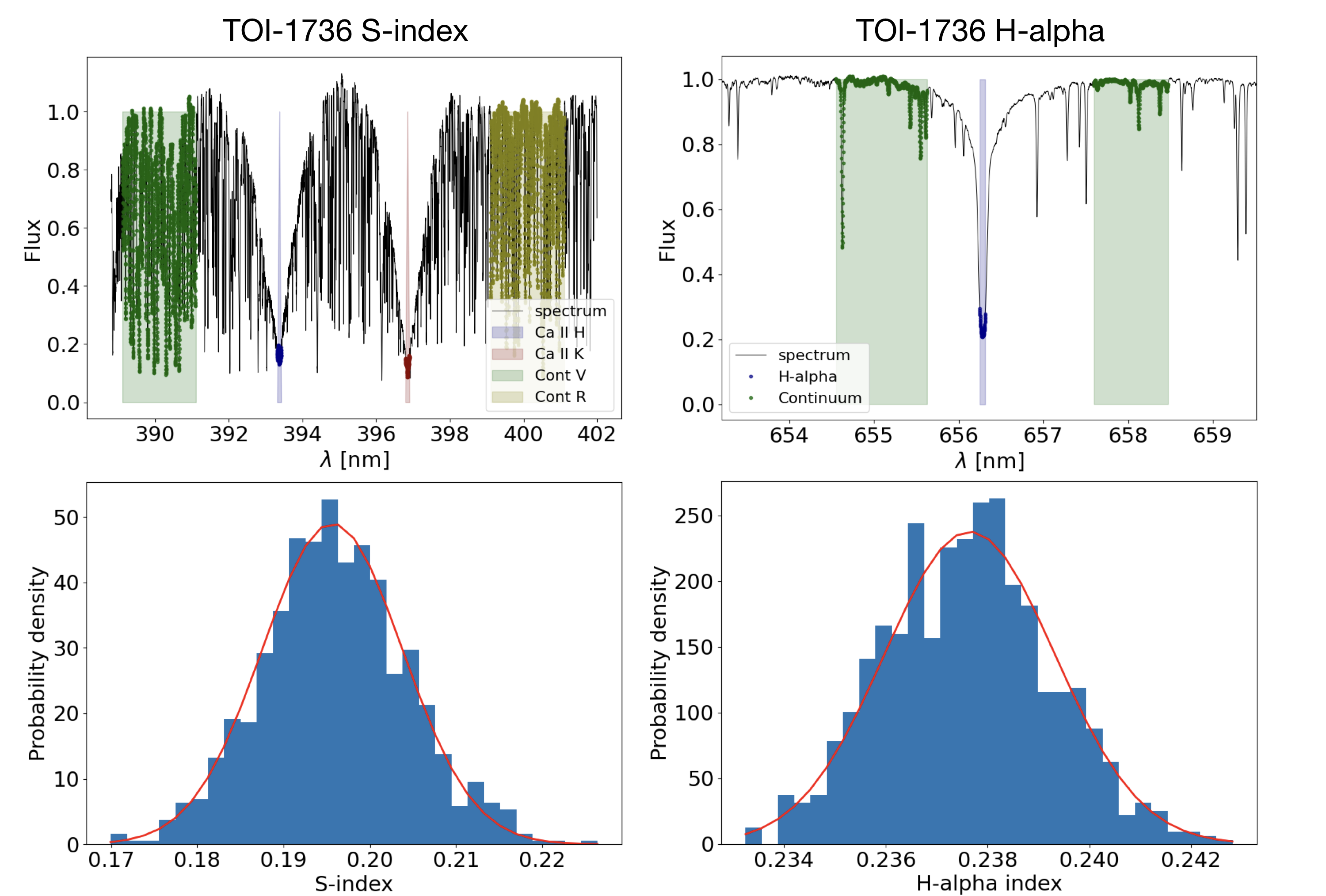
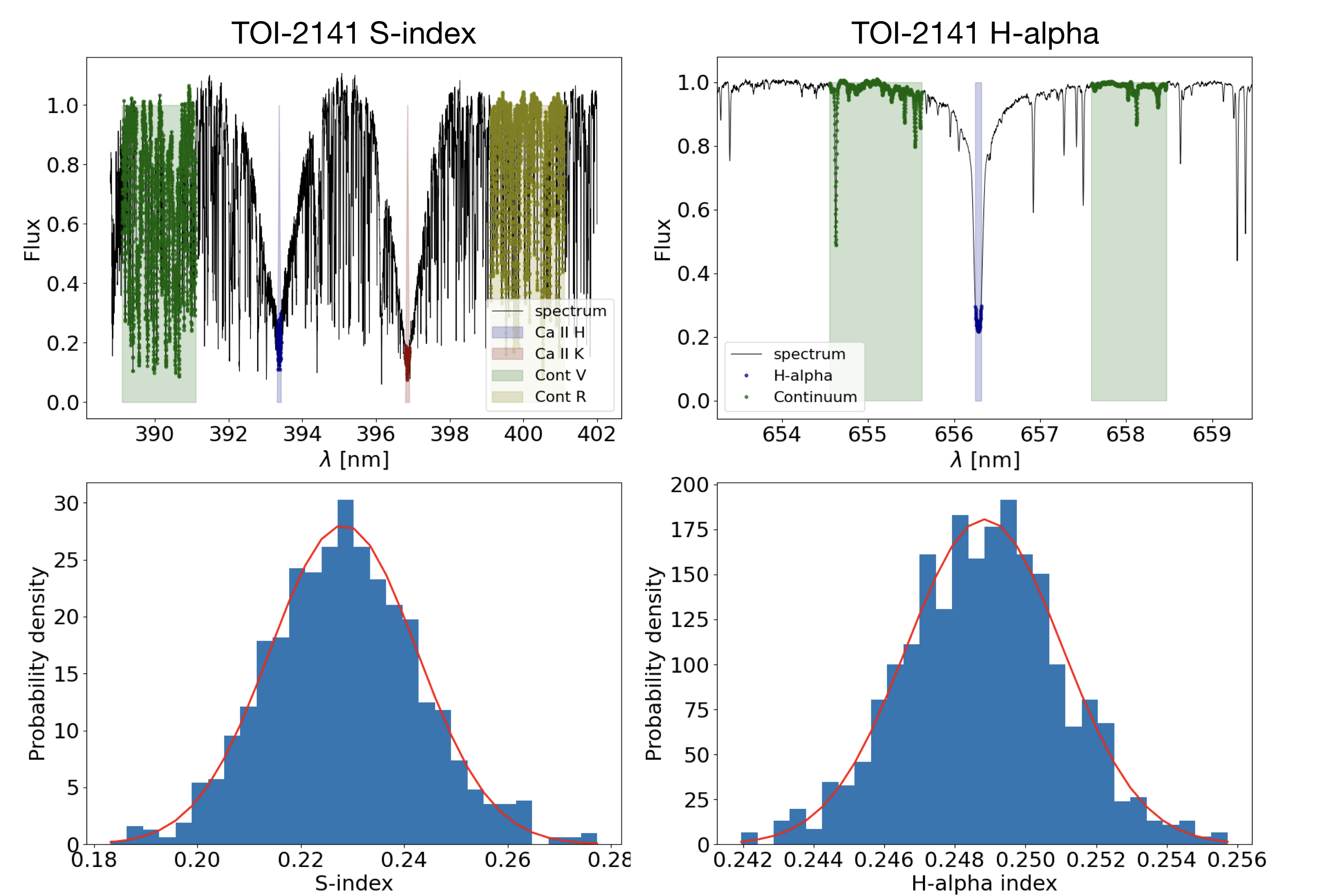
C.3 Time series of activity indices
As star rotation can modulate RVs and activity indices, we can analyze these quantities together and compare their time series and respective GLS periodograms in an attempt to find possible signals that can be used to infer the star rotation period. Figures 26 and 27 show the time series data and the GLS periodograms for both stars, where we cannot identify any significant periodicity. The residual RVs of TOI-1736 show a peak with a false alarm probability greater than 0.001 at 25 d, which may be related to star rotation, but this peak does not appear in any other indices. As such, we could not find any strong evidence for the star’s rotation period from these data.
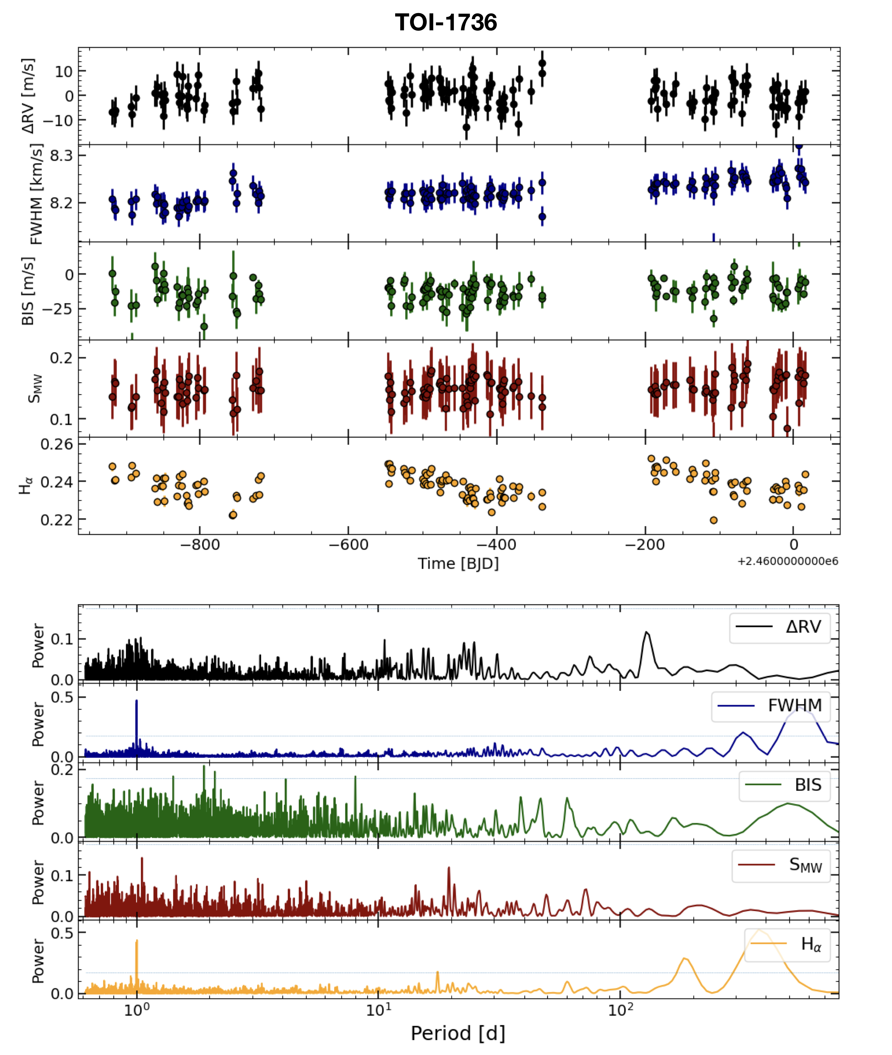
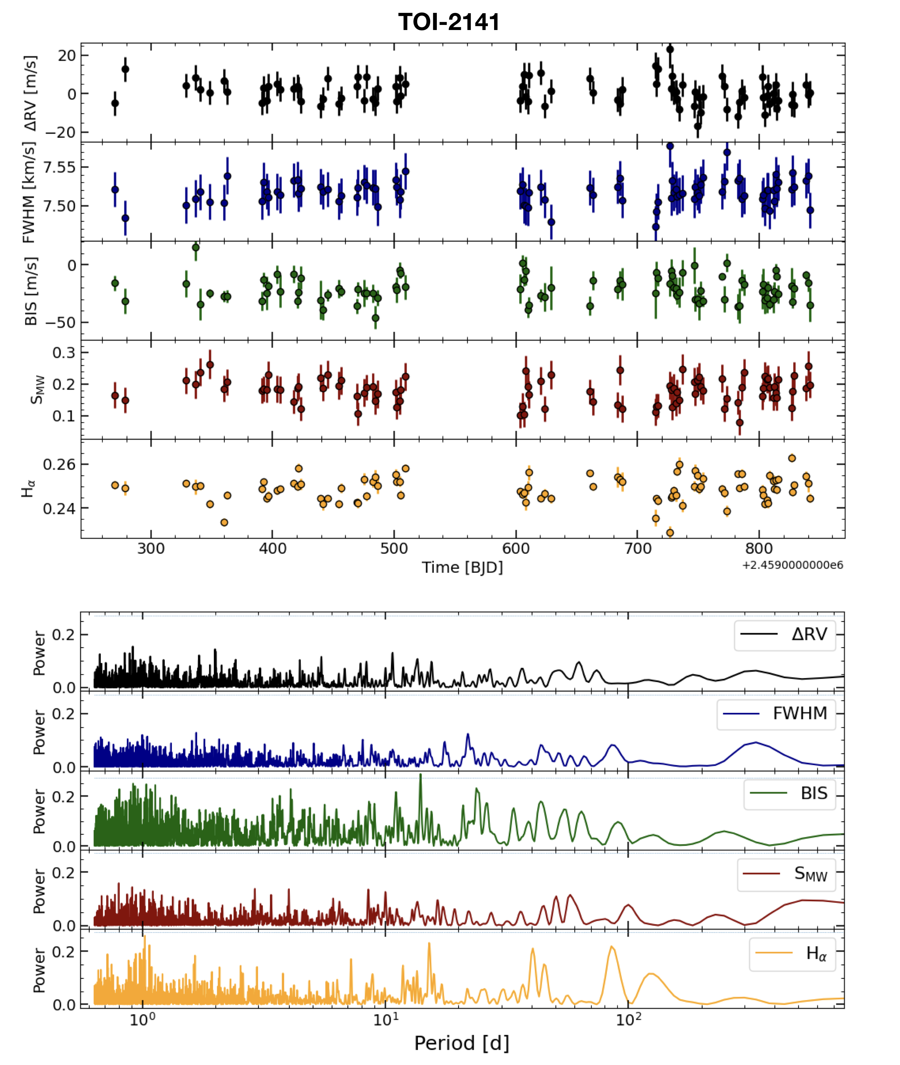
C.4 Correlations between activity indices and RVs
Stellar activity can change the shape of line profiles and lead to deterioration in the detection of planetary signals, or even to spurious detections. One way to inspect the impact of certain types of activity on RV measurements is to look at the correlation between the RVs subtracted from the best-fit RV orbit model and the activity indices. Here, we present these correlations for the CCF FWHM, bisector span, Hα, and S-index, as illustrated in Figures 28 and 29. As pointed out in the main text, there is no strong correlation between these quantities, which indicates that our RVs are not strongly affected by stellar activity.
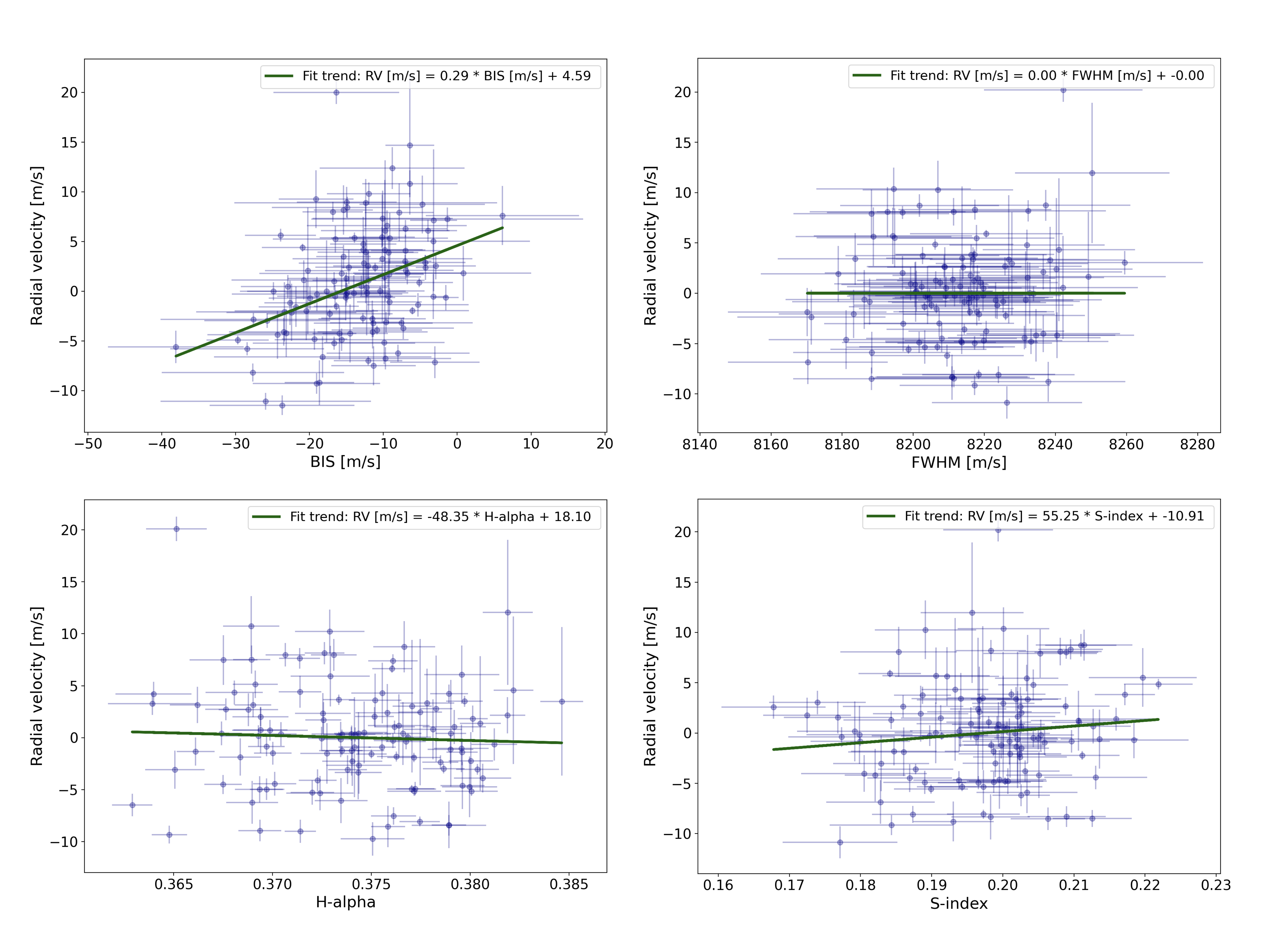
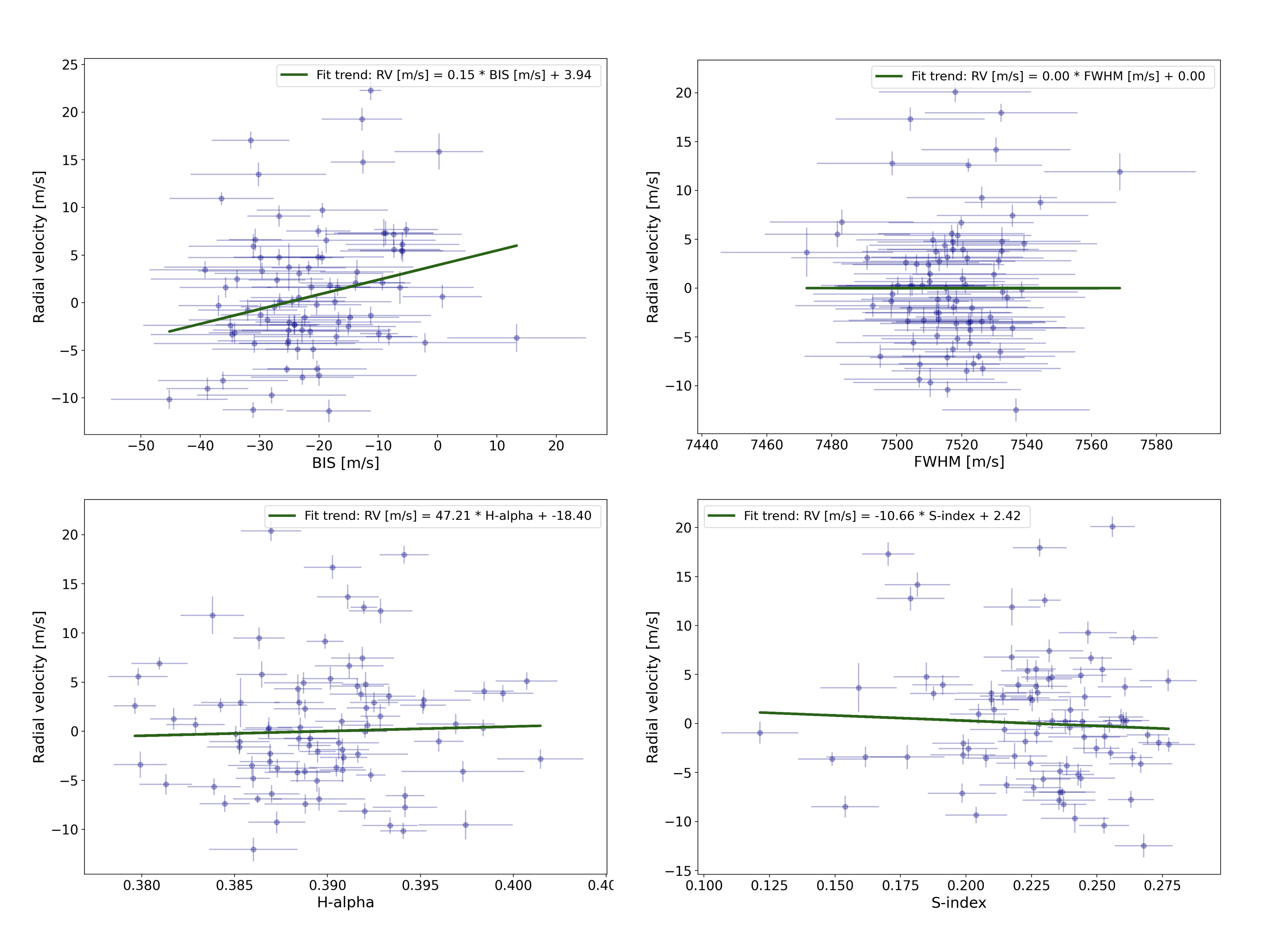
Appendix D Priors and posterior distributions of model parameters
This appendix presents in Table 12 the prior distributions adopted for each model parameter that we considered in our analysis. Figures 30 and 31 illustrate the MCMC samples and the final posterior distributions of free parameters used in our analysis.
| Parameter | TOI-1736 b | TOI-1736 c | TOI-2141 b |
|---|---|---|---|
| time of conjunction, (BJD) | |||
| orbital period, (d) | |||
| eccentricity, | FIXED (0) | FIXED (0) | |
| argument of periastron, (deg) | FIXED (90) | FIXED (90) | |
| normalized semimajor axis, | |||
| orbital inclination, (deg) | |||
| planet-to-star radius ratio, | |||
| velocity semi-amplitude, (m s-1) | |||
| linear limb dark. coef., | |||
| quadratic limb dark. coef., | |||
| systemic radial velocity, (km s-1) | |||
| slope of linear trend, (m s) | FIXED (0) | ||
| GP phot. mean, (ppm) | |||
| GP phot. white noise, (ppm) | |||
| GP phot. amplitude, (ppm) | |||
| GP phot. decay time, (d) | FIXED (10) | FIXED (10) | |
| GP phot. smoothing factor, | FIXED (0.1) | FIXED (0.1) | |
| GP phot. period, (d) | |||
| Parameter | TOI-1736 | TOI-2141 |
|---|---|---|
| GP phot. mean, (ppm) | ||
| GP phot. white noise, (ppm) | ||
| GP phot. amplitude, (ppm) | ||
| GP phot. decay time, (d) | 10 | 10 |
| GP phot. smoothing factor, | 0.1 | 0.1 |
| GP phot. period, (d) |

