Titolo
Abstract
We answer the question: If a vacuum sector Hamiltonian is regularized by an energy cutoff, how is the one-kink sector Hamiltonian regularized? We find that it is not regularized by an energy cutoff, indeed normal modes of all energies are present in the kink Hamiltonian, but rather the decomposition of the field into normal mode operators yields coefficients which lie on a constrained surface that forces them to become small for energies above the cutoff. This explains the old observation that an energy cutoff of the kink Hamiltonian leads to an incorrect one-loop kink mass. To arrive at our conclusion, we impose that the regularized kink sector Hamiltonian is unitarily equivalent to the regularized vacuum sector Hamiltonian. This condition implies that the two regularized Hamiltonians have the same spectrum and so guarantees that the kink Hamiltonian yields the correct kink mass.
Cut-Off Kinks
Jarah Evslin***[email protected]1,2, Andrew B. Royston†††[email protected]3 and Baiyang Zhang‡‡‡[email protected]4
1) Institute of Modern Physics, NanChangLu 509, Lanzhou 730000, China
2) University of the Chinese Academy of Sciences, YuQuanLu 19A, Beijing 100049, China
3) Department of Physics, Penn State Fayette, The Eberly Campus, 2201 University Drive, Lemont Furnace, PA 15456, USA
4) Institute of Contemporary Mathematics, School of Mathematics and Statistics, Henan University, Kaifeng, Henan 475004, P. R. China
1 Introduction
The conventional approach [1, 2, 3, 4] to the computation of the mass of a quantum soliton is as follows. One begins with a Hamiltonian which defines a theory and introduces a one-soliton sector Hamiltonian that describes the same physics in terms of the field expanded about the classical soliton solution. Both Hamiltonians are then regularized.111In the canonical transformation approach of [5], one applies the transformation to a perturbative sector Hamiltonian that includes counterterms. The Hamiltonian is not regularized, however, because it is not expressed in terms of a regularized set of degrees of freedom – Fourier modes up to a cut-off momentum, for example. One defines the soliton mass to be the difference in the eigenvalues between a soliton ground state computed using the one-soliton sector Hamiltonian and the vacuum computed using the original vacuum Hamiltonian. This mass depends on the regulators of both Hamiltonians. Then the regulators must both be taken to infinity. Unfortunately the mass found depends on the choice of how these two regulators are matched as they are taken to infinity [6].
Many prescriptions for this matching have been given in the literature, some leading to the right or the wrong answer. In particular, a cut-off regularization of both Hamiltonians with a matching of the cut-off energies leads to the wrong answer [6].
Several proposals for resolving this problem have appeared in the literature. The dependence on the regulator matching condition arises because of the sharp dependence of the energy on the regulator, which in turn is due to the quadratic ultraviolet divergence in the one-loop energies. In Ref. [7] the authors noted that this problem could be removed by calculating not the energy itself, but rather its derivative with respect to an energy scale, as its divergence will be suppressed by one power. In models simple enough for the constant of integration to be fixed using dimensional analysis, this allows the kink mass to become regulator independent and so one arrives at the right answer, even with the wrong regulator matching condition. While this approach is sufficient for the calculation of the mass in many models of interest, it is not applicable to models with multiple scales and it cannot be used to calculate quantities with a steeper dependence on the energy scale.
These shortcomings motivated Ref. [8] to try to design a prescription for an energy cutoff that would reproduce the known one-loop kink mass. This led them to an appealing physical principle, that normal modes sufficiently above the regulator scale should not be affected by the soliton. Unfortunately this principle alone is not enough to fix the mass, as one must also choose how the density of states scales at high energies and the mass obtained depends on this choice.
The origin of the above difficulties is clear. In standard approaches, one transforms an unregularized defining Hamiltonian to the soliton sector and then regularizes, whereas one should apply the transformation directly to the regularized defining Hamiltonian. For example, the original and accepted result for the one-loop correction to the soliton mass in theory [1] was obtained using mode number regularization. Periodic boundary conditions for a box of size are applied to the relevant fluctuation operator in each sector, and the same number of modes is kept in determining the contribution to the energy. This procedure is motivated by the lattice, but the full Hamiltonian was not defined on a lattice in [1]. If it had been, and the map between sectors given within this defining theory, then there would be no ambiguity in determining how the perturbative and soliton sector regulators are related. While -theory has certainly been studied on a finite spatial lattice starting with [9], where the authors were interested in the phase structure of the vacuum, a lattice version of the transformation from perturbative to soliton sectors has not been developed.
A satisfactory resolution to the above issue, then, is to provide a finite-dimensional lattice version of the soliton-sector canonical transformation given in [5, 10]. This is the approach we will follow in a forthcoming paper. It is conceptually straightforward but technically nontrivial, and one might ask if the same idea –transforming the regularized Hamiltonian to the soliton sector– can be accomplished with a defining Hamiltonian regularized by an energy (or momentum) cutoff. This paper answers in the affirmative.
Our work here follows in the footsteps of [8] in that we want to a obtain a consistent energy cut-off regularization and renormalization for kinks in 1+1 dimensions. Like them, we recognize that the kink profile and the normal modes will depend on the regulator and in a consistent treatment these dependencies should be considered, at least to be sure that they do not affect the answer to any given question. However unlike them, we make no conjectures. We derive our answer, as follows.
Consider a real scalar field . Let be the classical kink solution. The quantum theory will be treated in the Schrodinger picture, and so fields will be considered at a fixed , and the argument will be dropped from the notation. Now it is conventional to expand about the classical solution as
| (1.1) |
In this case one could rewrite the Hamiltonian in terms of the quantum field [11].
We will choose a different approach. It is convenient to expand the field not about but about a zero value of the field, so that higher moments of the field correspond to interactions. This could be achieved using a passive transformation of the field . Instead, following [1], we will employ an active transformation of the Hamiltonian and momentum functionals which act on the field. In particular we will transform the Hamiltonian as
| (1.2) |
This definition of is sufficient for classical field theory, but in quantum field theory is regularized and we would like to define a regularized .
The observation that underlies this paper is that (1.2) is a unitary equivalence. More specifically, we construct a unitary operator which maps the vacuum sector to the kink sector [12, 13]. We define the regularized kink sector Hamiltonian by conjugating the defining, regularized vacuum-sector Hamiltonian with this operator
| (1.3) |
In this sense, the momentum cutoff in the kink sector is inherited from the vacuum sector. Since the two Hamiltonians are similar, they will have the same eigenvalues and their eigenvectors, which differ by the operator , represent the same states. The kink mass is the difference between the eigenvalues of the eigenstates corresponding to the vacuum and the kink ground state. These two eigenstates may be identified in either Hamiltonian, as they have the same eigenvalues and states, however in perturbation theory we may only find the vacuum as an eigenvector of the vacuum Hamiltonian and the kink ground state as an eigenvector of the kink Hamiltonian. In other words, once we have used perturbation theory to find the kink ground state as an eigenstate of then the corresponding eigenstate of the defining Hamiltonian is
| (1.4) |
Note that this approach is not sensitive to the exact choice of . Any which allows one to find the desired eigenvectors of is sufficient, since they all have the same eigenvalues and the eigenvectors are easily mapped between the various eigenspaces using .
The regulator can then be taken to infinity unambiguously, using the renormalization conditions, to arrive at the renormalized kink mass. This limit is unambiguous as there is only one regulator which needs to be taken to infinity, not two. The similarity transformation (1.3) guarantees the correct regulator for the kink Hamiltonian. Previous approaches to an energy cutoff in these models failed222In Ref. [6] it was shown that they yield the wrong one-loop kink mass. because they regularized the kink sector Hamiltonian by imposing an energy cutoff in the spectrum of normal modes, but we will see that includes all normal modes.
In this work we only include an ultraviolet (UV) regulator since the computations considered will not require infrared (IR) regularization. In forthcoming work we will present a soliton-sector transformation for a finite-dimensional lattice regularization that uses both.
Infrared (IR) regularization via compactification or the inclusion of antisolitons is common in the literature. However, such IR regularization is necessarily different for the vacuum and soliton sectors, which makes it difficult to treat nonperturbative effects which mix distinct sectors. Mixing may seem unimportant at weak coupling, but at strong coupling it is responsible for the symmetry restoring phase transition in the theory. Also the dual Thirring description for the Sine-Gordon model includes a mixing of two-fermion and zero-fermion states.
We begin in Sec. 2 by defining the regularized theory and the vacuum sector. Next in Sec. 3 we define the similarity transform which takes the defining Hamiltonian to the kink sector Hamiltonian. Finally in Sec. 4 we find the regularized kink sector Hamiltonian and calculate its one-loop ground state and mass. When the regulator is taken to infinity, we reproduce the known mass formula. Our notation is summarized in Table 1.
| Operator | Description |
|---|---|
| The real scalar field and its conjugate momentum | |
| Creation and annihilation operators in plane wave basis | |
| Creation and annihilation operators in normal mode basis | |
| Creation/annihilation operators of odd shape modes | |
| Zero mode of and in normal mode basis | |
| Normal ordering with respect to operators respectively | |
| Hamiltonian | Description |
| The original Hamiltonian | |
| with shifted by regularized kink solution | |
| The term in | |
| Symbol | Description |
| Momentum cutoff | |
| The unregularized classical kink solution | |
| First correction to the unregularized classical kink solution | |
| Regularized classical kink solution | |
| Operator that translates by the regularized classical kink solution | |
| The kink linearized translation mode | |
| Normal modes including discrete modes | |
| Momentum | |
| Normal mode label | |
| The frequency corresponding to or | |
| Inverse Fourier transform of | |
| State | Description |
| Kink and vacuum sector ground states |
2 The Vacuum Sector
2.1 Classical Theory
Let us consider a classical theory of a real scalar field and its conjugate in 1+1 dimensions,
| (2.1) |
where we have included counterterms and and a potential which in the case of the double well theory is
| (2.2) |
The potential is always written as a function of because this combination is dimensionless. The notation emphasizes that the quantity in question depends on the regulator . In this note we will focus on the theory, where renormalization conditions can be chosen such that the coupling is not renormalized and the only required counterterms are those proportional to and [6]. However the strategy can be readily generalized to other potentials by adding counterterms for the additional interactions and corresponding renormalization conditions.
We will be interested in cases in which has multiple minima, so that there is a kink solution in the classical theory. To simplify the discussion below, we will shift the field by the location of one of these minima, by defining
| (2.3) |
leading to
| (2.4) |
In the case of the double well one obtains
| (2.5) |
2.2 Quantum Theory
As the action has the dimensions of , the operator has dimensions while has dimensions . Therefore also has dimensions . This means that in the quantum theory, they will appear in the dimensionless combinations and . Thus in the semiclassical expansions below, each power of will be treated as one power of .
We will not directly quantize and . Instead we will decompose
| (2.6) |
and we will quantize and by imposing
| (2.7) |
This note will be entirely in the Schrodinger picture, and so (2.7) defines Schrodinger operators and . They are not local fields; indeed they satisfy
| (2.8) |
The nonlocality of the commutator arises from the fact that the integration in the momentum space is cut off by . Note that locality is restored as the cutoff is removed because
| (2.9) |
Interestingly, (2.8) are the same canonical commutation relations found in Pearson’s thesis [14] (see also [15]) for an infinite lattice regularization with lattice spacing . In this context, are interpolating fields for underlying lattice degrees of freedom that do satisfy canonical commutation relations. Using the interpolating fields to define the regularized Hamiltonian, as we have done here, implies that our theory is equivalent to the infinite lattice theory of Pearson. We do not utilize the lattice language in this paper since it is not advantageous for the computations we perform. We will utilize it, however, in forthcoming work when we construct a finite-dimensional version of the soliton-sector canonical transformation.
Our problem is now well-defined. One can insert (2.6) into (2.4) to obtain the Hamiltonian as a function of the operators and . The vacuum and the kink ground state will be eigenstates of this Hamiltonian, and the difference between their eigenvalues is the kink mass. The Schrodinger picture is sufficient for determining the spectra and so we need never introduce time, and the nonlocality of our operators will not impede our narrow task.
To do this concretely, we will choose the renormalization condition
| (2.10) |
and will expand
| (2.11) |
Let us begin with the case . We are interested in terms in with no powers of . Let us assume for the moment that contains only terms of order at least . We will see shortly that this choice is consistent. Then we are left with
| (2.12) | |||||
For the double well, . Define the linear combinations
| (2.13) |
where the Hermitian conjugate of is . The canonical commutation relations (2.7) imply that these each satisfy a Heisenberg algebra
| (2.14) |
To impose (2.10) at , it suffices to consider which is the free vacuum
| (2.15) |
The definitions (2.13) are easily inverted
| (2.16) |
Substituting this into (2.12) one finds
| (2.17) |
and so the leading order counterterm is
| (2.18) |
where we have integrated by parts. We have now satisfied the renormalization condition (2.10) at order .
To fix we will impose another renormalization condition, that tadpoles vanish. Recall that is a series in beginning at order . For the computation of these leading order terms, the no-tadpole condition is equivalent to imposing that contains no terms of the form at . The relevant terms in the Hamiltonian are
| (2.19) |
where is the th derivative of and we recall that is of order .
Using the terms with a single
| (2.20) |
one obtains
| (2.21) |
In the case of the double well this is
| (2.22) |
2.3 The Relation to Normal Ordering
One may define a normal ordering on the operators and by placing all of the former on the left. We will denote this normal ordering for any operator . It is easily evaluated on the operators appearing in the Hamiltonian at the orders considered above
| (2.23) | |||||
Inserting these into (2.12) and (2.19) one finds
| (2.24) |
We see that order by order, properly chosen renormalization conditions are equivalent to a Hamiltonian that is normal ordered from the beginning. More specifically, the required renormalization condition sets to zero all diagrams with a loop involving a single vertex. In the case of two-dimensional scalar field theories, normal ordering is sufficient to remove all divergences (see for example Ref. [16]). Thus it would be possible to take the limit now. This would reduce the problem to that solved already in Ref. [17, 18] at one loop and [19] at two loops where it was shown that one arrives at the correct kink mass. However, we will not follow this approach as it will not generalize to theories with fermions and theories in higher dimensions, which motivate this line of research.
In the case of the theory, with the renormalization conditions of Subsec. 2.2, the total Hamiltonian density is then
| (2.25) |
Here we have shifted the subleading counterterm to absorb the contribution from Wick contractions appearing in the normal ordering of the interaction
| (2.26) |
In Refs. [20, 21], the calculation of was reviewed and it played an essential role in the elimination of IR divergences in the calculation of the two-loop kink mass. The shifted counterterm and all successive terms are finite at , with the first few given in Eq. (47) of Ref. [22]. In the case of a general potential, normal ordering again leads to such infinite shifts and finite remainders.
3 Defining the Kink Sector
3.1 The Similarity Transformation
Let be a real-valued function. Define the displacement operator
| (3.1) |
and
| (3.2) |
This integral is often divergent. Our prescription for defining in this case is described in Appendix A.
Exponentiating the commutators
| (3.3) |
and
| (3.4) |
one finds
| (3.5) |
Therefore
| (3.6) |
where
| (3.7) |
satisfies if for all with . Note that commutes with as .
Finally we are ready to introduce the similarity transformation at the heart of our construction. The kink sector Hamiltonian is defined by
| (3.8) |
for a suitable choice of , which will be made momentarily. In the rest of this note we will be concerned with . As it is similar to , it has the same spectrum. In particular if
| (3.9) |
then, using (1.4),
| (3.10) |
and so may be used to compute the energy of any state, and in particular the energy of the kink ground state.
3.2 The Kink-Sector Tadpole
Let us consider to be of order . Then the kink sector Hamiltonian can be expanded order by order in the coupling
| (3.11) |
where each and is of order . At leading order one finds the classical energy corresponding to the field configuration
| (3.12) |
The kink-sector tadpole appears at the next order:
| (3.13) |
We will define by imposing that the expression in brackets vanishes at momenta below the cutoff333Note that, although the higher modes of vanish, those of the term do not vanish. However they do not contribute to the tadpole in Eq. (3.13) as the higher modes of vanish.
| (3.14) |
which will automatically eliminate the kink sector tadpole as satisfies the opposite condition
| (3.15) |
In the case this condition corresponds to the classical equations of motion for a time-independent configuration in the unregularized theory. Thus will be equal to the classical kink solution and will reduce to its classical mass density.
The definition (3.14) can be solved as an expansion in large about the classical solution . To illustrate this procedure, in Appendix A we find the leading correction in the case of the double well and show that it is exponentially small in .
4 The Kink Sector
4.1 The Setup
In this section we will restrict our attention to the double well theory. As noted above, an analogous treatment of models with other interactions generically requires additional counterterms multiplying various powers of . Inserting (2.25) into (3.8) one finds that the -independent terms are
| (4.1) |
These are the only terms that contribute at one loop, as they are suppressed by a factor of with respect to the leading terms in and we have chosen so that vanishes. The term is -independent and becomes as . However, we argued in Appendix A that the corrections are exponentially small in . Since perturbative computations only produce power-law divergences in , such exponentially small corrections do not contribute to any perturbative quantities. Therefore in the following we will replace with .
For completeness we note
| (4.2) | |||||
In the rest of this note we will use (4.1) to study the one-loop kink spectrum. This equation describes a theory which is free, as the Hamiltonian is quadratic in the field. However the operators and do not diagonalize the Hamiltonian as a result of the -dependent mass term. Our strategy will thus be to diagonalize using a Bogoliubov transformation from the basis of operators that create plane waves to a basis of operators that create normal modes of the regularized kink.
First let us find these normal modes. Inserting the Ansatz444This constant frequency Ansatz is inconsistent with the restriction that the higher Fourier modes of vanish. However, when we construct the quantum field below, we will consider only those linear combinations which satisfy the restriction. The key observation will be that these combinations do not have constant frequency, and so our regularized kink Hamiltonian is not obtained by cutting off frequencies above any sharp threshold.
| (4.3) |
into the classical equations of motion for (3.8) one finds
| (4.4) |
The index will include a continuous spectrum with energy
| (4.5) |
as well as discrete modes. In the case of the modes there are two discrete solutions, the zero mode corresponding to the translation symmetry with and also an odd shape with .
As is real we may choose
| (4.6) |
and so is real, is imaginary and in the case of continuum modes
| (4.7) |
We normalize the solutions such that
| (4.8) |
and in the case of continuum modes
| (4.9) |
These satisfy the completeness relation
| (4.10) |
From here on we will adopt the shorthand that implicitly includes a sum over the discrete modes and . We also introduce the inverse Fourier transform
| (4.11) |
The completeness relation (4.10) implies that the functions are a basis of all functions so we may decompose
| (4.12) |
Recall that the integral implicitly sums over bound states, and so for example we have also introduced and . Note that the integrals are never cut off.
As the integral is bounded, the field satisfies the constraint
| (4.13) |
The integral is not bounded, indeed including the discrete sums it runs over a complete basis. Therefore (4.13) implies a constraint on the coefficients
| (4.14) |
Here we see the difference between our approach and the traditional mode matching [1] or energy cut-off [6] regularization schemes. In the traditional approach, one limits the integration to include either the same number of modes as in the integration or else an integral out to the same energy. Here instead we integrate over all but with a constraint on the coefficients which leads these coefficients to be small555The are operators. They are small at large in the sense that they are superpositions of with small coefficients. at but nonzero. We claim that this is the correct way to regularize the kink Hamiltonian with a UV energy cutoff because in this approach the regularized kink Hamiltonian is related by a similarity transformation to the vacuum Hamiltonian, which defines the theory. In particular they have the same spectrum, and thus the kink mass, which is the difference between two eigenvalues, can be calculated using one eigenvalue from each Hamiltonian.
The decompositions lead to the Bogoliubov transformations
| (4.15) |
Integrating (4.12) over with weight666If is a discrete mode, where is the parity of the discrete mode . one finds the inverse transformations
| (4.16) |
4.2 Finding the One-Loop Hamiltonian
consists of three terms
| (4.17) |
First consider the potential term
The derivative term cancels
after integrating by parts twice, leaving
where
Here in the case of a discrete mode with parity , . The contraction term is
The last term in is
where
| (4.24) |
and
| (4.25) | |||||
In all, we see that is the sum of a scalar plus an operator
| (4.26) |
This looks like an infinite sum of quantum harmonic oscillators, however and are not quite canonical variables in the regulated theory as
Nonetheless let us try to solve it as if it were a sum of harmonic oscillators, by defining
| (4.28) |
so that
| (4.29) |
Then we can rewrite the operator part of as
| (4.30) |
The operators and operators automatically solve analogous constraints to (4.14)
| (4.31) |
Summarizing, we may write as the sum of a scalar plus a term which is of the quantum harmonic oscillator form
| (4.32) |
We have argued that at one loop this Hamiltonian completely characterizes the kink sector. In Appendix B we argue that the naive IR divergence in the -number term at vanishes.
If we now set the regulator to infinity, then substituting (2.9) into (4.2) one finds the standard canonical commutation relations
| (4.33) |
We can then easily read off the exact spectrum of the regularized Hamiltonian at one loop. The leading order kink ground state is the state annihilated by all and it has mass given by the first term in (4.32), which, when indeed agrees with the formula in Refs. [11, 17, 18].
Using
| (4.34) |
one finds when , that the excited states can be obtained by acting with , each of which increases the energy by
| (4.35) |
Our compact notation, in which integrals over included sums over discrete states, hid the role of the zero mode. In the case of the zero mode, and so the definition of is singular. However in that case the oscillator (4.26) has no term and so its contribution to is simply the nonrelativistic center of mass kinetic energy . Thus the spectrum therefore also includes various center of mass momenta for the kink. This, together wth the shape and the continuum quantum harmonic oscillator spectrum, yield the known one-loop spectrum of Ref. [1].
4.3 One-Loop Kink Ground State of the Regularized Hamiltonian
The nondiagonal nature of (4.34) means that the normal mode basis does not diagonalize when is finite. Nevertheless, we will show that the ground state is still annihilated by all and hence, even at finite , the one-loop kink mass is given by the first term in (4.32).
Let us go back a few steps to (4.2) and (4.24)
| (4.36) |
Define the eigenstates of the operators as
| (4.37) |
where is a real-valued function on the interval . Let us write the arbitrary state in the Schrodinger representation
| (4.38) |
where the integral is over all functions and is the Schrodinger wave functional. As the eigenstates are a complete basis, the state is arbitrary. It follows that
| (4.39) |
Inserting the Ansatz
| (4.40) |
into (4.36) one finds an expression of the form
| (4.41) |
where
| (4.42) |
Our strategy will be to find the such that and use it to find . A sufficient condition for to vanish is
| (4.43) |
for all and . Multiplying by and integrating over , using completeness of , one finds
| (4.44) |
We claim that this , inserted into the Ansatz (4.40), is the kink ground state, or more precisely . To see this, note that it is annihilated by all :
| (4.45) | |||||
| (4.46) | |||||
| (4.47) |
where the last step follows from (4.43). Hence is annihilated by the last term of (4.32) and since this term is a positive operator must be the lowest energy state. As a check, note that the corresponding energy is
| (4.48) | |||||
which matches the from Eq. (4.30).
Therefore, even in the regularized theory, is the energy contribution from , or more precisely the eigenvalue of the operator acting on the kink ground state. Including the scalar terms in , one finds that the total ground state energy of the regularized kink is
| (4.49) |
This is the ground state energy for the unregularized kink found in Ref. [11] using mode matching, but now with the integral cut off. Therefore the limit agrees with the known result.
5 Remarks
In this paper we have described a quantum model which is regularized by a cutoff from the beginning. It exhibits a quantum kink and we found, at one-loop, its ground state and mass. The results were almost trivial generalizations of the corresponding results in the unregularized theory, in which one merely restricts the domain of integration of the momentum to the interval . This is in part because at one-loop, the theory is free, although it is diagonal in the normal mode basis and not the momentum basis. However this was also suggested by the fact that two-dimensional scalar models can be rendered finite by normal ordering without ever regularizing, and so all quantities may be computed without recourse to regularization [2, 17]. Thus one may already suspect that no sign of regularization may remain when the regulator is taken to infinity, as it could have been avoided from the beginning.
In more interesting models, with fermions or more dimensions, normal ordering is not sufficient to remove all divergences. Thus it is possible that the limit in which the regulator is taken to infinity will leave some nonzero residue, indeed in the case of supersymmetric kinks one may expect to arrive at the contribution from the one-loop anomaly [24].
In the supersymmetric case one may hope that sufficient supersymmetry will allow a nonperturbative approach. However we saw here that the kink solution itself has corrections of order . In perturbation theory, we expect this to be always multiplied by finite powers of and so such contributions will vanish in the limit, but in the nonperturbative regime, which is the relevant regime for applications to paradigms [25, 26, 27] of QCD confinement, it is possible that these corrections will be physically relevant if not dominant.
Appendix A Finding the Shift: The Double Well
In this appendix we evaluate the leading correction to in the case of the double well. We show that it is exponentially small in but nonzero. Here we consider the double well without shifting by as in Eq. (2.3). Recall that, in momentum space, this corresponds a shift of the transformed field by and in particular it only affects the momentum space field at .
In this model the definition (3.14) is
| (A.1) |
The basic approach is to insert the finite- Fourier transform
| (A.2) |
into (A.1). Our Ansatz for is the series expansion
| (A.3) |
where is just the Fourier transform of the classical solution and is bounded, for all , by a polynomial in times . We will then solve for the perturbatively, and along the way will see that our Ansatz is consistent. This will imply the main result of this appendix, that can be expanded in a power series with the leading dependence suppressed by order .
There are, however, two technical points that require explanation before proceeding. First, we must define the symbol in (A.2). Ordinary integration, for a classical kink solution, would be ill-defined at . We are free to define the Fourier transform as we like, so long as we are able to use it to demonstrate the main result written above. Therefore, we choose to be a principal value integral, defined by
| (A.4) |
This type of integral can be used to obtain the standard kink profile from its Fourier transform :
| (A.5) |
The integral on the right would be undefined without the principle value prescription. More generally, as a distribution the Fourier transform acts on any test function via integration against with the principle value prescription. Indeed, the proper setting for the kink profile and its Fourier transform is to view both as tempered distributions. The kink profile, , is a nonsingular distribution, meaning that it is defined globally by a smooth function. The Fourier transform is singular, meaning that it can only be represented locally by a smooth function (the csch above); its definition as a distribution contains more information – namely the principal value prescription. Although we do not a priori know the explicit finite- analogs, and , we we expect they have the same large- asymptotics and the same singularity structure at as the leading order configurations , respectively, hence the appearance of the principal value integral in (A.2).
A second technical point is the following. The standard result for smooth functions that the Fourier transform of the pointwise product is the convolution of Fourier transforms,
| (A.6) |
also holds for tempered distributions,777It holds for distributions when the product is defined. In general this involves a condition on the wave front sets of the distributions [28]. In the case of , which is defined globally by integration against a smooth function, the wave front set is trivial. The product of this distribution with any other temprered distribution is defined and the convolution theorem holds. where the factor of is due to our Fourier transform conventions. Here, if are ordinary functions then denotes the pointwise product and denotes the convolution. The convolution of two distributions is defined through the convolution of a distribution with a smooth test function as follows. If is a distribution defined locally by and a smooth function with compact support, then the convolution is a smooth function with value . The convolution of two distributions is then the unique distribution such that . This definition and the corresponding convolution theorem can be extended to
| (A.7) |
where and the distribution on the right is defined through sequential action on a test function.
An instructive example is to show that (A.6) holds for the kink profile and its Fourier transform. Using , one finds that has
| (A.8) |
Below, we will recover this result in the limit of a finite- computation of the convolution, .
We can think of in (A.2) as the ordinary inverse Fourier transform of if we define to vanish outside of . For example, if , initially defined on all of , is set to zero outside , the resulting distribution is still a tempered distribution (now with compact support). Henceforth we will write for distributions with support on . In particular, for any test function we have
| (A.9) |
The convolution theorem continues to hold for such distributions, so that for powers of we have
| (A.10) |
Note this means that the support of the - convolution must be such that
| (A.11) |
This reflects the fact that the pointwise product of ’s on the left of (A.10) contains momentum modes up to .
With these preliminaries out of the way we can proceed with the perturbative solution of (A.1). Inserting (A.2) into (A.1) gives
| (A.12) |
This is an integral equation for the local function on . We expect the distribution to be singular at and defined via the principal value prescription as discussed above. Therefore, we restrict attention in (A.12) to .
Inserting the expansion (A.3) into (A.12), and assuming that solves the equation when (which we will check), we find the following linear equation for the first correction, :
| (A.13) |
where is the first finite- correction from the non-linear term evaluated on the leading-order solution:
| (A.14) |
Hence the main tasks now are to compute the finite- convolutions of with itself appearing in (A.13), (A.14), and to invert the linear operator in (A.13). In the following we describe the approach and present the results but suppress all intermediate steps.888A more detailed presentation of this calculation may appear elsewhere.
The first convolution we need is , given by
| (A.15) | ||||
| (A.16) |
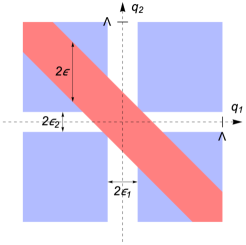
for any smooth test function . We introduce infinitesimal parameters associated with the principal value integrals over respectively, and we can assume since the limit is to be taken first. The basic idea is to change integration variables in the double integral from to , where , and carry out the integral to extract . This, however, is only valid away from , since it involves exchanging the limit with the integral over . If then the factor is not smooth at the pole, and one must take limit first, before evaluating the integral. Therefore we divide the integration into two pieces: one over a region and the other over . We take and send at the very end. See Figure 1.
The integral over gives a result for the right-hand side of (A.15) that is proportional to in the limit , and hence this corresponds to a delta function contribution to . The coefficient can be evaluated and turns out to be -independent, and this term matches the -function term in (A.8). Meanwhile the integral over gives a -dependent contribution. In total we find
| (A.17) |
This agrees with the right-hand side of (A.8) in the limit for fixed , as required by the convolution theorem. It has integrable logarithmic singularities at .
For the double convolution we use
| (A.18) | ||||
| (A.19) |
We apply (A.15) for and change variables in the remaining double integral from to where . Integrating over will then allow us to extract the double convolution . Note there is no principal value prescription required for the distribution as it has no poles. Thus for all it is possible to obtain a local representation of the double convolution by carrying out the integral only. Furthermore, although the support of the double convolution is , we only require it in the range for the solution to (A.12). For any in this range, the integration over covers . Here the outer limits are due to and the inner limits are due to the principal value prescription on the integration. Hence, we have that
| (A.20) |
where the first term arises from the Dirac delta term in (A.15) and we’ve defined
| (A.21) | ||||
| (A.22) |
as giving the contribution from the remaining piece of (A.15). We’ve pulled out an explicit factor of from the definition of so that in (A.14) is precisely the first subleading term (with respect to the exponential behavior) in the large expansion of .
By changing variables , one sees that the second integral in (A.21) is the negative of the first with . Thus is an odd function of . The integral can be evaluated in closed form in terms of logarithms and dilogarithms. We record the full result here since it is important in demonstrating our claim that the perturbative expansion is an expansion in . Setting and for shorthand, we find
| (A.23) | ||||
| (A.24) | ||||
| (A.25) | ||||
| (A.26) | ||||
| (A.27) |
and we have checked this result against numerical integration. Noting that for small , it is easy to see that has a power series expansion in , where every term after the very first one in the curly brackets above begins at :
| (A.28) |
where, for fixed , times a linear function in . Inserting this result back into the double convolution (Appendix A) gives
| (A.29) |
Therefore is indeed the leading order solution to the integral equation, (A.12). Furthermore, we find that the source term in the equation for the first correction, (A.13), is
| (A.30) |
Notice that, while for fixed the source term (A.30) is , it is bounded by a quantity of for all . In particular vanishes at as do all of the .
Now consider the integral operator on the left-hand side of the linearized equation (A.13), which we denote :
| (A.31) |
The double convolution can be written in the same form as (A.18), but with replaced with . The principal value integration from arises from changing variables in the analog of (Appendix A) from to . Thus
| (A.32) | ||||
| (A.33) |
We would like to find an inverse for , whose kernel is a Green function that we denote , for . In order to extract the leading behavior of , however, it is sufficient to find an approximate inverse, whose kernel we denote , such that
| (A.34) |
where we recall that is bounded, odd, and for fixed with .
A standard Neumann series for the inverse, based on the form of (A.32) as a diagonal operator plus “correction,” where the correction is the second term, may not provide a sufficiently good approximation demonstrate this, since the correction is in a neighborhood of the diagonal. A natural ansatz for a better first approximation to is based on its counterpart, which we describe next.
We claim that the approximate Green function can be taken to be the Green function of the standard fluctuation operator, , which we denote by , restricted to . We will discuss the error in this approximation after presenting and its Green function. We have
| (A.35) |
which can be obtained from the Fourier transform of the position space fluctuation operator around the kink:
| (A.36) | ||||
| (A.37) |
for which the eigenmodes are the in (4.4). does not have an inverse due to the zero-mode . It does have an inverse on the orthogonal complement of , whose integral kernel is the Green function satisfying
| (A.38) |
Imposing orthogonality to and exponential fall-off at large , the solution to (A.38) is
| (A.39) |
where and .
Then is the Fourier transform satisfying
| (A.40) |
and we can compute it explicitly:
| (A.41) | ||||
| (A.42) | ||||
| (A.43) | ||||
| (A.44) |
where with the digamma function. Note that .
The regular piece is smooth and bounded on all of . The pole from the csch pre-factor along the diagonal is canceled by a zero from the quantity in curly brackets. For fixed , the large behavior of the quantity in curly brackets is linear and therefore as . Furthermore, along the diagonal, one can show that falls off like for large .
We use these facts to argue that the restriction of to can be taken as the approximate inverse in (A.34):
| (A.45) |
There are two sources of error in this approximation. First there is the error in replacing the inverse of by the inverse of . Then there is the error in approximating the inverse of the latter operator, which we will think of as a restriction of to an upper-left block, with the upper-left block of its inverse.999There is no issue regarding the fact that is only an inverse to on the orthogonal complement to the zero-mode . The reason is that we can restrict interest to acting on functions that are odd on and so are orthogonal to , which is an even function of . We discuss each in turn.
To simplify notation, let be the integral operator we have, and let . Let the difference be with kernel
| (A.46) |
which vanishes along the diagonal and is exponentially small in in a neighborhood of the diagonal. Again, we note the logarithmic singularity at is integrable and has a coefficient that is exponentially small in . Thus we expect the corrections in approximating by from the Neemann series,
| (A.47) | ||||
| (A.48) |
to be exponentially small in .
Now, is the restriction of to functions with support on , while we define as the analogous restriction of , and what we know is that . A finite-dimensional matrix analog of our problem is that we have that
| (A.49) |
are inverses of each other and we would like an expression for . Assuming is invertible, then the finite-dimensional formula from block inversion is
| (A.50) |
We assume the same formula holds in our setting, and we expect to be invertible since it has the form of a diagonal matrix plus a small correction. Then the above remarks on the properties of imply that , with and , is generally exponentially suppressed, except in neighborhoods of the corners where . In these neighborhoods we still have that is bounded by a quantity of . Analogous remarks apply to . Therefore we expect that is suppressed101010In more detail, when are away from the diagonal has double the exponential suppression in the distance from the diagonal as . Along the diagonal, assuming the dominant behavior of is , the contribution of is estimated by an integral of the form , which is . by at least relative to for any . Therefore combining (A.47) and (A.50) we write
| (A.51) |
which gives (A.34).
It follows that the solution to (A.13) for the first correction is
| (A.52) |
Note that for fixed the exponential damping in from the csch pre-factor of balances the exponential growth from the sinh pre-factor of . Since the integrand then grows linearly in at large and the explicit leading dependence of is , one sees that the leading behavior of will be . Since the dependence of the integrand of (A.52) is simple, the leading behavior of the integral can be computed by applying the fundamental theorem of calculus. The result is
| (A.53) | |||
| (A.54) | |||
| (A.55) |
Thus for fixed we have , and for all we have that is bounded by a quantity of .
Since has the same exponentially suppressed form as the source , it follows from the above analysis that the linearized equation for the correction, , will be of the form , where has the same suppression as . Hence will also have the same exponential suppression as , and will generally involve a polynomial in whose degree grows with .
Appendix B IR Divergences
At two or three loops, depending on the theory in general the energy of the kink ground state is IR divergent. More specifically, the Sine-Gordon kink has a divergence at three loops, the kink at two, and if the potential expanded around a minimum corresponding to each end of the kink begins its polynomial expansion at , the first IR divergence will occur at loops. These IR divergences do not affect the kink mass as they also appear, at one less loop, in the vacuum energy and the kink mass is the difference between the two energies.
Here at one loop we found the energy
| (B.1) |
In the cases of the Sine-Gordon and modes, contains a term. One of these functions may be eliminated by the integration over , but the other potentially leaves a divergence already at one loop. In coordinate space, it is easily seen that the origin of this divergence is a constant energy density, and so it is an IR divergence.
Such IR divergences have been noted since the first papers [1] on kink mass calculations, and are usually regularized by compactifying the space using periodic boundary conditions. This is quite a high price to pay111111While the price is high, the cut-off compactified theory has a finite number of modes and so can be treated nonperturbatively using Monte Carlo [29, 30, 31] and variational [32] techniques., as the kink itself does not satisfy periodic boundary conditions. One may instead impose boundary conditions that are satisfied by the kink, but then they will not be satisfied by the vacuum.
We will now argue that, at least in the present case, the constant energy density is exactly zero and so this messy issue may be avoided. First, let us return to position space
| (B.2) |
The potential divergence now arises from the plane wave terms
| (B.3) |
Thus the potentially divergent term in is
| (B.4) |
The potential divergence arises from so let us expand in where . At leading order
| (B.5) |
and so at leading order, at , we have
| (B.6) |
Notice that the exponential is periodic in both and with period . It is also bounded by , as is its norm. Therefore integrating over any rectangle on the plane, the integral will never exceed . Thus the integral of never exceeds and in particular is bounded. When the integral vanishes in the sense of a distribution as it is periodic. Therefore, after integrating over and one arrives at a function of which is bounded and vanishes except on the measure zero set . The integral over is therefore equal to zero. Thus, at leading order in , this integral vanishes. We conclude that there is no small divergence, and so the potential IR divergence is not present.
Note that the above derivation did not use the integral, it was performed independently at each value of . Therefore it is not affected by the cutoff at .
Acknowledgement
JE is supported by the CAS Key Research Program of Frontier Sciences grant QYZDY-SSW-SLH006 and the NSFC MianShang grants 11875296 and 11675223. JE also thanks the Recruitment Program of High-end Foreign Experts for support. ABR is supported by NSF grant number PHY-2112781.
References
- [1] R. F. Dashen, B. Hasslacher and A. Neveu, “Nonperturbative Methods and Extended Hadron Models in Field Theory 2. Two-Dimensional Models and Extended Hadrons,” Phys. Rev. D 10 (1974) 4130. doi:10.1103/PhysRevD.10.4130
- [2] R. Rajaraman, “Some Nonperturbative Semiclassical Methods in Quantum Field Theory: A Pedagogical Review,” Phys. Rept. 21 (1975) 227. doi:10.1016/0370-1573(75)90016-2
- [3] A. S. Goldhaber, A. Rebhan, P. van Nieuwenhuizen and R. Wimmer, “Quantum corrections to mass and central charge of supersymmetric solitons,” Phys. Rept. 398 (2004) 179 doi:10.1016/j.physrep.2004.05.001 [hep-th/0401152].
- [4] I. Takyi, M. K. Matfunjwa and H. Weigel, “Quantum corrections to solitons in the model,” Phys. Rev. D 102 (2020) no.11, 116004 doi:10.1103/PhysRevD.102.116004 [arXiv:2010.07182 [hep-th]].
- [5] J. L. Gervais, A. Jevicki and B. Sakita, “Perturbation Expansion Around Extended Particle States in Quantum Field Theory. 1.,” Phys. Rev. D 12 (1975), 1038 doi:10.1103/PhysRevD.12.1038
- [6] A. Rebhan and P. van Nieuwenhuizen, “No saturation of the quantum Bogomolnyi bound by two-dimensional supersymmetric solitons,” Nucl. Phys. B 508 (1997) 449 doi:10.1016/S0550-3213(97)00625-1, 10.1016/S0550-3213(97)80021-1 [hep-th/9707163].
- [7] H. Nastase, M. A. Stephanov, P. van Nieuwenhuizen and A. Rebhan, “Topological boundary conditions, the BPS bound, and elimination of ambiguities in the quantum mass of solitons,” Nucl. Phys. B 542 (1999), 471-514 doi:10.1016/S0550-3213(98)00773-1 [arXiv:hep-th/9802074 [hep-th]].
- [8] A. Litvintsev and P. van Nieuwenhuizen, “Once more on the BPS bound for the SUSY kink,” [arXiv:hep-th/0010051 [hep-th]].
- [9] S. D. Drell, M. Weinstein and S. Yankielowicz, “Variational Approach to Strong Coupling Field Theory. 1. Theory,” Phys. Rev. D 14 (1976), 487 doi:10.1103/PhysRevD.14.487
- [10] E. Tomboulis, “Canonical Quantization of Nonlinear Waves,” Phys. Rev. D 12 (1975) 1678 doi:10.1103/PhysRevD.12.1678
- [11] K. E. Cahill, A. Comtet and R. J. Glauber, “Mass Formulas for Static Solitons,” Phys. Lett. B 64 (1976), 283-285 doi:10.1016/0370-2693(76)90202-1
- [12] K. Hepp, “The Classical Limit for Quantum Mechanical Correlation Functions,” Commun. Math. Phys. 35 (1974) 265. doi:10.1007/BF01646348
- [13] J. Sato and T. Yumibayashi, “Quantum-classical correspondence via coherent state in integrable field theory,” [arXiv:1811.03186 [quant-ph]].
- [14] R. B. Pearson, “Variational Methods and Bounds for Lattice Field Theories,” Ph.D. thesis, SLAC report, 1975 (unpublished); R. Blankenbecler and R. B. Pearson, (unpublished)
- [15] S. D. Drell, M. Weinstein and S. Yankielowicz, “Variational Approach to Strong Coupling Field Theory. 1. Phi**4 Theory,” Phys. Rev. D 14 (1976), 487 doi:10.1103/PhysRevD.14.487
- [16] S. R. Coleman, “The Quantum Sine-Gordon Equation as the Massive Thirring Model,” Phys. Rev. D 11 (1975) 2088. doi:10.1103/PhysRevD.11.2088
- [17] J. Evslin, “Manifestly Finite Derivation of the Quantum Kink Mass,” JHEP 11 (2019), 161 doi:10.1007/JHEP11(2019)161 [arXiv:1908.06710 [hep-th]].
- [18] J. Evslin, “Well-defined quantum soliton masses without supersymmetry,” Phys. Rev. D 101 (2020) no.6, 065005 doi:10.1103/PhysRevD.101.065005 [arXiv:2002.12523 [hep-th]].
- [19] J. Evslin and H. Guo, “Two-Loop Scalar Kinks,” [arXiv:2012.04912 [hep-th]].
- [20] J. Evslin, “ kink mass at two loops,” Phys. Rev. D 104 (2021) no.8, 085013 doi:10.1103/PhysRevD.104.085013 [arXiv:2104.07991 [hep-th]].
- [21] J. Evslin, “The two-loop kink mass,” Phys. Lett. B 822 (2021), 136628 doi:10.1016/j.physletb.2021.136628 [arXiv:2109.05852 [hep-th]].
- [22] M. Serone, G. Spada and G. Villadoro, “ theory — Part II. the broken phase beyond NNNN(NNNN)LO,” JHEP 05 (2019), 047 doi:10.1007/JHEP05(2019)047 [arXiv:1901.05023 [hep-th]].
- [23] H. Guo and J. Evslin, “Finite derivation of the one-loop sine-Gordon soliton mass,” JHEP 02 (2020), 140 doi:10.1007/JHEP02(2020)140 [arXiv:1912.08507 [hep-th]].
- [24] M. A. Shifman, A. I. Vainshtein and M. B. Voloshin, “Anomaly and quantum corrections to solitons in two-dimensional theories with minimal supersymmetry,” Phys. Rev. D 59 (1999), 045016 doi:10.1103/PhysRevD.59.045016 [arXiv:hep-th/9810068 [hep-th]].
- [25] G. ’t Hooft, “Topology of the Gauge Condition and New Confinement Phases in Nonabelian Gauge Theories,” Nucl. Phys. B 190 (1981) 455. doi:10.1016/0550-3213(81)90442-9
- [26] S. Mandelstam, “Vortices and Quark Confinement in Nonabelian Gauge Theories,” Phys. Rept. 23 (1976) 245. doi:10.1016/0370-1573(76)90043-0
- [27] J. Greensite, “The Confinement problem in lattice gauge theory,” Prog. Part. Nucl. Phys. 51 (2003), 1 doi:10.1016/S0146-6410(03)90012-3 [arXiv:hep-lat/0301023 [hep-lat]].
- [28] Hörmander, Lars, The analysis of linear partial differential operators. I, Springer-Verlag, Berlin (2003), doi:10.1007/978-3-642-61497-2.
- [29] D. Lee, N. Salwen and D. Lee, “The Diagonalization of quantum field Hamiltonians,” Phys. Lett. B 503 (2001), 223-235 doi:10.1016/S0370-2693(01)00197-6 [arXiv:hep-th/0002251 [hep-th]].
- [30] S. Rychkov and L. G. Vitale, “Hamiltonian truncation study of the theory in two dimensions,” Phys. Rev. D 91 (2015), 085011 doi:10.1103/PhysRevD.91.085011 [arXiv:1412.3460 [hep-th]].
- [31] Z. Bajnok and M. Lajer, “Truncated Hilbert space approach to the 2d theory,” JHEP 10 (2016), 050 doi:10.1007/JHEP10(2016)050 [arXiv:1512.06901 [hep-th]].
- [32] T. D. Karanikolaou, P. Emonts and A. Tilloy, “Gaussian Continuous Tensor Network States for Simple Bosonic Field Theories,” [arXiv:2006.13143 [cond-mat.str-el]].