¹¹institutetext: Department of Statistics & Actuarial Science, The University of Hong Kong

Time Series Generative Learning with Application to Brain Imaging Analysis

Zhenghao Li^∗

*

Contributes equally
Sanyou Wu^∗

\#

Correspondence to: [email protected]
Long Feng^#

Abstract

This paper focuses on the analysis of sequential image data, particularly brain imaging data such as MRI, fMRI, CT, with the motivation of understanding the brain aging process and neurodegenerative diseases. To achieve this goal, we investigate image generation in a time series context. Specifically, we formulate a min-max problem derived from the $f$ -divergence between neighboring pairs to learn a time series generator in a nonparametric manner. The generator enables us to generate future images by transforming prior lag-k observations and a random vector from a reference distribution. With a deep neural network learned generator, we prove that the joint distribution of the generated sequence converges to the latent truth under a Markov and a conditional invariance condition. Furthermore, we extend our generation mechanism to a panel data scenario to accommodate multiple samples. The effectiveness of our mechanism is evaluated by generating real brain MRI sequences from the Alzheimer’s Disease Neuroimaging Initiative. These generated image sequences can be used as data augmentation to enhance the performance of further downstream tasks, such as Alzheimer’s disease detection.

keywords:

Time series, Generative learning, Brain imaging, Markov property, data augmentation

1 Introduction

Time series data is not limited to numbers; it can also include images, texts, and other forms of information. This paper specifically focuses on the analysis of image time series, driven by the goal of understanding brain aging process with brain imaging data, such as magnetic resonance imaging (MRI), computer tomography (CT), etc. Understanding the brain aging process holds immense value for a variety of applications. For instance, insights into the brain aging process can reveal structural changes within the brain (Tofts,, 2005) and aid in the early detection of degenerative diseases such as Alzheimer’s Disease (Jack et al.,, 2004). Consequently, the characterization and forecasting of brain image time series data can play a crucial role in the fight against age-related neurodegenerative diseases (Cole et al.,, 2018; Huizinga et al.,, 2018).

Time series analysis, a classic topic in statistics, has been extensively studied, with numerous notable works such as autoregression (AR), autoregressive moving-average (ARMA, Brockwell and Davis, 1991), autoregressive conditional heteroskedasticity (ARCH, Engle, 1982; Bollerslev, 1986), among others. The classic scalar time series model has been expanded to accommodate vectors (Stock and Watson,, 2001), matrices (Chen et al.,, 2021; Han et al.,, 2023; Chang et al.,, 2023), and even tensors (Chen et al., 2022a, ) in various contexts. Furthermore, numerous time series analysis methods have been adapted to high-dimensional models, employing regularization techniques, such as Basu and Michailidis, (2015); Guo et al., (2016). Beyond linear methods, nonlinear time series models have also been explored in the literature, e.g., Fan and Yao, (2003); Tsay and Chen, (2018), etc. We refer to Tsay, (2013) for a comprehensive review of time series models. In recent years, with the advent of deep learning, various deep neural network architectures have been applied to sequential data modeling, including recurrent neural network (RNN)-based methods (Pascanu et al.,, 2013; Lai et al.,, 2018) and attention-based methods (Li et al.,, 2019; Zhou et al.,, 2021). These deep learning models have demonstrated remarkable success in addressing nonlinear dependencies, resulting in promising forecasting performances. However, in spite of these advances, image data typically contains rich spatial and structural information along with substantially higher dimensions. Time series methods designed for numerical values are not easily applicable to image data analysis.

In recent years, imaging data analysis has attracted significant attention in both statistics and machine learning community. Broadly speaking, existing work in the statistical literature can be divided into two categories. The first category typically involves converting images into vectors and analyzing the resulting vectors with high-dimensional statistical methods, such as Lasso (Tibshirani,, 1996) or other penalization techniques, Bayesian approaches (Kang et al.,, 2018; Feng et al.,, 2019), etc. Notably, this type of approach may generate ultra high-dimensional vectors and face heavy computational burdens when dealing with high resolution images. The second category of approaches treats image data as tensor inputs and employs general tensor decomposition techniques, such as Canonical polyadic decomposition (Zhou et al.,, 2013) or Tucker decomposition (Li et al.,, 2018; Luo and Zhang,, 2023). Recently, Kronecker product based decomposition has been applied in image analysis and its connections to Convolutional Neural Network (CNN, LeCun et al., 1998) has been explored in the literature (Wu and Feng,, 2023; Feng and Yang,, 2023). Indeed, Deep neural networks (DNN), particularly CNNs, have arguably emerged as the most prevalent approach for image data analysis across various contexts.

Owing to the success of DNNs, generative models have become an immense active area, achieving numerous accomplishments in image analysis and computer vision. In particular, variational autoencoder (Kingma and Welling,, 2013), generative adversiral networks (GAN, Goodfellow et al., 2014) and diffusion models (Ho et al.,, 2020) have gained substantial attention and have been applied to various imaging tasks. Moreover, statisticians have also made tremendous contributions to the advancement of generative models. For example, Zhou et al., 2023a introduced a deep generative approach for conditional sampling, which matches appropriate joint distributions using Kullback-Liebler divergence. Zhou et al., 2023b introduced a non-parametric test for the Markov property in time series using generative models. Chen et al., 2022b proposed an inferential Wasserstein GAN (iWGAN) model that fuses autoencoders and GANs, and established the generalization error bounds for the iWGAN. Although generative models have achieved remarkable success, their investigation in the context of image time series analysis has been much less explored, to the best of our knowledge. Ravi et al., (2019) introduced a deep learning approach to generate neuroimages and simulate disease progression, while Yoon et al., (2023) employed a conditional diffusion model for generating sequential medical images. In fact, handling medical imaging data can present additional challenges, such as limited sample sizes, higher image resolutions, and subtle differences between images. Consequently, conventional generative approaches might not be sufficient for generating medical images.

Motivated by brain imaging analysis, this paper considers image generation problem in a time series context. Suppose that a time series of images $\{X_{t}\in\mathbb{R}^{p},t=1,\ldots,T\}$ of dimension $p$ is observed from $0$ to $T$ and we are interested in generating the next $S$ points, i.e., $\{X_{t},t=T+1,\ldots,T+S\}$ . Our goal is to generate a sequence $(\widehat{X}_{T+1},\ldots,\widehat{X}_{T+S})$ which follows the same joint distribution as $(X_{T+1},\ldots,X_{T+S})$ , i.e.,

\displaystyle(\widehat{X}_{T+1},\cdots,\widehat{X}_{T+S})\overset{\text{d}}{=}(X_{T+1},\cdots,X_{T+S}).

(1)

In this paper, we show that under a Markov and a conditional invariance condition, such generation is possible by letting

\displaystyle\widehat{X}_{T}=X_{T},\ \widehat{X}_{T+s}=g(\eta_{T+s-1},\widehat{X}_{T+s-1}),\quad 1\leq s\leq S,

(2)

where $g$ is certain unknown measurable function, i.e., generator, that need to be estimated, $\eta_{t}$ is a $m$ -dimensional random vector that is drawn i.i.d. from a reference distribution such as Gaussian. If (1) could be achieved, not only would any subset of the generated sequence $(\widehat{X}_{T+1},\ldots,\widehat{X}_{T+S})$ follows the same distribution as that of $(X_{T+1},\ldots,X_{T+S})$ , but the dependencies between $(\widehat{X}_{T+1},\ldots,\widehat{X}_{T+S})$ and $X_{T}$ also maintain consistency with the existing relationships between $(X_{T+1},\ldots,X_{T+S})$ and $X_{T}$ . We refer to the generation (2) as “iteration generation” as $\widehat{X}_{T+S}$ is generated iteratively. Additionally, we consider a “s-step” generation that allows us to generate $\widehat{X}_{T+s}$ directly from $X_{T}$ :

\displaystyle{\widetilde{X}}_{T+s}=G(\eta_{T},X_{T},s),\quad 1\leq s\leq S,

(3)

where $G$ is the target function that to be learned.

To guarantee the generation (2) achieves distribution matching (1), in this paper, we first establish the existence of the generator $g$ . Given its existence, we formulate a min-max problem that derived from the $f$ -divergence between the pairs $(X_{t},X_{t+1})$ and $(X_{t},g(\eta_{t},X_{t}))$ to estimate the generator $g(\cdot)$ . With the learned $\widehat{g}(\cdot)$ , we prove that under a mild distribution condition on $X_{t}$ , not only does the pairwise distribution of $(X_{T},\widehat{X}_{T+s})$ converge in expectation to $(X_{T},X_{T+s})$ for any $1\leq s\leq S$ , but more important, the joint distribution of the generated sequence $(X_{T},\widehat{X}_{T+1},\cdots,\widehat{X}_{T+S})$ converges to that of $(X_{T},X_{T+1},\cdots,X_{T+S})$ . The lag-1 generation in (2) could be further extended to a lag-k time series context with similar distribution matching guarantees. Furthermore, we generalize our framework to a panel data scenario to accommodate multiple samples. Finally, The effectiveness of our generation mechanism is evaluated by generating real brain MRI sequences from the Alzheimer’s Disease Neuroimaging Initiative (ADNI).

The rest of this paper is organized as follows. In Section 2, we establish the existence of the generator and formulate the estimation of iterative and s-step generation. In Section 3, we prove the weak convergence of joint and pairwise distribution for the generation. We extend our theoretical analysis to a lag-k time series context in Section 4. Section 5 generalize the framework to a panel data scenario with multiple samples. We conduct simulation studies in Section 6 and generate real brain MRI sequences in ADNI in Section 7. The detailed proof and implementation of our approach are deferred to the supplementary material.

2 Existence and estimation

We consider a time series $\left\{X_{t}\in\mathbb{R}^{p},t=1,2,\ldots\right\}$ that satisfies the following two assumptions

	$\displaystyle\text{(i) Markov}:\ \ X_{t}\|X_{t-1},\ldots,X_{0}\ \overset{\text{d}}{=}\ X_{t}\|X_{t-1},$
	$\displaystyle\text{(ii) Conditional invariance}:\ \ p_{X_{t}\|X_{t-1}}(x\|y)=p_{X_{1}\|X_{0}}(x\|y),\ t=1,2,\ldots.$

Markov and conditional invariance property are commonly imposed in the time series analysis. Here we restrict our attention to a lag-1 time series , further generalization to lag-k scenarios will be considered in Section 4. Notably, Zhou et al., 2023b proposed a nonparametric test for the Markov property using generative learning. The proposed test could even allow us to infer the order of a Markov model. We omit the details here and refer interested readers to their paper for further details.

Suppose that the time series is observed from $0$ to $T$ and we are interested in generating the next $S$ points, i.e., $\{X_{t},t=T+1,\ldots,T+S\}$ . In particular, we aim to generate a sequence $(\widehat{X}_{T+1},\ldots,\widehat{X}_{T+S})$ that follows the same joint distribution as $(X_{T+1},\ldots,X_{T+S})$ . More aggressively, we aim to achieve

\displaystyle(X_{T},\widehat{X}_{T+1},\cdots,\widehat{X}_{T+S})\sim(X_{T},X_{T+1},\cdots,X_{T+S}).

(4)

The target (4) is aggressive. If it holds true, then not only does any subset of the generated sequence $(\widehat{X}_{T+1},\ldots,\widehat{X}_{T+S})$ follows the same distribution as that of $(X_{T+1},\ldots,X_{T+S})$ , but the dependencies between $(\widehat{X}_{T+1},\ldots,\widehat{X}_{T+S})$ and $X_{T}$ also remain consistent with those existing between $(X_{T+1},\ldots,X_{T+S})$ and $X_{T}$ .

In this paper, we show that such a generation is possible by letting

\displaystyle\widehat{X}_{T}=X_{T},\ \ \widehat{X}_{T+s}=g(\eta_{T+s-1},\widehat{X}_{T+s-1}),\ \ 1\leq s\leq S,

(5)

where $g$ is certain unknown measurable function, $\left\{\eta_{t}\right\}\overset{\text{i.i.d}}{\sim}N(0,\boldsymbol{I}_{m})$ is a sequence of $m$ -dimensional Gaussian vector that is independent of $X_{t}$ .

The existence of target function $g$ is based on the following proposition.

Theorem 1.

Let $X_{0},X_{1},\cdots,$ be a sequence of random variables which satisfy:

	$\displaystyle\text{(i) Markov}:\ \ X_{t}\|X_{t-1},\cdots,X_{0}\overset{\text{d}}{=}X_{t}\|X_{t-1}$
	$\displaystyle\text{(ii) Conditional invariance}:\ \ p_{X_{t}\|X_{t-1}}(x\|y)=p_{X_{1}\|X_{0}}(x\|y)$

for any $t\geq 1$ . Suppose $\widehat{X}_{0}^{0}\overset{\text{d}}{=}X_{0}$ and $\eta_{0},\eta_{1},\cdots$ be a sequence of independent $m$ -dimensional Gaussian vector. Then there exist a a measurable function $g$ such that the sequence

\displaystyle\left\{\widehat{X}_{t}^{0}:\ \widehat{X}_{t}^{0}=g(\eta_{t-1},\widehat{X}^{0}_{t-1}),\ t=1,2,\ldots\right\}

(6)

satisfies that for any $s\geq 1$ ,

\displaystyle(\widehat{X}_{0}^{0},\widehat{X}_{1}^{0},\cdots,\widehat{X}_{s}^{0})\overset{\text{d}}{=}(X_{0},X_{1},\cdots,X_{s}).

(7)

Theorem 1 could be proved using the following noice-outsourcing lemma.

Lemma 1.

(Theorem 5.10 in Kallenberg, (2021))

Let $(X,Y)$ be a random vector. Suppose random variables $\widehat{X}\overset{\text{d}}{=}X$ and $\eta\sim N(0,1)$ which is independent of $\widehat{X}$ . Then there exist a random variable $\widehat{Y}$ and a measurable function $g$ such that $\widehat{Y}=g(\eta,\widehat{X})$ and $(X,Y)\overset{\text{d}}{=}(\widehat{X},\widehat{Y})$ .

We refer to the generation mechanism (6) as “iterative generation” since it is produced iteratively, one step at a time. Theorem 1 proves the existence of such iterative generation process. Besides iterative generation, an alternative approach is to directly generate the outcomes after $s$ steps. Specifically, we consider the $s$ -step generation of the following form

\displaystyle{\widetilde{X}}_{T+s}=G(\eta_{T},X_{T},s),\ \ 1\leq s\leq S,

(8)

with $G$ being the target function.

Theorem 2.

Let $X_{0},X_{1},\cdots,$ be a sequence of random variables which satisfy:

	$\displaystyle\text{(i) Markov}:\ \ X_{t}\|X_{t-1},\cdots,X_{0}\overset{\text{d}}{=}X_{t}\|X_{t-1},$
	$\displaystyle\text{(ii) Conditional invariance}:\ \ p_{X_{t}\|X_{t-1}}(x\|y)=p_{X_{1}\|X_{0}}(x\|y)$

for any $t\geq 1$ . Let $\eta_{0},\eta_{1},\cdots$ be a sequence of independent $m$ -dimensional Gaussian vector. Further let $g(\cdot)$ be the target function in Theorem 1. Then there exist a measurable function $G$ such that the sequence

\displaystyle\left\{{\widetilde{X}}_{t}^{0}:\ {\widetilde{X}}_{t}^{0}=G(\eta_{T},X_{0},s),\ t=1,2,\ldots\right\}

(9)

satisfies

\displaystyle{\widetilde{X}}^{0}_{t}\overset{\text{d}}{=}X_{t}

(10)

and

\displaystyle G(\eta,X,1)=g(\eta,X),\ \ \ \forall\eta\in\mathbb{R}^{m},\ \ X\in\mathbb{R}^{p}.

(11)

Remark 2.1.

Unlike Theorem 1, the sequence $\big{\{}{\widetilde{X}}^{0}_{t},\ t=1,2\ldots\big{\}}$ does not necessarily achieve the target property (7) on the joint distribution. Instead, Theorem 2 could only guarantee the distributional match on the marginals as in (10). The major difference is that in the s-step generation, the conditional distribution ${\widetilde{X}}^{0}_{t+1}\big{|}{\widetilde{X}}^{0}_{t}=x$ varies with $t$ . Consequently, the mutual dependencies between ${\widetilde{X}}^{0}_{1},{\widetilde{X}}^{0}_{2},\ldots$ could not be kept in the generation.

Remark 2.2.

Due to the connection between $G(\cdot)$ and $g(\cdot)$ in (11), $G(\cdot)$ could be considered as an extended function of $g(\cdot)$ that includes an extra forecasting lag variable $t$ .

Given Theorem 1 on the existence of $g$ , now we consider the estimation of function $g(\cdot)$ . For any given period $1,\cdots,T$ , we consider the following $f$ -GAN (Nowozin et al.,, 2016) type of min-max problem for the iterative generation:

	$\displaystyle(\widehat{g},\widehat{h})=\arg\mathop{\min}_{g\in\mathcal{G}_{1}}\mathop{\max}_{h\in\mathcal{H}_{1}}\widehat{\mathcal{L}}(g,h)$		(12)
	$\displaystyle\widehat{\mathcal{L}}(g,h)=\frac{1}{T}\sum\limits_{t=0}^{T-1}\left[h(X_{t},g(\eta_{t},X_{t}))-f^{*}(h(X_{t},X_{t+1}))\right],$		(13)

where $f^{*}(x)=\sup_{y}\{x\cdot y-f(y)\}$ is the convex conjugate of $f$ , $\mathcal{G}_{1}$ and $\mathcal{H}_{1}$ are spaces of continuous and bounded functions.

The $f$ -divergence includes many commonly used measures of divergence, such as Kullback-Leibler (KL) divergence, $\chi^{2}$ divergence as special cases. In our analysis, we consider the general $f$ divergence. From a technique perspective, we assume that $f$ is a convex function and satisfies $f(1)=0$ . We further assume that there exists constants $a>0$ and $0<b<1$ such that,

\displaystyle f^{\prime\prime}(x+1)\geq\frac{a}{(1+bx)^{3}},\ \forall\ x\geq-1.

(14)

The assumption (14) is rather mild. For instance, the KL divergence, defined by $f(x)=x\log x$ , meets the requirement of (14) with $a=1$ and $b=1/3$ . Similarly, the $\chi^{2}$ divergence, described by $f(x)=(x-1)^{2}$ , satisfies (14) with $a=1/4$ and $b=1/2$ .

Now we define the pseudo dimension and global bound of $\mathcal{G}_{1}$ and $\mathcal{H}_{1}$ , which will be used in later analysis. Let $\mathcal{F}$ be a class of functions from $\mathcal{X}$ to $\mathbb{R}$ . The pseudo dimension of $\mathcal{F}$ , written as $\text{Pdim}_{\mathcal{F}}$ , is the largest integer $m$ for which there exists $\left\{x_{1},\cdots,x_{m},y_{1},\cdots,y_{m}\right\}\in\mathcal{X}^{m}\times\mathbb{R}^{m}$ such that for any $(b_{1},\cdots,b_{m})\in\left\{0,1\right\}^{m}$ there exists $f\in\mathcal{F}$ such that $\forall i:f(x_{i})>y_{i}\Leftrightarrow b_{i}=1$ . Note that this definition is adopted from Bartlett et al., (2017). Furthermore, the global bound of $\mathcal{F}$ is defined as $B_{\mathcal{F}}:=\mathop{\sup}_{f\in\mathcal{F}}\|f\|_{\infty}$ .

The min-max problem (12) is derived from the $f$ -divergence between the pairs $(X_{t},X_{t+1})$ and $(X_{t},g(\eta_{t},X_{t}))$ . For any two probability distributions with densities $p$ and $q$ , let $D_{f}(q\|p)=\int f(\frac{q(z)}{p(z)})p(z)dz$ be their $f$ -divergence. Denote the $f$ -divergence between $(X_{t},X_{t+1})$ and $(X_{t},g(\eta_{t},X_{t}))$ as $\mathbb{L}_{t}(g)$ :

\displaystyle\mathbb{L}_{t}(g)=D_{f}(p_{X_{t},g(\eta_{t},X_{t})}\|p_{X_{t},X_{t+1}}).

(15)

A variational formulation of $f$ -divergence (Keziou,, 2003; Nguyen et al.,, 2010) is based on the Fenchel conjugate. Let

\displaystyle\mathcal{L}_{t}(g,h)=\mathbb{E}_{X_{t},\eta_{t}}h(X_{t},g(\eta_{t},X_{t}))-\mathbb{E}_{X_{t},X_{t+1}}f^{*}(h(X_{t},X_{t+1})),

(16)

Then we have $\mathbb{L}_{t}(g)\geq\sup_{h\in\mathcal{H}_{1}}\mathcal{L}_{t}(g,h)$ . The equality holds if and only if $f^{\prime}(q_{t}/p_{t})\in\mathcal{H}_{1}$ , where $p_{t}$ and $q_{t}$ denote the distribution of $(X_{t},X_{t+1})$ and $\left(X_{t},g(\eta_{t},X_{t})\right)$ , respectively. If $f^{\prime}(q_{t}/p_{t})\in\mathcal{H}_{1}$ for $t=0\ldots,T-1$ , then by Theorem 1, there exists a function $g$ such that

\displaystyle\mathbb{L}_{t}(g)=\sup_{h\in\mathcal{H}_{1}}\mathcal{L}_{t}(g,h)=0,\ \ \forall t=0,1\ldots,T-1.

Consequently, a function $g$ exists such that

\displaystyle\sup_{h\in\mathcal{H}_{1}}{\mathbb{E}}\widehat{\mathcal{L}}(g,h)=0.

For the $s$ -step generation, we consider a similar min-max problem of the following form:

	$\displaystyle(\widehat{G},\widehat{H})=\arg\mathop{\min}_{G\in\mathcal{G}}\mathop{\max}_{H\in\mathcal{H}}\widetilde{\mathcal{L}}(G,H)$		(17)
	$\displaystyle\widetilde{\mathcal{L}}(G,H)=\frac{1}{\|\Omega\|}\sum\limits_{(t,s)\in\Omega}[H(X_{t},G(\eta_{t},X_{t},s),s)-f^{*}(H(X_{t},X_{t+s},s))]$		(18)
	$\displaystyle\Omega=[(t,s):t+s\leq T,\ t\geq 1,\ 1\leq s\leq S].$		(19)

Similar to $(\mathcal{G}_{1},\mathcal{H}_{1})$ , here $\mathcal{G}$ and $\mathcal{H}$ are the spaces of continuous and bounded functions. As the s-step generation allows us to generate outcomes after $s$ -steps for an arbitrary $s$ , the $\widetilde{\mathcal{L}}(G,H)$ includes all the available pairs before the observation time $T$ . As a comparison, in iterative generation, the pairs are restricted to neighbors. The $s$ -step generation is related to the following average of $f$ -divergence a

\displaystyle\dot{\mathbb{L}}_{t}(G)=\frac{1}{S}\sum\limits_{s=1}^{S}D_{f}\left(p_{X_{t},G(\eta_{t},X_{t},s)}\|p_{X_{t},X_{t+s}}\right)

(20)

As in iterative generation, we also consider the following variational form

	$\displaystyle\dot{\mathcal{L}}_{t}(G,H)=$	$\displaystyle S^{-1}\sum\limits_{s=1}^{S}\Big{[}\mathbb{E}_{X_{t},\eta_{t}}H(X_{t},G(\eta_{t},X_{t},s),s)$			(21)
		$\displaystyle-{\mathbb{E}}_{X_{t},X_{t+s}}f^{*}(H(X_{t},X_{t+s},s))\Big{]}.$			(22)

Similarly, we have $\dot{\mathbb{L}}(G)=\mathop{\sup}_{H}\dot{\mathcal{L}}(G,H)$ .

On the other hand, the solution of s-step generation (17) and iterative generation (12) could also be connected as in the following proposition.

Proposition 3.

Let $(\widehat{G},\widehat{H})$ and $(\widehat{g},\widehat{h})$ be defined as in (17) and (12) respectively. Then,

	$\displaystyle\widehat{G}(\cdot,\cdot,1)\equiv\widehat{g}(\cdot,\cdot),$
	$\displaystyle\widehat{H}(\cdot,\cdot,1)\equiv\widehat{h}(\cdot,\cdot).$

Thus, the property (11) on the target function $g$ and $G$ could also be inherited by the estimated solution $\hat{g}$ and $\hat{G}$ .

3 Convergence analysis for Lag-1 time series

3.1 General bounds for iterative generation

In this section, we prove that the time series obtained by iterative generation matches the true distribution as in (4) asymptotically. To achieve this goal, we impose the following condition on $X_{t}$ .

Asumption 1.

The probability density funtion of $X_{t}$ , denoted as $p_{t}$ , converges in $L_{1}$ , i.e., there exists a funtion $p_{\infty}$ such that:

\displaystyle\int|p_{t}(x)-p_{\infty}(x)|dx\leq\mathcal{O}(t^{-\alpha}),

(23)

where $\alpha>0$ is a constant.

Assumption 1 requires that the density $X_{t}$ converges in $L_{1}$ , and the convergence rate is controlled by $t^{-\alpha}$ . Under many scenarios, such a rate is rather mild and can be achieved easily. For example, if we consider the following Gaussian distribution family, the convergence rate will be controlled by $e^{-ct}$ , a smaller order of $t^{-\alpha}$ .

Example 1.

Let $\left\{X_{t}\right\}$ be time series which satisfy:

\displaystyle X_{0}\sim N(0,\Sigma_{0}),\ \ X_{t+1}=\phi_{2}X_{t}+\phi_{1}\xi_{t},\ \ t=0,1,2,\ldots,

where $\phi_{1},\phi_{2}\in\mathbb{R}^{p\times p}$ , $\phi_{2}$ is symmetric matrix and its largest singular value is less than $1$ . $\xi_{t}\overset{\text{i.i.d}}{\sim}N(0,I_{p})$ is independent of $X_{0}$ . Let $c=-2\log\sigma_{\text{max}}(\phi_{2})$ . Then there exists a density function $p_{\infty}$ such that

\displaystyle\int|p_{X_{t}}(x)-p_{\infty}(x)|dx=\mathcal{O}(e^{-ct}).

(24)

In classical time series analysis, stationary conditions are usually imposed for desired statistical properties. For example, A time series $\left\{Y_{t}\right\}$ is said to be strictly stationary or strongly stationary if

\displaystyle F_{Y_{t_{1}},\cdots,Y_{t_{n}}}(y_{1},\cdots,y_{n})=F_{Y_{t_{1}+\tau},\cdots,Y_{t_{n}+\tau}}(y_{1},\cdots,y_{n})

for all $t_{1},\cdots,t_{n},\tau\in\mathbb{N}$ and for all $n>0$ , where $F_{X}(\cdot)$ is the distribution function of $X$ . Clearly, the strictly stationary condition implies Assumption 1. In other words, Assumption 1 is a much weaker condition, since the convergence condition is imposed only on the marginal densities, with no requirement placed on the joint distribution.

Given the convergence condition, we are ready to state the main theorem for the iterative generations. Let $\widehat{g}$ be the solution to (12) and $\widehat{X}_{T+s}$ be the generated sequence, i.e.,

\displaystyle\widehat{X}_{T}=X_{T},\ \ \widehat{X}_{T+s}=\widehat{g}(\eta_{T+s-1},\widehat{X}_{T+s-1}),\ \ s=1,\ldots,S.

Then, the joint density of $(\widehat{X}_{T},\cdots,\widehat{X}_{T+S})$ converge to the corresponding truth in expectation as in Theorem 4 below.

Theorem 4.

(iterative generation) Let $X_{0},X_{1},\cdots,$ be a sequence of random variables which satisfy the Markov and Conditional invariance condition as in Theorem 1. Suppose Assumption 1 holds. Let $\widehat{g}$ be the solution to the f-GAN problem (12) with f satisfying (14). Then,

\displaystyle\mathbb{E}_{(X_{t},\eta_{t})_{t=0}^{T}}\|p_{\widehat{X}_{T},\cdots,\widehat{X}_{T+S}}-p_{X_{T},\cdots,X_{T+S}}\|^{2}_{L_{1}}\leq\underbrace{\Delta_{1}+\Delta_{2}}_{\text{statistical error}}+\underbrace{\Delta_{3}+\Delta_{4}}_{\text{approximation error}},

(25)

where

	$\displaystyle\Delta_{1}=\mathcal{O}(T^{-\frac{\alpha}{\alpha+1}}+T^{-2\alpha}),$
	$\displaystyle\Delta_{2}=\mathcal{O}\left(\sqrt{\frac{\text{Pdim}_{\mathcal{G}_{1}}\log(T\text{B}_{\mathcal{G}_{1}})}{T}}+\sqrt{\frac{\text{Pdim}_{\mathcal{H}_{1}}\log(T\text{B}_{\mathcal{H}_{1}})}{T}}\right),$
	$\displaystyle\Delta_{3}=\mathcal{O}(1)\cdot\mathbb{E}_{(X_{t},\eta_{t})_{t=0}^{T}}\left(\mathop{\sup}_{h}\mathcal{L}_{T}(\widehat{g},h)-\mathop{\sup}_{h\in\mathcal{H}_{1}}\mathcal{L}_{T}(\widehat{g},h)\right),$
	$\displaystyle\Delta_{4}=\mathcal{O}(1)\cdot\mathop{\inf}_{\bar{g}\in\mathcal{G}_{1}}\mathbb{L}_{T}(\bar{g}).$

Moreover, for the pairwise distribution, we have

\displaystyle\mathbb{E}_{(X_{t},\eta_{t})_{t=0}^{T}}\frac{1}{S}\sum\limits_{s=1}^{S}\|p_{\widehat{X}_{T},\widehat{X}_{T+s}}-p_{X_{T},X_{T+s}}\|_{L_{1}}^{2}\leq\underbrace{\Delta_{1}+\Delta_{2}}_{\text{statistical error}}+\underbrace{\Delta_{3}+\Delta_{4}}_{\text{approximation error}}.

(26)

Corollary 1.

When $\left\{X_{t}\right\}$ follows a Gaussian distribution family as in Example 1, the statistical error $\Delta_{1}$ could be further optimized to

\displaystyle\Delta_{1}=\mathcal{O}\left(e^{-ct}+(1/T)\log T\right),

where $c$ is a certain constant.

Theorem 4 establishes the convergence of joint and pairwise distribution for the iterative generations. The $\ell_{1}$ distance between $(X_{T},\widehat{X}_{T+1},\cdots,\widehat{X}_{T+S})$ and the true sequence could be bounded by four terms, including the statistical errors $\Delta_{1}$ , $\Delta_{2}$ and approximation errors $\Delta_{3}$ , $\Delta_{4}$ . In particular, it is clear that $\Delta_{1}$ converge to 0 when $T\rightarrow\infty$ . While for $\Delta_{2}$ to $\Delta_{4}$ , we prove their converge in Section 3.3 when $\mathcal{H}_{1}$ and $\mathcal{G}_{1}$ are chosen to be spaces of deep neural networks. As a result of Theorem 4, the main objective (4) can be ensured asymptotically. In other words, the generated sequence $(X_{T},\widehat{X}_{T+1},\cdots,\widehat{X}_{T+S})$ follows approximately the same distribution as the truth $(X_{T},X_{T+1},\cdots,X_{T+S})$ with sufficient samples.

Remark 3.1.

The statistical error $\Delta_{1}$ depends on $T$ and $\alpha$ , the convergence speed of $X_{t}$ . Clearly, we may omit the term $\mathcal{O}(T^{-2\alpha})$ in $\Delta_{1}$ as $T^{-2\alpha}$ is of smaller order of $T^{-\frac{\alpha}{\alpha+1}}$ . We include $T^{-2\alpha}$ in $\Delta_{1}$ because it controls the difference between joint distribution and pairwise distribution bound. See Proposition 5 below. In addition, the term $\mathcal{O}(T^{-\frac{\alpha}{\alpha+1}})$ is obtained by estimating a carefully constructed quantity $d_{s}(G,H)$ in Proposition 6 below.

Proposition 5.

For any $S=1,2\ldots$ ,

			$\displaystyle\mathbb{E}_{(X_{t},\eta_{t})_{t=0}^{T}}\left\\|p_{\widehat{X}_{T},\cdots,\widehat{X}_{T+S}}-p_{X_{T},\cdots,X_{T+S}}\right\\|_{L_{1}}^{2}$		(27)
		$\displaystyle\leq$	$\displaystyle 2S^{2}\mathbb{E}_{(X_{t},\eta_{t})_{t=0}^{T}}\left\\|p_{{\widetilde{X}}_{T},{\widetilde{X}}_{T+1}}-p_{X_{T},X_{T+1}}\right\\|_{L_{1}}^{2}+\mathcal{O}(T^{-2\alpha}).$		(28)

Proposition 6.

For any $S=1,2\ldots$ , define

$\displaystyle U(x,y,z,s)$	$\displaystyle=$	$\displaystyle H(x,G(z,x,s),s)-f^{*}(H(x,y,s)),$	(29)
$\displaystyle d_{s}(G,H)$	$\displaystyle=$	$\displaystyle\mathbb{E}_{X_{T},X_{T+s},\eta_{T}}U(X_{T},X_{T+s},\eta_{T},s)$	(31)
		$\displaystyle-\frac{1}{T-s+1}\sum\limits_{t=0}^{T-s}\mathbb{E}_{X_{t},X_{t+s},\eta_{t}}U(X_{t},X_{t+s},\eta_{t},s),$	(31)

then we have

\displaystyle\mathop{\sup}_{G\in\mathcal{G},H\in\mathcal{H}}|d_{s}(G,H)|\leq\mathcal{O}(T^{-\frac{\alpha}{\alpha+1}}).

(32)

Remark 3.2.

The statistical error $\Delta_{2}$ depends only on the time period $T$ and the structure of function spaces $\mathcal{G}$ and $\mathcal{H}$ . In subsection 3.3, we show that $\Delta_{2}$ goes to 0 when $\mathcal{G}$ and $\mathcal{H}$ are taken as neural network spaces of appropriate sizes. The $\Delta_{2}$ is obtained by estimating the Rademacher complexity of $\left\{b_{t}^{s}\right\}_{t=0}^{T-s}$ in Proposition 7 below. Under the time series setting, $\left\{X_{t},t=1,2\ldots\right\}$ are highly correlated. Conventional techniques to bound Rademacher complexity does not work. In our proof, we adopt a new technique introduced by McDonald and Shalizi, (2017) that allows us to handle correlated variables. We defer to the supplementary material for more details.

Proposition 7.

Let $\left\{\epsilon_{t}\right\}_{t\geq 0}$ be the Rademacher random variables. For $1\leq s\leq S$ , define

	$\displaystyle b_{t}^{s}(G,H)=$		$\displaystyle H(X_{t},G(\eta_{t},X_{t},s),s)-f^{*}(H(X_{t},X_{t+s},s),s)$		(34)
			$\displaystyle-\mathbb{E}\big{[}H(X_{t},G(\eta_{t},X_{t},s),s)-f^{*}(H(X_{t},X_{t+s},s),s)\big{]}.$		(34)

Further let $\mathcal{R}_{s}(\mathcal{G}\times\mathcal{H})$ be the Rademacher complexity of $\left\{b_{t}^{s}\right\}_{t=0}^{T-s}$ ,

\displaystyle\mathcal{R}_{s}(\mathcal{G}\times\mathcal{H})=\mathbb{E}\mathop{\sup}_{G\in\mathcal{G},H\in\mathcal{H}}\left|\frac{2}{T-s+1}\sum\limits_{t=0}^{T-s}\epsilon_{t}b_{t}^{s}(G,H)\right|.

(35)

Then we have

\displaystyle\mathbb{E}\mathop{\sup}_{G\in\mathcal{G},H\in\mathcal{H}}\left|\frac{1}{T-s+1}\sum\limits_{t=0}^{T-s}b_{t}^{s}(G,H)\right|\leq\mathcal{R}_{s}(\mathcal{G}\times\mathcal{H}).

(36)

Moreover, $\mathcal{R}_{s}(\mathcal{G}\times\mathcal{H})$ could be further bounded using the pseudo dimension and global bound of $\mathcal{G}$ and $\mathcal{H}$ .

3.2 General bounds for $s$ -step generation

In this subsection, we provide theoretical guarantees for the $s$ -step generation. Let $\widehat{G}$ be the solution to (17) and ${\widetilde{X}}_{T+s}$ be the generated sequence, i.e.,

\displaystyle{\widetilde{X}}_{T+s}=\widehat{G}(\eta_{T},{\widetilde{X}}_{T},s),\ \ s=1,\ldots,S.

Now we show that the pairwise distance between $({\widetilde{X}}_{T},{\widetilde{X}}_{T+s})$ and $(X_{T},X_{T+s})$ could be guaranteed as in Theorem 8 below.

Theorem 8.

( $s$ -step generation) Let $X_{0},X_{1},\cdots,$ be a sequence of random variables which satisfy the Markov and Conditional invariance condition as in Theorem 1. Suppose Assumption 1 holds. Let $\widehat{G}$ be the solution to the f-GAN problem (17) with f satisfying (14). Then,

\displaystyle\mathbb{E}_{(X_{t},\eta_{t})_{t=0}^{T}}\frac{1}{S}\sum\limits_{s=1}^{S}\|p_{{\widetilde{X}}_{T},{\widetilde{X}}_{T+s}}-p_{X_{T},X_{T+s}}\|_{L_{1}}^{2}\leq\underbrace{\widetilde{\Delta}_{1}+\widetilde{\Delta}_{2}}_{\text{statistical error}}+\underbrace{\widetilde{\Delta}_{3}+\widetilde{\Delta}_{4}}_{\text{approximation error}},

(37)

where

	$\displaystyle\widetilde{\Delta}_{1}=\mathcal{O}(T^{-\frac{\alpha}{\alpha+1}}),$
	$\displaystyle\widetilde{\Delta}_{2}=\mathcal{O}\left(\sqrt{\frac{\text{Pdim}_{\mathcal{G}}\log(T\text{B}_{\mathcal{G}})}{T}}+\sqrt{\frac{\text{Pdim}_{\mathcal{H}}\log(T\text{B}_{\mathcal{H}})}{T}}\right),$
	$\displaystyle\widetilde{\Delta}_{3}=\mathcal{O}(1)\cdot\mathbb{E}_{(X_{t},\eta_{t})_{t=0}^{T}}\left(\mathop{\sup}_{H}\dot{\mathcal{L}}_{T}(\widehat{G},H)-\mathop{\sup}_{H\in\mathcal{H}}\dot{\mathcal{L}}_{T}(\widehat{G},H)\right),$
	$\displaystyle\widetilde{\Delta}_{4}=\mathcal{O}(1)\cdot\mathop{\inf}_{\bar{G}\in\mathcal{G}}\dot{\mathbb{L}}_{T}(\bar{G}).$

In particular, when $S=1$ ,

\displaystyle\mathbb{E}_{(X_{t},\eta_{t})_{t=0}^{T}}\|p_{{\widetilde{X}}_{T},{\widetilde{X}}_{T+1}}-p_{X_{T},X_{T+1}}\|_{L_{1}}^{2}\leq\underbrace{\widetilde{\Delta}_{1}+\Delta_{2}}_{\text{statistical error}}+\underbrace{\Delta_{3}+\Delta_{4}}_{\text{approximation error}},

(38)

where $\Delta_{2},\Delta_{3}$ and $\Delta_{4}$ are the quantities in Theorem 4.

Theorem 8 demonstrates the convergence of pairwise distribution for the $s$ -step generation. It states that the $\ell_{1}$ distribution distance between $({\widetilde{X}}_{T},{\widetilde{X}}_{T+s})$ and $(X_{T},X_{T+s})$ for any $s$ can be bounded by the sum of two statistical errors and two approximation errors. In the following subsection, similar to Theorem 4, we will show that all $\widetilde{\Delta}$ s approach to 0 when $\mathcal{H}$ and $\mathcal{G}$ are chosen to be spaces of deep neural networks. Upon comparing Theorem 8 with Theorem 4, it can be observed that the term $T^{-2\alpha}$ in $\Delta_{1}$ does not appear in $\widetilde{\Delta}_{1}$ . As discussed in Remark 3.1, the term $T^{-2\alpha}$ controls the difference between joint and pairwise distribution, and it is no longer needed in Theorem 8.

Remark 3.3.

Unlike Theorem 4, the convergence for joint distribution may not be guaranteed for s-step generated sequence $\big{\{}{\widetilde{X}}_{t},\ t=1,2\ldots\big{\}}$ . As discussed in Theorem 2, there is no assurance regarding the existence of $G$ to attain the joint distribution match. The major issue for s-step generation is that $\widehat{X}_{T+s}|(\widehat{X}_{T+s-1}=x)$ varies with $t$ . Thus the mutual dependencies between ${\widetilde{X}}^{0}_{1},{\widetilde{X}}^{0}_{2},\ldots$ could not be kept in the generation. As a comparison, in iterative generation, the joint distribution match could be achieved as the conditional distribution of adjacent generations does not vary with $t$ , i.e.,

\displaystyle\widehat{X}_{T+s}|(\widehat{X}_{T+s-1}=x)\ \overset{\text{d}}{\equiv}\ \widehat{X}_{T+1}|(\widehat{X}_{T}=x).

3.3 Analysis of deep neural network spaces

Neural networks have been extensively studied in recent years due to its universal approximation power. In this subsection, we consider DNN to approximate the generator $g$ in our model. In particular, we show that both statistical and approximation errors converge to zero when ${\cal G}_{1}$ , ${\cal H}_{1}$ , ${\cal G}$ , ${\cal H}$ are taken to be the space of Rectified Linear Unit (ReLU) neural network functions. To avoid redundancy, we concentrate on the spaces of ${\cal G}_{1}$ and ${\cal H}_{1}$ , with generalizations to ${\cal G}$ and ${\cal H}$ being straightforward.

Recall that the input $X_{t}$ and reference $\eta_{t}$ are of dimension $p$ and $m$ , respectively. We consider the generator $g:{\mathbb{R}}^{p+m}\rightarrow{\mathbb{R}}^{p}$ in the space of ReLU neural networks ${\cal G}_{1}:={\cal G}_{{\cal D},{\cal W},{\cal K},{\cal B}}$ with width $\mathcal{W}$ , depth $\mathcal{D}$ , size $\mathcal{K}$ and global bound $\mathcal{B}$ . Specifically, let $\omega_{j}$ denote the number of hidden units in layer $j$ with $\omega_{0}=p+m$ being the dimension of input layer. Then the width $\mathcal{W}=\mathop{\max}_{0\leq i\leq\mathcal{D}}\left\{\omega_{i}\right\}$ is the maximum dimension, the depth $\mathcal{D}$ is the number of layers, the size $\mathcal{K}=\sum_{i=0}^{\mathcal{D}-1}\omega_{i}\cdot(\omega_{i+1}+1)$ is the total number of parameters, and the global bound satisfies $\|g\|_{\infty}\leq\mathcal{B}$ for all $g\in\mathcal{G}_{1}$ . Similarly, we may define a ReLU network space for the discriminator $h$ as ${\cal H}_{1}:=\mathcal{H}_{\widetilde{\mathcal{D}},\widetilde{\mathcal{W}},\tilde{\mathcal{K}},\widetilde{\mathcal{B}}}$ .

Then, by Bartlett et al., (2017), we may bound the pseudo dimension of ${\cal G}_{1}$ (and ${\cal H}_{1}$ ) and consequently $\Delta_{2}$ as in Proposition 9 below.

Proposition 9.

Let ${\cal G}_{1}:={\cal G}_{{\cal D},{\cal W},{\cal K},{\cal B}}$ be the ReLU network space with width $\mathcal{W}$ , depth $\mathcal{D}$ , size $\mathcal{K}$ and global bound $\mathcal{B}$ . Then we have

\displaystyle\text{Pdim}_{\mathcal{G}_{1}}=\mathcal{O}({\cal D}\mathcal{K}\log\mathcal{K}).

Consequently,

\displaystyle\Delta_{2}=\mathcal{O}\left(\sqrt{\frac{\mathcal{D}\mathcal{K}\log\mathcal{K}\log(T\mathcal{B})}{T}}+\sqrt{\frac{\tilde{\mathcal{D}}\tilde{\mathcal{K}}\log\tilde{\mathcal{K}}\log(T\tilde{\mathcal{B}})}{T}}\right).

By Proposition 9, it is clear that $\Delta_{2}$ goes to 0 with appropriate size of ReLU network spaces, e.g. $\mathcal{D}\mathcal{K}\log\mathcal{K}\log(T\mathcal{B})$ and $\tilde{\mathcal{D}}\tilde{\mathcal{K}}\log\tilde{\mathcal{K}}\log(T\tilde{\mathcal{B}})$ are of smaller order of $T$ . Moreover, as $\Delta_{2}\rightarrow 0$ when $T\rightarrow\infty$ regardless of network structure, we can conclude that the statistical error in Theorem 4 converge to 0.

Now we consider the approximation errors $\Delta_{3}$ and $\Delta_{4}$ . The approximation power of DNN has been intensively studied in the literature under different conditions, such as smoothness assumptions. For instance, the early work by Stone, (1982) established the optimal minimax rate of convergence for estimating a $(\beta,C)$ -smooth function. While more recently, Yarotsky, (2017) and Lu et al., (2020) considered target functions with continuous $\beta$ -th derivatives. Jiao et al., (2021) assumed $\beta$ -Hölder smooth functions with $\beta>1$ . Moreover, studies including Shen et al., (2021), Schmidt-Hieber, (2020), and Bauer and Kohler, (2019), have sought to enhance the convergence rate by assuming that the target function possesses certain compositional structure. Here, we adopt Theorem 4.3 in Shen et al., (2019) and show that the approximation error in Theorem 4 converge to 0 with a particular structure of neural networks.

Proposition 10.

Let ${\cal G}_{1}:={\cal G}_{{\cal D},{\cal W},{\cal K},{\cal B}}$ be a ReLU network space with depth ${\cal D}=12\log T+14+2(p+m+1)$ and width ${\cal W}=3^{p+m+4}\max\{(p+m+1)\lfloor(T^{\frac{p+m+1}{2(3+p+m)}}/\log T)^{\frac{1}{p+m+1}}\rfloor,T^{\frac{p+m+1}{2(3+p+m)}}/\log T+1\}$ . Further let ${\cal H}_{1}:=\mathcal{H}_{\widetilde{\mathcal{D}},\widetilde{\mathcal{W}},\tilde{\mathcal{K}},\widetilde{\mathcal{B}}}$ be a ReLU network with depth $\widetilde{{\cal D}}=12\log T+14+2(2p+1)$ and width $\widetilde{{\cal W}}=3^{2p+4}\max\{(2p+1)\lfloor(T^{\frac{2p+1}{2(2p+3)}}/\log T)^{\frac{1}{2p+1}}\rfloor,T^{\frac{2p+1}{2(2p+3)}}/\log T+1\}$ . Then as $T\rightarrow\infty$ , we have

	$\displaystyle\Delta_{3}=\mathcal{O}(1)\cdot\mathbb{E}_{(X_{t},\eta_{t})_{t=0}^{T}}\left(\mathop{\sup}_{h}\mathcal{L}_{T}(\widehat{g},h)-\mathop{\sup}_{h\in\mathcal{H}_{1}}\mathcal{L}_{T}(\widehat{g},h)\right)\rightarrow 0,$
	$\displaystyle\Delta_{4}=\mathcal{O}(1)\cdot\mathop{\inf}_{\bar{g}\in\mathcal{G}_{1}}\mathbb{L}_{T}(\bar{g})\rightarrow 0.$

4 Generalizations to lag-k time series

In this section, we generalize the lag-1 time series studied in Section 2 and 3 to a lag-k setting. Specifically, we consider a time series $\left\{X_{t}\in\mathbb{R}^{p},t=1,2,\ldots\right\}$ that satisfies the following lag-k Markov assumption

\displaystyle X_{t}|X_{t-1},\ldots,X_{0}\ \overset{\text{d}}{=}\ X_{t}|X_{t-1},\ldots,X_{t-k}.

(39)

Moreover, assume that $\left\{X_{t}\in\mathbb{R}^{p},t=1,2,\ldots\right\}$ is conditionally invariant

\displaystyle p_{X_{t}|X_{t-1},\cdots,X_{t-k}}(x_{k}|x_{k-1},\cdots,x_{0})=p_{X_{k}|X_{k-1},\cdots,X_{0}}(x_{k}|x_{k-1},\cdots,x_{0}),\ \ \forall t\geq k.

(40)

In other words, the conditional density function of $X_{t}|X_{t-1},\cdots,X_{t-k}$ does not depend on $t$ .

Given a lag-k time series $\left\{X_{t}\right\}$ , we aim to generate a sequence $(\widehat{X}_{T+1},\ldots,\widehat{X}_{T+S})$ that not only follows the same joint distribution as $(X_{T+1},\ldots,X_{T+S})$ , but also maintains the dependencies between $(\widehat{X}_{T+1},\ldots,\widehat{X}_{T+S})$ and $(X_{T-k+1},\ldots,X_{T})$ . In other words, we aim to achieve

\displaystyle(\widehat{X}_{T-k+1},\ldots,\widehat{X}_{T},\widehat{X}_{T+1},\ldots,\widehat{X}_{T+S})\overset{\text{d}}{=}(X_{T-k+1},\ldots,X_{T},X_{T+1},\ldots,X_{T+S}).

(41)

we show that such generation is possible by the following iterative generation

	$\displaystyle(\widehat{X}_{T-k+1},\cdots,\widehat{X}_{T})=(X_{T-k+1},\cdots,X_{T}),$
	$\displaystyle\widehat{X}_{T+s}=g(\eta_{T-k+s},\widehat{X}_{T-k+s},\cdots,\widehat{X}_{T-1+s}),\ \ 1\leq s\leq S.$

where $g$ is the target function to be estimated and $\eta_{t}$ is i.i.d. Gaussian vectors of dimension $m$ . Moreover, we may also consider the $s$ -step generation:

\displaystyle{\widetilde{X}}_{T+s}=G\left(\eta_{T-k+1},X_{T-k+1},\cdots,X_{T},s\right).

The following proposition suggests that, analogous to the lag-1 case, there exist a function $g$ for iterative generation to achieve the joint distribution matching. Furthermore, for the s-step generation, a function $G$ exists to attain the marginal distribution matching.

Proposition 11.

Let $\left\{X_{t}\right\}$ satisfies the lag-k Markov property (39) and conditional invariance condition (40). Let $(\widehat{X}_{0}^{0},\cdots,\widehat{X}_{k-1}^{0})\overset{\text{d}}{=}(X_{0},\cdots,X_{k-1})$ and $\eta_{0},\eta_{1},\cdots$ be independent $m$ -dimensional Gaussian vectors which are independent of $(\widehat{X}_{0},\cdots,\widehat{X}_{k-1})$ . Then for iterative generation, there exists a measurable function $g$ such that the sequence

\displaystyle\left\{\widehat{X}_{t}^{0}:\widehat{X}_{t}^{0}=g(\eta_{t-k},\widehat{X}_{t-k}^{0},\cdots,\widehat{X}_{t-1}^{0})\right\}

(42)

satisfies that for any $s\geq 1$ ,

\displaystyle(\widehat{X}_{0}^{0},\cdots,\widehat{X}_{s}^{0})\overset{\text{d}}{=}(X_{0},\cdots,X_{s}).

(43)

Moreover, for $s$ -step generation, the sequence

\displaystyle\left\{{\widetilde{X}}_{t+k-1}^{0}:{\widetilde{X}}_{t+k-1}^{0}=G(\eta_{0},X_{0},\cdots,X_{k-1},t)\right\}

(44)

satisfies

\displaystyle{\widetilde{X}}_{t+k-1}^{0}\overset{\text{d}}{=}X_{t+k-1}.

(45)

Now we consider the estimation of $g$ and $G$ in lag-k time series. For any sequence $\left\{A_{t}\right\}$ and positive integer $u\leq v$ , denote $A_{[u,v]}$ as the set $(A_{u},A_{u+1},\cdots,A_{v})$ . Then we consider the following min-max problem for the estimation of s-step generation:

$\displaystyle(\widehat{G},\widehat{H})$	$\displaystyle=$	$\displaystyle\arg\mathop{\min}_{G\in\mathcal{G}}\mathop{\max}_{H\in\mathcal{H}}\widetilde{\mathcal{L}}(G,H),$	(46)
$\displaystyle\widetilde{\mathcal{L}}(G,H)$	$\displaystyle=$	$\displaystyle\frac{1}{\|\Omega\|}\sum\limits_{(t,s)\in\Omega}\big{[}H(X_{[t-k+1,t]},G(\eta_{t-k+1},X_{[t-k+1,t]},s),s)$	(48)
		$\displaystyle\ \ \ \ \ \ \ \ \ \ \ \ \ \ -f^{*}(H(X_{[t-k+1,t]},X_{t+s},s))\big{]},$	(48)
$\displaystyle\Omega$	$\displaystyle=$	$\displaystyle[(t,s):t+h\leq T,t\geq k,1\leq s\leq S],$	(49)

where $\mathcal{G}$ , $\mathcal{H}$ are the spaces of continuous and bounded functions. As in the lag-1 case, the generator $g$ and discriminator $h$ in the lag-k iterative generation can be obtained by letting

\displaystyle\widehat{g}(\cdot,\cdot)=\widehat{G}(\cdot,\cdot,1),\ \ \ \widehat{h}(\cdot,\cdot)=\widehat{H}(\cdot,\cdot,1).

For lag-k time series, we impose the following condition analogous to Assumption 1 in Section 3.

Asumption 2.

The probability density funtion of $X_{[t,t+k-1]}$ , denoted by $p_{t,k}$ , converges in $L_{1}$ , i.e., there exists a funtion $p_{\infty,k}$ such that:

\displaystyle\int\left|p_{t,k}(x_{1},\cdots,x_{k})-p_{\infty,k}(x_{1},\cdots,x_{k})\right|dx_{[1,k]}\leq\mathcal{O}(t^{-\alpha})

(50)

where $\alpha>0$ is certain positive constant.

Given Assumption 2, we can derive theoretical guarantees for the distribution matching of lag-k time series. Now let $\widehat{X}_{T}$ be the iteratively generated sequence, i.e.,

		$\displaystyle\widehat{X}_{T-j}=X_{T-j},\ \ j=0,\cdots,k-1,$		(51)
		$\displaystyle\widehat{X}_{T+s}=\widehat{g}(\eta_{T+s-k},\widehat{X}_{T+s-k},\cdots,\widehat{X}_{T+s-1}),\ \ s=1,\cdots,S.$		(52)

Further let ${\widetilde{X}}_{T}$ be the s-step generated sequence, i.e.,

		$\displaystyle{\widetilde{X}}_{T-j}=X_{T-j},\ \ j=0,\cdots,k-1,$		(53)
		$\displaystyle{\widetilde{X}}_{T+s}=\widehat{G}(\eta_{T-k+1},{\widetilde{X}}_{T-k+1},\cdots,{\widetilde{X}}_{T},s),\ \ s=1,\cdots,S.$		(54)

Then we have the following convergence theorem for iterative and s-step generated sequences.

Theorem 12.

Let $\left\{X_{t}\right\}$ satisfies the lag-k Markov property (39) and conditional invariance condition (40). Suppose Assumption 2 holds. Let $\widehat{G}$ be the solution to the f-GAN problem (77) with f satisfying (14). Then, for the iterative generations $\widehat{X}_{T+s}$ in (51), we have

\displaystyle\mathbb{E}_{(X_{t},\eta_{t})_{t=0}^{T}}\left\|p_{\widehat{X}_{[T-k+1,T+S]}}-p_{X_{[T-k+1,T+S]}}\right\|^{2}_{L_{1}}\leq\underbrace{{\overline{\Delta}}_{1}+{\overline{\Delta}}_{2}}_{\text{statistical err}}+\underbrace{{\overline{\Delta}}_{3}+{\overline{\Delta}}_{4}}_{\text{approximation err}},

(55)

and

\displaystyle\mathbb{E}_{(X_{t},\eta_{t})_{t=0}^{T}}\frac{1}{S}\sum\limits_{s=1}^{S}\left\|p_{\widehat{X}_{[T-k+1,T]},\widehat{X}_{T+s}}-p_{X_{[T-k+1,T]},X_{T+s}}\right\|_{L_{1}}^{2}\leq\underbrace{{\overline{\Delta}}_{1}+{\overline{\Delta}}_{2}}_{\text{statistical err}}+\underbrace{{\overline{\Delta}}_{3}+{\overline{\Delta}}_{4}}_{\text{approximation err}},

(56)

where

	$\displaystyle{\overline{\Delta}}_{1}=\mathcal{O}(T^{-\frac{\alpha}{\alpha+1}}+T^{-2\alpha}),$
	$\displaystyle{\overline{\Delta}}_{2}=\mathcal{O}\left(\sqrt{\frac{\text{Pdim}_{\mathcal{G}_{1}}\log(T\text{B}_{\mathcal{G}_{1}})}{T}}+\sqrt{\frac{\text{Pdim}_{\mathcal{H}_{1}}\log(T\text{B}_{\mathcal{H}_{1}})}{T}}\right),$
	$\displaystyle{\overline{\Delta}}_{3}=\mathcal{O}(1)\cdot\mathbb{E}_{(X_{t},\eta_{t})_{t=0}^{T}}(\mathop{\sup}_{h}\mathcal{L}_{T}(\widehat{g},h)-\mathop{\sup}_{h\in\mathcal{H}_{1}}\mathcal{L}_{T}(\widehat{g},h)),$
	$\displaystyle{\overline{\Delta}}_{4}=\mathcal{O}(1)\cdot\mathop{\inf}_{\bar{g}\in\mathcal{G}_{1}}\mathbb{L}_{T}(\bar{g}).$

Moreover, for $s$ -step generations ${\widetilde{X}}_{T+s}$ in (53), we have

\displaystyle\mathbb{E}_{(X_{t},\eta_{t})_{t=0}^{T}}\frac{1}{S}\sum\limits_{s=1}^{S}\left\|p_{{\widetilde{X}}_{[T-k+1,T]},{\widetilde{X}}_{T+s}}-p_{X_{[T-k+1,T]},X_{T+s}}\right\|_{L_{1}}^{2}\leq\underbrace{\breve{\Delta}_{1}+\breve{\Delta}_{2}}_{\text{statistical err}}+\underbrace{\breve{\Delta}_{3}+\breve{\Delta}_{4}}_{\text{approximation err}}

(57)

In particular, when $S=1$ ,

\displaystyle\mathbb{E}_{(X_{t},\eta_{t})_{t=0}^{T}}\left\|p_{{\widetilde{X}}_{[T-k+1,T+1]}}-p_{X_{[T-k+1,T+1]}}\right\|_{L_{1}}^{2}\leq\underbrace{\breve{\Delta}_{1}+{\overline{\Delta}}_{2}}_{\text{statistical err}}+\underbrace{{\overline{\Delta}}_{3}+{\overline{\Delta}}_{4}}_{\text{approximation err}}.

(58)

where

	$\displaystyle\breve{\Delta}_{1}=\mathcal{O}(T^{-\frac{\alpha}{\alpha+1}}),$
	$\displaystyle\breve{\Delta}_{2}=\mathcal{O}\left(\sqrt{\frac{\text{Pdim}_{\mathcal{G}}\log(T\text{B}_{\mathcal{G}})}{T}}+\sqrt{\frac{\text{Pdim}_{\mathcal{H}}\log(T\text{B}_{\mathcal{H}})}{T}}\right),$
	$\displaystyle\breve{\Delta}_{3}=\mathcal{O}(1)\cdot\mathbb{E}_{(X_{t},\eta_{t})_{t=0}^{T}}(\mathop{\sup}_{H}\dot{\mathcal{L}}_{T}(\widehat{G},H)-\mathop{\sup}_{H\in\mathcal{H}}\dot{\mathcal{L}}_{T}(\widehat{G},H)),$
	$\displaystyle\breve{\Delta}_{4}=\mathcal{O}(1)\cdot\mathop{\inf}_{\bar{G}\in\mathcal{G}}\dot{\mathbb{L}}_{T}(\bar{G}).$

Remark 4.1.

Analogous to the lag-1 case, the $\mathcal{L}_{T}$ , $\mathbb{L}_{T}$ , $\dot{\mathcal{L}}_{T}$ , and $\dot{\mathbb{L}}_{T}$ in the lag-k time series are defined as below:

$\displaystyle\mathbb{L}_{T}(g)$	$\displaystyle=$	$\displaystyle D_{f}\left(p_{X_{[T-k+1,T]},g\left(\eta_{T-k+1},X_{[T-k+1,T]}\right)}\\|p_{X_{[T-k+1,T+1]}}\right),$	(59)
$\displaystyle\mathcal{L}_{T}(g,h)$	$\displaystyle=$	$\displaystyle\mathbb{E}_{X_{[T-k+1,T]},\eta_{T-k+1}}h\left(X_{[T-k+1,T]},g(\eta_{T-k+1},X_{[T-k+1,T]})\right)$	(61)
		$\displaystyle-\mathbb{E}_{X_{[T-k+1,T+1]}}f^{*}\left(h(X_{[T-k+1,T+1]})\right),$	(61)
$\displaystyle\dot{\mathbb{L}}_{T}(G)$	$\displaystyle=$	$\displaystyle\frac{1}{S}\sum_{s=1}^{S}D_{f}\left(p_{X_{[T-k+1,T]},G(\eta_{T-k+1},X_{[T-k+1,T]},s)}\\|p_{X_{[T-k+1,T]},X_{T+s}}\right),$	(62)
$\displaystyle\dot{\mathcal{L}}_{T}(G,H)$	$\displaystyle=$	$\displaystyle\frac{1}{S}\sum\limits_{s=1}^{S}\Big{[}\mathbb{E}_{X_{[T-k+1,T]},\eta_{T-k+1}}H\left(X_{[T-k+1,T]},G(\eta_{T-k+1},X_{[T-k+1,T]},s),s\right)$	(64)
		$\displaystyle-\mathbb{E}_{X_{[T-k+1,T]},X_{T+s}}f^{*}(H(X_{[T-k+1,T]},X_{T+s},s))\Big{]}.$	(64)

When $\mathcal{H}$ and $\mathcal{G}$ are approximated by appropriate deep neural networks, the ${\overline{\Delta}}_{1}$ to ${\overline{\Delta}}_{4}$ and $\breve{\Delta}_{1}$ to $\breve{\Delta}_{4}$ will all converge to 0. Consequently, the joint distribution matching for the iterative generation and pairwise distribution matching for the s-step generation could be guaranteed in lag-k time series.

5 Further generalizations to panel data

In this section, we extend our analysis for image time series to a panel data setting. In particular, we consider a scenario with $n$ subjects, and for each subject $i=1,2,\cdots,n$ , we observe a sequence of images $\left\{X_{i,t},t=1,2,\ldots,T_{i}\right\}$ . Here we allow the time series length $T_{i}$ for each subject to be different. Clearly, this type of setting is frequently encountered when analyzing medical image data. Our objective is to generate images for each subject at future time points.

In the panel data setting, we assume that $\left\{X_{i,t},t=1,2,\ldots,T_{i}\right\}$ satisfies the following Markov condition for all subject

\displaystyle X_{i,t}|X_{i,t-1},\cdots,X_{i,0}\overset{\text{d}}{=}X_{i,t}|X_{i,t-1},\ \ i=[n],\ t=[T_{i}].

(65)

We further assume the following invariance condition

\displaystyle p_{X_{i,t}|X_{i,t-1}}(x|y)=p_{X_{1,1}|X_{1,0}}(x|y),\ \ i=[n],\ t=[T_{i}].

(66)

In other words, we assume the same conditional distribution for different subjects $i$ and time point $t$ .

Similar to previous sections, we aim to find a common function $g$ such that for all subjects $i=1,2,\cdots,n$ , the generated sequence

\displaystyle\widehat{X}_{i,T_{i}}=X_{i,T_{i}},\ \ \ \widehat{X}_{i,T_{i}+s}=g(\eta_{T_{i}+s-1},\widehat{X}_{i,T_{i}+s-1}),\ \ 1\leq s\leq S

(67)

achieves distribution matching

\displaystyle(\widehat{X}_{i,T_{i}},\widehat{X}_{i,T_{i}+1},\cdots,\widehat{X}_{i,T_{i}+S})\sim(X_{i,T_{i}},X_{i,T_{i}+1},\cdots,X_{i,T_{i}+S}).

(68)

By Theorem 1, such a function $g$ clearly exist. To estimate $g$ , we consider the following min-max problem.

	$\displaystyle(\widehat{g},\widehat{h})=\arg\mathop{\min}_{g\in\mathcal{G}}\mathop{\max}_{h\in\mathcal{H}}\widehat{\mathcal{L}}(g,h),$		(69)
	$\displaystyle\widehat{\mathcal{L}}(g,h)=\frac{1}{n}\sum\limits_{i=1}^{n}\frac{1}{T_{i}}\sum\limits_{t=0}^{T_{i}-1}\Big{[}h(X_{i,t},g(\eta_{t},X_{i,t}))-f^{*}(h(X_{i,t},X_{i,t+1}))\Big{]},$		(70)

where as before, $\mathcal{G},\mathcal{H}$ are spaces of continuous and uniformly bounded functions. To prove the convergence of the generated sequence, we consider two different settings: 1) $T_{i}$ approaches infinity, while $n$ may either go to infinity or be finite; 2) $T_{i}$ is finite, while $n$ approaches infinity.

5.1 Convergence analysis for $T_{i}\to\infty$

In this subsection, we consider the case that $\mathop{\min}_{1\leq i\leq n}\left\{T_{i}\right\}\to\infty$ , while $n$ may either go to infinity or be finite. We consider the following sequences

\displaystyle\widehat{X}_{i,T_{i}}=X_{i,T_{i}},\ \ \widehat{X}_{i,T_{i}+s}=\widehat{g}(\eta_{T_{i}+s-1},\widehat{X}_{i,T_{i}+s-1}),\ \ i=[n],\ s=[S].

(71)

Now we are ready to present the convergence theorem for the generated sequences.

Theorem 13.

Suppose $\left\{X_{i,t}\right\}$ satisfies the Markov property (65) and conditional invariance condition (66). Suppose $\left\{X_{i,t},\ t=[T_{i}]\right\}$ satisfies Assumption 1 for each subject $i$ . Let $\widehat{g}$ be the solution to the f-GAN problem (69) with f satisfying (14). Then,

\displaystyle\mathbb{E}_{\{\eta_{t},X_{i,t}\}}\frac{1}{n}\sum_{i=1}^{n}\left\|p_{\widehat{X}_{i,T_{i}},\cdots,\widehat{X}_{i,T_{i}+S}}-p_{X_{i,T_{i}},\cdots,X_{i,T_{i}+S}}\right\|_{L_{1}}^{2}\leq\underbrace{\dot{\Delta}_{1}+\dot{\Delta}_{2}}_{\text{statistical error}}+\underbrace{\dot{\Delta}_{3}+\dot{\Delta}_{4}}_{\text{approximation error}}

(72)

where

	$\displaystyle\dot{\Delta}_{1}=\mathcal{O}\left(\frac{1}{n}\sum\limits_{i=1}^{n}\left[T_{i}^{-\frac{\alpha}{\alpha+1}}+T_{i}^{-2\alpha}\right]\right),$
	$\displaystyle\dot{\Delta}_{2}=\mathcal{O}\left(\frac{1}{n}\sum\limits_{i=1}^{n}\left[\sqrt{\frac{\text{Pdim}_{\mathcal{G}}\log(T_{i}\text{B}_{\mathcal{G}})}{T_{i}}}+\sqrt{\frac{\text{Pdim}_{\mathcal{H}}\log(T_{i}\text{B}_{\mathcal{H}})}{T_{i}}}\right]\right),$
	$\displaystyle\dot{\Delta}_{3}=\mathcal{O}(1)\cdot\mathbb{E}(\mathop{\sup}_{h}\mathcal{L}_{(n)}(\widehat{g},h)-\mathop{\sup}_{h\in\mathcal{H}}\mathcal{L}_{(n)}(\widehat{g},h)),$
	$\displaystyle\dot{\Delta}_{4}=\mathcal{O}(1)\cdot\mathop{\inf}_{\bar{g}\in\mathcal{G}}\mathbb{L}_{(n)}(\bar{g}).$

Here $\mathcal{L}_{(n)}(\cdot,\cdot)$ and $\mathbb{L}_{(n)}(\cdot,\cdot)$ are defined as

	$\displaystyle\mathcal{L}_{(n)}(g,h)=\frac{1}{n}\sum\limits_{i=1}^{n}\big{[}\mathbb{E}_{\eta_{T_{i}},X_{i,T_{i}}}h(X_{i,T_{i}},g(\eta_{T_{i}},X_{i,T_{i}}))-\mathbb{E}_{X_{i,T_{i}},X_{i,T_{i}+1}}f^{*}(h(X_{i,T_{i}},X_{i,T_{i}+1}))\big{]}$
	$\displaystyle\mathbb{L}_{(n)}(g)=\frac{1}{n}\sum\limits_{i=1}^{n}D_{f}(p_{X_{i,T_{i}},g(\eta_{T_{i}},X_{i,T_{i}})}\\|p_{X_{i,T_{i}},X_{i,T_{i}+1}}).$

Whether $n$ is finite or approaches infinity, Theorem 13 demonstrates the convergence of the generated sequence when $T_{i}\rightarrow\infty$ . We shall note that the usual independence assumption between subjects is not necessary in Theorem 13. This implies that convergence can be guaranteed even when the observations are dependent.

5.2 Convergence analysis for $n\to\infty$ and $T$ is finite

In this subsection, we consider the case that $n\to\infty$ , while $T_{i}$ is finite. Without loss of generality, we assume that $T_{1}=T_{2}=\cdots=T_{n}\triangleq T$ . In addition, the following assumption is needed in our analysis.

Asumption 3.

For all $i=1,\ldots,n$ , the starting point $X_{i,0}$ follows the same distribution as $X_{0}$ , i.e.,

\displaystyle X_{1,0}\overset{\text{d}}{=}\cdots\overset{\text{d}}{=}X_{n,0}\overset{\text{d}}{=}X_{0}.

(73)

By combining Assumption 3 with the Markov and conditional invariance conditions, we could have that the sequences $(X_{i,0},\cdots,X_{i,T})$ for all $i=1,\ldots,n$ follow the same joint distribution. Consequently, we can reach the following convergence theorem.

Theorem 14.

Suppose $\left\{X_{i,t}\right\}$ satisfies Assumption 3, the Markov property (65) and conditional invariance condition (66). Further assume $\int\frac{p_{X_{T+s}}^{2}(x)}{p_{X_{T-1}}(x)}dx<\infty$ for all $s=[S]$ . Then, if the sequences $(X_{i,0},\cdots,X_{i,T})$ are independent across samples $i=1,\ldots,n$ , we have for all $i$ ,

\displaystyle\mathbb{E}\left\|p_{\widehat{X}_{i,T},\cdots,\widehat{X}_{i,T+S}}-p_{X_{T},\cdots,X_{T+S}}\right\|_{L_{1}}^{2}\leq\underbrace{\ddot{\Delta}_{1}}_{\text{statistical error}}+\underbrace{\ddot{\Delta}_{2}+\ddot{\Delta}_{3}}_{\text{approximation error}},

(74)

where

	$\displaystyle\ddot{\Delta}_{1}=\mathcal{O}\left(\sqrt{\frac{\text{Pdim}_{\mathcal{G}}\log(n\text{B}_{\mathcal{G}})}{n}}+\sqrt{\frac{\text{Pdim}_{\mathcal{H}}\log(n\text{B}_{\mathcal{H}})}{n}}\right),$
	$\displaystyle\ddot{\Delta}_{2}=\mathcal{O}(1)\cdot\mathbb{E}(\mathop{\sup}_{h}\dot{\mathcal{L}}_{(T)}(\widehat{g},h)-\mathop{\sup}_{h\in\mathcal{H}}\dot{\mathcal{L}}_{(T)}(\widehat{g},h)),$
	$\displaystyle\ddot{\Delta}_{3}=\mathcal{O}(1)\cdot\mathop{\inf}_{\bar{g}\in\mathcal{G}}\dot{\mathbb{L}}_{(T)}(\bar{g}).$

Here $\dot{\mathcal{L}}_{(T)}(\cdot,\cdot)$ and $\dot{\mathbb{L}}_{(T)}(\cdot,\cdot)$ are defined as

	$\displaystyle\dot{\mathcal{L}}_{(T)}(g,h)=\frac{1}{T}\sum\limits_{t=0}^{T-1}\big{[}\mathbb{E}_{\eta_{t},X_{i,t}}h(X_{i,t},g(\eta_{t},X_{i,t}))-\mathbb{E}_{X_{i,t},X_{i,t+1}}f^{*}(h(X_{i,t},X_{i,t+1}))\big{]},$
	$\displaystyle\dot{\mathbb{L}}_{(T)}(g)=\frac{1}{T}\sum\limits_{t=0}^{T-1}D_{f}(p_{X_{i,t},g(\eta_{t},X_{i,t})}\\|p_{X_{i,t},X_{i,t+1}}).$

Moreover,

\displaystyle\mathbb{E}\frac{1}{T}\sum\limits_{t=0}^{T-1}\left\|p_{X_{i,t},\widehat{g}(\eta_{t},X_{i,t})}-p_{X_{i,t},X_{i,t+1}}\right\|_{L_{1}}^{2}\leq\underbrace{\ddot{\Delta}_{1}}_{\text{statistical error}}+\underbrace{\ddot{\Delta}_{2}+\ddot{\Delta}_{3}}_{\text{approximation error}}.

(75)

Remark 5.1.

The independence assumption is necessary for convergence in Theorem 14, whereas it is not required in Theorem 13. In a panel data setting where the time series length $T$ is finite, we cannot rely on a sufficiently long time series to achieve convergence. In particular, the Proposition 5 could no longer be employed to control the difference between joint and pairwise distribution bounds. Thus the proof for Theorem 14 differs significantly from previous sections.

6 Simulation studies

In this section, we conduct comprehensive simulation studies to assess the performance of our generations. We begin in Section 6.1 to consider the generation of a single image time series, then in Section 6.2 generalize to the panel data scenario.

6.1 Study I: Single Time Series

We consider matrix valued time series to mimic the setting of real image data. Specifically, we consider the following three cases:

Case 1. Lag-1 Linear

$\displaystyle X_{t+1}=\phi_{1}X_{t}+\phi_{e}E_{t+1},$
Case 2. Lag-1 Nonlinear

$\displaystyle X_{t+1}=\phi_{1}\sin X_{t}^{\top}+\phi_{e}E_{t+1},$

Case 3. Lag-3 Nonlinear

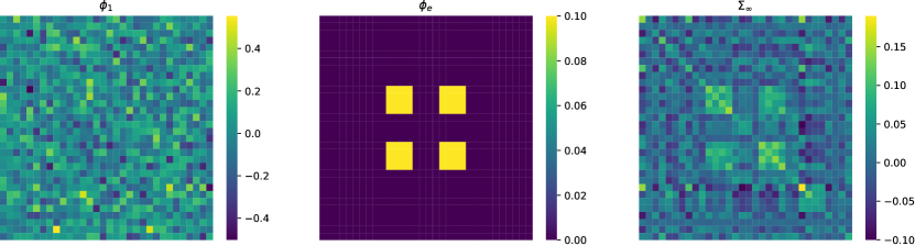
\displaystyle X_{t+1}=\phi_{1}\cos(X_{t}^{\top}X_{t-2}X_{t}^{\top})+\phi_{2}\sqrt{\max\{0,X_{t-1}^{\top}\}}+\phi_{e}E_{t+1}.

Here $X_{t}\in\mathbb{R}^{p_{1}\times p_{2}}$ and $E_{t+1}\in\mathbb{R}^{p_{1}\times p_{2}}$ represent target image and independent noise matrices, respectively, with the image size fixed to be $(p_{1},p_{2})=(32,32)$ . In all three cases, we let the noise matrix $E_{t+1}$ consists of i.i.d. standard normal entries. Moreover, the initialization $X_{0}$ in Cases 1 and 2 and $X_{0}$ , $X_{1}$ , and $X_{2}$ in Case 3 are also taken to the matrices with i.i.d. standard normal entries. It is worth noting that under Case 1 setting, $X_{t}$ is column-wise independent, and each column of $X_{t}$ converges to ${\cal N}(0,\Sigma_{\infty})$ , where $\Sigma_{\infty}$ satisfies $\Sigma_{\infty}=\phi_{1}\Sigma_{\infty}\phi_{1}^{\top}+\phi_{e}\phi_{e}^{\top}$ . In this simulation, we let $\phi_{1}\in\mathbb{R}^{32\times 32}$ be a normalized Gaussian matrix with the largest eigenvalue modulus less than 1, $\phi_{e}\in\mathbb{R}^{32\times 32}$ is a fixed matrix with block shape patterns. Given $\phi_{1}$ and $\phi_{e}$ , then $\Sigma_{\infty}$ could be solved easily. We plot the $\phi_{1}$ , $\phi_{e}$ and $\Sigma_{\infty}$ in the supplementary material. Moreover, in Case 2, we set $\phi_{1}$ , $\phi_{e}\in\mathbb{R}^{32\times 32}$ in a similar manner as Case 1, but certainly, the normal convergence would no longer hold. While in Case 3, we let both $\phi_{1}$ and $\phi_{2}\in\mathbb{R}^{32\times 32}$ be normalized Gaussian matrices, and fix $\phi_{e}\in\mathbb{R}^{32\times 32}$ as before.

We consider the time series with two different lengths, $T=1000$ and $T=5000$ for training. We set the horizon $S=3$ , i.e., generate images in a maximum of $S=3$ steps. We aim to generate a total of $T_{new}=500$ image points in a “rolling forecasting” style. Specifically, for any $s=1,\ldots,D$ , we let the $s$ -step generation (denoted as “s-step GTS”) be

\displaystyle{\widetilde{X}}_{T+t_{new}}^{(j)}(s)=\widehat{G}\left(X_{T+t_{new}-s},\eta^{(j)}_{T+t_{new}-s},s\right),

where $t_{new}\leq T_{new}$ and superscript $j$ indicting the j-th generation. Here $\widehat{G}$ is estimated using 10,000 randomly selected pairs $(X_{t},X_{t+s})$ from the training data. While for iteration generation (denoted as “iter GTS”), we let

\displaystyle\widehat{X}_{T+t_{new}}^{(j)}(s)=\widehat{g}^{(s)}\left(X_{T+t_{new}-s},[\eta^{(j)}_{T+t_{new}-s},\ldots,\eta^{(j)}_{T+t_{new}-1}]\right),

where $\widehat{g}^{(s)}$ is the $s$ -times composition of the function $\widehat{g}$ .

The $\widehat{G}$ for s-step generation (and $\widehat{g}$ for iterative generation) are estimated for KL divergence (i.e., $f(x)=x\log x$ ) using neural networks in the simulation. Specifically, in Case 1 and 2, the input $X_{t}$ initially goes through two fully connected layers, each with ReLU activation functions. Afterward, it is combined with the random noise vector $\eta$ . This combined input is then passed through a single fully connected layer. The discriminator has two separate processing branches that embed $X_{t}$ and $X_{t+1}$ into low-dimensional vectors, respectively. These vectors are concatenated and further processed to produce an output score. The details of network structure can be found in Table 1. While for Case 3, in the generator network, $X_{t}$ , $X_{t-1}$ , and $X_{t-2}$ are each processed independently using three separate fully-connected layers. Afterward, they are combined with a random noise vector and passed through another fully-connected layer before producing the output. The discriminator in this case follows the same process as in Cases 1 and 2.

Different from supervised learning, generative learning does not have universally applicable metrics for evaluating the quality of generated samples (Theis et al.,, 2015; Borji,, 2022). Assessing the visual quality of produced images often depends on expert domain knowledge. Meanwhile, the GANs literature has seen significant efforts in understanding and developing evaluation metrics for generative performance. Several quantitative metrics have been introduced, such as Inception Score (Salimans et al.,, 2016), Frechet Inception Distance (Heusel et al.,, 2017), and Maximum Mean Discrepancy (Bińkowski et al.,, 2018), among others.

Table 1: The architecture of generator and discriminator for case 1 and 2.

	Layer	Type
	1	fully connected layer (in dims = 1024, out dims = 256)
	2	ReLU
generator	3	fully connected layer (in dims = 256, out dims = 128)
	4	ReLU
	5	concatenate with random vector $\eta$
	6	fully connected layer (in dims = 148, out dims = 1024)
discriminator	$\left.\begin{matrix}X_{t}\xrightarrow{\text{fc+ReLU}}64\xrightarrow{\text{fc}}x_{t}\in{\mathbb{R}}^{64}\\ X_{t+1}\xrightarrow{\text{fc+ReLU }}x_{t+1}\in{\mathbb{R}}^{64}\end{matrix}\right\}\text{concatenate}(x_{t},x_{t+1})\xrightarrow{\text{fc+ReLU}}64\xrightarrow{\text{fc }}\text{score}$

Table 2: The NRMSE of mean estimation in Study I under different settings. The best and second best results are marked by green and bold respectively.

$T$	Cases	Methods	$s=1$	$s=2$	$s=3$
		OLS	${\color[rgb]{0.0,0.47,0.44}\bf{0.013}}$ (0.002)	${\color[rgb]{0.0,0.47,0.44}\bf{0.017}}$ (0.003)	${\color[rgb]{0.0,0.47,0.44}\bf{0.023}}$ (0.004)
	case 1	Naive Baseline	1.563 (0.039)	1.932 (0.043)	1.408 (0.098)
		iter GTS	$\bf{0.800}$ (0.038)	0.891 (0.050)	0.985 (0.064)
		s-step GTS	$\bf{0.800}$ (0.038)	$\bf{0.843}$ (0.047)	$\bf{0.966}$ (0.062)
		OLS	0.973 (0.060)	1.000 (0.021)	0.995 (0.008)
1000	case 2	Naive Baseline	1.462 (0.129)	1.455 (0.152)	1.373 (0.178)
		iter GTS	${\color[rgb]{0.0,0.47,0.44}\bf{0.606}}$ (0.053)	$\bf{0.664}$ (0.064)	$\bf{0.702}$ (0.075)
		s-step GTS	${\color[rgb]{0.0,0.47,0.44}\bf{0.606}}$ (0.053)	${\color[rgb]{0.0,0.47,0.44}\bf{0.609}}$ (0.057)	${\color[rgb]{0.0,0.47,0.44}\bf{0.615}}$ (0.061)
		OLS	0.608 (0.021)	0.609 (0.021)	0.609 (0.020)
	case 3	Naive Baseline	0.845 (0.034)	0.843 (0.034)	0.844 (0.033)
		iter GTS	${\color[rgb]{0.0,0.47,0.44}\bf{0.598}}$ (0.020)	${\color[rgb]{0.0,0.47,0.44}\bf{0.595}}$ (0.020)	${\color[rgb]{0.0,0.47,0.44}\bf{0.598}}$ (0.020)
		s-step GTS	${\color[rgb]{0.0,0.47,0.44}\bf{0.598}}$ (0.020)	${\color[rgb]{0.0,0.47,0.44}\bf{0.595}}$ (0.020)	$\bf{0.602}$ (0.020)
		OLS	${\color[rgb]{0.0,0.47,0.44}\bf{0.007}}$ (0.001)	${\color[rgb]{0.0,0.47,0.44}\bf{0.010}}$ (0.002)	${\color[rgb]{0.0,0.47,0.44}\bf{0.013}}$ (0.002)
	case 1	Naive Baseline	1.563 (0.040)	1.932 (0.043)	1.408 (0.099)
		iter GTS	$\bf{0.615}$ (0.098)	0.717 (0.163)	0.851 (0.226)
		s-step GTS	$\bf{0.615}$ (0.098)	$\bf{0.707}$ (0.167)	$\bf{0.749}$ (0.079)
		OLS	0.973 (0.060)	1.001 (0.021)	0.995 (0.007)
5000	case 2	Naive Baseline	1.468 (0.132)	1.452 (0.157)	1.377 (0.181)
		iter GTS	${\color[rgb]{0.0,0.47,0.44}\bf{0.470}}$ (0.046)	$\bf{0.532}$ (0.056)	$\bf{0.576}$ (0.066)
		s-step GTS	${\color[rgb]{0.0,0.47,0.44}\bf{0.470}}$ (0.046)	${\color[rgb]{0.0,0.47,0.44}\bf{0.470}}$ (0.048)	${\color[rgb]{0.0,0.47,0.44}\bf{0.500}}$ (0.054)
		OLS	0.608 (0.020)	0.610 (0.021)	0.609 (0.020)
	case 3	Naive Baseline	0.845 (0.032)	0.846 (0.032)	0.850 (0.033)
		iter GTS	${\color[rgb]{0.0,0.47,0.44}\bf{0.578}}$ (0.020)	$\bf{0.574}$ (0.020)	$\bf{0.595}$ (0.020)
		s-step GTS	${\color[rgb]{0.0,0.47,0.44}\bf{0.578}}$ (0.020)	${\color[rgb]{0.0,0.47,0.44}\bf{0.566}}$ (0.020)	${\color[rgb]{0.0,0.47,0.44}\bf{0.592}}$ (0.021)

Nonetheless, achieving a consensus regarding the evaluation of generative models remains an unresolved issue. In our approach, we compute the mean of the generated samples and present the results as the normalized root mean squared error (NRMSE) of the mean estimation. Specifically, for a given step $s$ , let ${\widetilde{X}}_{T+t_{new}}(s)=(1/J)\sum_{j=1}^{J}{\widetilde{X}}_{T+t_{new}}^{(j)}(s)$ and $\widehat{X}_{T+t_{new}}(s)=(1/J)\sum_{j=1}^{J}\widehat{X}_{T+t_{new}}^{(j)}(s)$ be the estimated mean of the s-step and iterative generated samples, respectively. The NRMSE of the iterative generation is defined as

\displaystyle\text{NRMSE}(s)=\|\widehat{X}_{T+t_{new}}(s)-{\mathbb{E}}X_{T+t_{new}}\|_{F}/\|{\mathbb{E}}X_{T+t_{new}}\|_{F},

where $\|\cdot\|_{F}$ denotes the Frobenius norm. The NRMSE of the s-step generation can be defined similarly.

The performance of our iterative and s-step generation are compared with two benchmark approaches. We first consider a naive baseline in which the prediction for $X_{T+t_{new}}$ is taken from the observation $s$ -steps ahead for a given $s=1,\ldots,S$ , meaning that $\widehat{X}_{T+t_{new}}=X_{T+t_{new}-s}$ . In addition, we consider a simple linear estimator obtained using Ordinary Least Squares (OLS). Specifically, the linear coefficients are estimated with a correctly specified order of lag, i.e., $\widehat{\phi}_{1}=\mathop{\rm arg\,min}_{\phi}\sum_{t=1}^{T}\|X_{t+1}-\phi X_{t}\|_{F}$ for Cases 1 and 2, and $(\widehat{\phi}_{1},\widehat{\phi}_{2},\widehat{\phi}_{3})=\mathop{\rm arg\,min}_{\phi_{1},\phi_{2},\phi_{3}}\sum_{t=1}^{T}\|X_{t+1}-\phi_{1}X_{t}-\phi_{2}X_{t-1}-\phi_{3}X_{t-2}\|_{F}$ for Case 3. Clearly, in Case 1, OLS is a suitable choice as the model is linear. However, for Cases 2 and 3, OLS is mis-specified.

We repeat the simulation for 100 times and report in Table 2 the mean and standard deviation of the NRMSE for $s=1,2,3$ using different approaches. It is clear that our s-step and iterative generations exhibit competitive performance across almost all settings, particularly in the nonlinear Cases 2 and 3. In Case 1, the original model is linear, and as expected, OLS achieves the minimum NRMSE. Moreover, as $s$ increases, the problem becomes more challenging. However, both s-step and iterative generation maintain robust performance across different $s$ . It is important to note that when $s=1$ , the iterative and s-step generation methods are equivalent. For $s=2,3$ , the s-step generation generally exhibits a slightly smaller NRMSE, though the difference is not significant.

6.2 Study II: Multiple Time Series

In this subsection, we consider a panel data setting with multiple time series. We consider two different sample sizes, $n=200,500$ while fixing the time series length $T=20$ . We set the horizon $S=3$ as before, i.e., generate images in a maximum of $S=3$ steps for each subject.

Table 3: The NRMSE of mean estimation in Study II under different settings. The best and second best results are marked by green and bold respectively.

$(n,T)$	Cases	Methods	$s=1$	$s=2$	$s=3$
		OLS	${\color[rgb]{0.0,0.47,0.44}\bf{0.037}}$ (0.001)	${\color[rgb]{0.0,0.47,0.44}\bf{0.070}}$ (0.002)	${\color[rgb]{0.0,0.47,0.44}\bf{0.096}}$ (0.003)
	case 1	Naive Baseline	1.563 (0.039)	1.925 (0.043)	1.380 (0.097)
		iter GTS	$\bf{0.729}$ (0.036)	0.813 (0.046)	0.893 (0.056)
		s-step GTS	$\bf{0.729}$ (0.036)	$\bf{0.780}$ (0.044)	$\bf{0.885}$ (0.056)
		OLS	0.985 (0.029)	1.000 (0.005)	0.999 (0.001)
$(200,20)$	case 2	Naive Baseline	1.459 (0.107)	1.478 (0.127)	1.415 (0.156)
		iter GTS	${\color[rgb]{0.0,0.47,0.44}\bf{0.583}}$ (0.049)	${\color[rgb]{0.0,0.47,0.44}\bf{0.647}}$ (0.060)	${\color[rgb]{0.0,0.47,0.44}\bf{0.690}}$ (0.071)
		s-step GTS	${\color[rgb]{0.0,0.47,0.44}\bf{0.583}}$ (0.049)	$\bf{0.689}$ (0.068)	$\bf{0.710}$ (0.077)
		OLS	0.617 (0.018)	0.620 (0.018)	0.625 (0.015)
	case 3	Naive Baseline	0.847 (0.032)	0.845 (0.033)	0.846 (0.034)
		iter GTS	${\color[rgb]{0.0,0.47,0.44}\bf{0.593}}$ (0.019)	${\color[rgb]{0.0,0.47,0.44}\bf{0.590}}$ (0.020)	${\color[rgb]{0.0,0.47,0.44}\bf{0.594}}$ (0.020)
		s-step GTS	${\color[rgb]{0.0,0.47,0.44}\bf{0.593}}$ (0.019)	$\bf{0.592}$ (0.020)	$\bf{0.597}$ (0.020)
		OLS	${\color[rgb]{0.0,0.47,0.44}\bf{0.037}}$ (0.001)	${\color[rgb]{0.0,0.47,0.44}\bf{0.069}}$ (0.002)	${\color[rgb]{0.0,0.47,0.44}\bf{0.096}}$ (0.003)
	case 1	Naive Baseline	1.564 (0.039)	1.925 (0.043)	1.379 (0.098)
		iter GTS	$\bf{0.611}$ (0.040)	0.667 (0.053)	$\bf{0.755}$ (0.072)
		s-step GTS	$\bf{0.611}$ (0.040)	$\bf{0.647}$ (0.066)	0.763 (0.056)
		OLS	0.985 (0.029)	1.000 (0.005)	0.999 (0.001)
$(500,20)$	case 2	Naive Baseline	1.458 (0.109)	1.478 (0.128)	1.414 (0.156)
		iter GTS	${\color[rgb]{0.0,0.47,0.44}\bf{0.511}}$ (0.050)	${\color[rgb]{0.0,0.47,0.44}\bf{0.578}}$ (0.060)	${\color[rgb]{0.0,0.47,0.44}\bf{0.625}}$ (0.070)
		s-step GTS	${\color[rgb]{0.0,0.47,0.44}\bf{0.511}}$ (0.050)	$\bf{0.639}$ (0.069)	$\bf{0.682}$ (0.080)
		OLS	0.617 (0.018)	0.619 (0.018)	0.625 (0.015)
	case 3	Naive Baseline	0.847 (0.032)	0.845 (0.033)	0.846 (0.034)
		iter GTS	${\color[rgb]{0.0,0.47,0.44}\bf{0.579}}$ (0.019)	${\color[rgb]{0.0,0.47,0.44}\bf{0.577}}$ (0.020)	${\color[rgb]{0.0,0.47,0.44}\bf{0.592}}$ (0.020)
		s-step GTS	${\color[rgb]{0.0,0.47,0.44}\bf{0.579}}$ (0.019)	$\bf{0.579}$ (0.020)	$\bf{0.593}$ (0.021)

Analogous to the single time series, we repeat the simulation for 100 times and report in Table 3 the mean and standard deviation of the NRMSE for $s=1,2,3$ using different approaches. Table 3 shows a similar pattern as Table 2. Both iterative and s-step generated images achieve the minimum NRMSE in Case 2 and 3. While under the linear Case 1, the OLS continues to achieve the lowest NRMSE. One notable difference in Table 3 is that the iterative generation achieves a lower NRMSE compared to the s-step generation in this case. One potential explanation for this is the increase in sample size. In comparison to the single time series setting, a sample size of $n=200$ or $500$ allows the iterative approach to obtain a better $g$ estimation, which in turn enhances the image generation process.

7 The ADNI study

Driven by the goal of understanding the brain aging process, we in this section study real brain MRI data from the Alzheimer’s Disease Neuroimaging Initiative (ADNI). Introduced by Petersen et al., (2010), ADNI aims to investigate the progression of Alzheimer’s disease (AD) by collecting sequential MRI scans of subjects classified as cognitively normal (CN), mildly cognitively impaired (MCI), and those with AD.

Our study focuses on analyzing the brain’s progression during the MCI stage. We include a total of 565 participants from the MCI group in our analysis, each having a sequence of T1-weighted MRI scans with lengths varying between 3 and 9. We approach this as an imaging time series generation problem with multiple samples. However, a significant challenge with the dataset is the short length of each sample ( $T_{i}\leq 9$ ), a common issue in brain imaging analysis. Given the short length of these samples, we do not generate new images beyond a specific point $T$ , as it would be difficult to evaluate their quality. Instead, we divide the dataset into a training set consisting of 450 samples and a testing set comprising 115 samples. We then train the generator $G$ using the training set and generate image sequences for the testing set given the starting point $X_{0}$ . As in the simulation study, we also consider a naive baseline in which the prediction for $X_{i,s}$ is taken from the observation $s$ -steps ahead, meaning that $\widehat{X}_{i,s}=X_{i,0}$ . It is worth mentioning that OLS is not suitable for MRI analysis and, as such, is not included in this context.

In our study, all brain T1-weighted MRI scans are processed through a standard pipeline which begins with a spatial adaptive non-local means (SANLM) denoising filter (Manjón et al.,, 2010), then followed by resampling, bias-correction, affine-registration and unified segmentation (Ashburner and Friston,, 2005), skull-stripping and cerebellum removing. Each MRI is then locally intensity corrected and spatially normalized into the Montreal Neurological Institute (MNI) atlas space (Ashburner,, 2007). These procedures result in processed images of size $169\times 205\times 169$ . We further rescale the intensities of the resulting images to a range of $[-1,1]$ . We select the central axial slice from each MRI and crop it to a size of $144\times 192$ by removing the zero-valued voxels.

Figure 1 plots the original, iterative and s-step generated MRI sequence along with their difference to $X_{0}$ for one subject in the test set. As shown by the original images, the brain changes gradually as age increases. This pattern is clearly captured by both iterative and s-step generations. To further assess the generated MRI images, we plot the starting image $X_{0}$ , true image after s step (i.e., $X_{s}$ ), iteratively and $s$ -step generated images (i.e., $\widehat{X}_{s}$ and ${\widetilde{X}}_{s}$ ) for three subjects in Figure 2.

\begin{overpic}[width=433.62pt]{real_fig_sequences.pdf} \put(88.0,42.0){$X_{s}-X_{0}$} \put(88.0,36.0){$X_{s}$} \par\put(88.0,27.0){$\widehat{X}_{s}-X_{0}$} \put(88.0,21.0){$\widehat{X}_{s}$} \par\put(88.0,12.0){${\widetilde{X}}_{s}-X_{0}$} \put(88.0,6.0){${\widetilde{X}}_{s}$} \par\end{overpic}

Figure 1: The original, iterative and s-step generated MRI sequence

s=0,1,\ldots,7

along with their difference to

X_{0}

for one subject.

Although the differences are subtle, we can observe that the image $X_{s}$ and the generated images, $\widehat{X}_{s}$ and ${\widetilde{X}}_{s}$ , are quite similar, but they all deviate from $X_{0}$ in several crucial regions. We highlight four of these regions in Figure 2, including: a) cortical sulci, b) ventricles, c) edge of ventricles, and d) anterior inter-hemispheric fissure. More specifically, we can observe (from subjects 1, 2, and 3, region a) that the cortical sulci widen as age increases. The widening of cortical sulci may be associated with white matter degradation (Drayer,, 1988; Walhovd et al.,, 2005). This phenomenon is also observed in patients with Alzheimer’s Disease (Migliaccio et al.,, 2012). Additionally, the brain ventricles expand from time $0$ to $s$ as suggested by subjects 1 and 3, region b. The enlargement of ventricles during the aging process is one of the most striking features in structural brain scans across the lifespan (MacDonald and Pike,, 2021). Moreover, we notice that the edge of the ventricles becomes softer (darker region of subject 1, region c), and there is an increased presence of low signal areas adjacent to the ventricles (subject 2, regions b and c). From a clinical perspective, this observation suggests the existence of periventricular interstitial edema, which is linked to reduced ependyma activity and brain white matter atrophy (Todd et al.,, 2018). Lastly, the anterior interhemispheric fissure deepens with aging, as demonstrated in subject 1, region d. In conclusion, the generated samples can potentially aid clinical analyses in identifying age-related brain issues.

\begin{overpic}[width=433.62pt]{real_fig_subjects.pdf} \put(18.0,50.0){$X_{0}$ (age 71)} \put(38.0,50.0){$X_{s}$ (age 80)} \put(61.0,50.0){iterative} \put(82.0,50.0){s-step} \put(18.0,25.5){$X_{0}$ (age 72)} \put(38.0,25.5){$X_{s}$ (age 78)} \put(61.0,25.5){iterative} \put(82.0,25.5){s-step} \put(18.0,1.5){$X_{0}$ (age 72)} \put(38.0,1.5){$X_{s}$ (age 77)} \put(61.0,1.5){iterative} \put(82.0,1.5){s-step} \end{overpic}

Figure 2: An illustration of the generated samples for three subjects in the testing group. For each subject, we present from left to right: starting image

X_{0}

, target

X_{s}

, and two generated samples

\widehat{X}_{s}

and

{\widetilde{X}}_{s}

by iterative and s-step generation respectively. Moreover, we highlight (with different colors) four different regions that

X_{s}

(along with

\widehat{X}_{s}

and

{\widetilde{X}}_{s}

) are most different from

X_{0}

, including: a) cortical sulci, b) ventricles, c) edge of ventricles, d) anterior interhemispheric fissure.

As discussed before, there is a lack of universally application metric for evaluating the quality of generated images. In this study, we consider three metrics to measure the difference between the target $X_{s}$ and our generations $\widehat{X}_{s}$ : structural similarity index measure (SSIM), peak signal-to-noise ratio (PSNR), along with the previously introduced NRMSE. More specifically, SSIM calculates the similarity score between two images by comparing their luminance, contrast, and structure. Given two images $X$ and $Y$ , it is defined as

\displaystyle\text{SSIM}(X,Y)=\frac{(2\mu_{x}\mu_{y}+c_{1})(2\sigma_{xy}+c_{2})}{(\mu_{x}^{2}+\mu_{y}^{2}+c_{1})(\sigma_{x}^{2}+\sigma_{y}^{2}+c_{2})},

where $(\mu_{x},\mu_{y})$ , $(\sigma_{x}^{2},\sigma_{y}^{2})$ are the mean and variance of pixel values in $X$ and $Y$ respectively. The $\sigma_{xy}$ is the covariance of $X$ and $Y$ and $c_{1}$ , $c_{2}$ are constants, to be specified in the supplementary material. PSNR is a widely used engineering term for measuring the reconstruction quality for images subject to lossy compression. It is typically defined using the mean squared error:

\displaystyle\text{PSNR}(X,Y)=10\log_{10}\left(c^{2}/\text{MSE}(X,Y)\right),

where $c$ is the maximum pixel value among $X,Y$ and $\text{MSE}(X,Y)=\|X-Y\|_{F}^{2}/(D_{1}D_{2})$ . Clearly, better image generation performance is indicated by higher values of SSIM and PSNR, as well as smaller values of NRMSE.

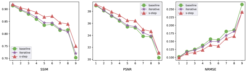
In Figure 3, we present for each $s$ the mean SSIM, PSNR, and NRMSE over all subjects in the testing set. The results clearly indicate that both s-step and iterative generations outperform the benchmark in all three metrics across almost all the $s=1,\ldots,9$ , providing strong evidence of the high quality of our generated images. As $s$ increases, the generation problem becomes more challenging. Consequently, we observe a decrease in both SSIM and PSNR for both iterative and s-step generations, indicating a decline in generation quality. On the other hand, the NRMSE for both approaches increase, suggesting a higher level of error in the generated images. When further comparing the iterative and s-step generation, the s-step generation shows a dominating performance in this study. The major reason is due to the limited sample size. With fewer than 500 subjects in training and the observed sequence for each subject being less than 9, a direct s-step generation approach proves advantageous compared to the iterative generation method.

Refer to caption — Figure 3: The mean SSIM, PSNR, and NRMSE over all testing subjects in the ADNI data analysis for $s=1,\ldots,9$ .

In summary, this study further validates the effectiveness of our approach in generating image sequences. Incorporating the generated image sequences as data augmentation (Chen et al., 2022c, ) could further enhance the performance of downstream tasks, such as Alzheimer’s disease detection (Xia et al.,, 2022). As mentioned before, AD is the most prevalent neurodegenerative disorder, progressively leading to irreversible neuronal damage. The early diagnosis of AD and its syndromes, such as MCI, is of significant importance. We believe that the proposed image time series learning offers valuable assistance in understanding and identifying AD, as well as other aging-related brain issues.

References

Anthony and Bartlett, (1999) Anthony, M. and Bartlett, P. L. (1999). Neural Network Learning: Theoretical Foundations. Cambridge University Press.
Ashburner, (2007) Ashburner, J. (2007). A fast diffeomorphic image registration algorithm. Neuroimage, 38(1):95–113.
Ashburner and Friston, (2005) Ashburner, J. and Friston, K. J. (2005). Unified segmentation. Neuroimage, 26(3):839–851.
Bartlett et al., (2017) Bartlett, P. L., Harvey, N., Liaw, C., and Mehrabian, A. (2017). Nearly-tight vc-dimension and pseudodimension bounds for piecewise linear neural networks.
Basu and Michailidis, (2015) Basu, S. and Michailidis, G. (2015). Regularized estimation in sparse high-dimensional time series models.
Bauer and Kohler, (2019) Bauer, B. and Kohler, M. (2019). On deep learning as a remedy for the curse of dimensionality in nonparametric regression.
Bińkowski et al., (2018) Bińkowski, M., Sutherland, D. J., Arbel, M., and Gretton, A. (2018). Demystifying mmd gans. arXiv preprint arXiv:1801.01401.
Bollerslev, (1986) Bollerslev, T. (1986). Generalized autoregressive conditional heteroskedasticity. Journal of econometrics, 31(3):307–327.
Borji, (2022) Borji, A. (2022). Pros and cons of gan evaluation measures: New developments. Computer Vision and Image Understanding, 215:103329.
Brockwell and Davis, (1991) Brockwell, P. J. and Davis, R. A. (1991). Time series: theory and methods. Springer science & business media.
Chang et al., (2023) Chang, J., He, J., Yang, L., and Yao, Q. (2023). Modelling matrix time series via a tensor cp-decomposition. Journal of the Royal Statistical Society Series B: Statistical Methodology, 85(1):127–148.
Chen et al., (2021) Chen, R., Xiao, H., and Yang, D. (2021). Autoregressive models for matrix-valued time series. Journal of Econometrics, 222(1):539–560.
(13) Chen, R., Yang, D., and Zhang, C.-H. (2022a). Factor models for high-dimensional tensor time series. Journal of the American Statistical Association, 117(537):94–116.
(14) Chen, Y., Gao, Q., and Wang, X. (2022b). Inferential wasserstein generative adversarial networks. Journal of the Royal Statistical Society Series B: Statistical Methodology, 84(1):83–113.
(15) Chen, Y., Yang, X.-H., Wei, Z., Heidari, A. A., Zheng, N., Li, Z., Chen, H., Hu, H., Zhou, Q., and Guan, Q. (2022c). Generative adversarial networks in medical image augmentation: a review. Computers in Biology and Medicine, 144:105382.
Cole et al., (2018) Cole, J. H., Ritchie, S. J., Bastin, M. E., Hernández, V., Muñoz Maniega, S., Royle, N., Corley, J., Pattie, A., Harris, S. E., Zhang, Q., et al. (2018). Brain age predicts mortality. Molecular psychiatry, 23(5):1385–1392.
Drayer, (1988) Drayer, B. P. (1988). Imaging of the aging brain. part i. normal findings. Radiology, 166(3):785–796.
Engle, (1982) Engle, R. F. (1982). Autoregressive conditional heteroscedasticity with estimates of the variance of united kingdom inflation. Econometrica: Journal of the econometric society, pages 987–1007.
Fan and Yao, (2003) Fan, J. and Yao, Q. (2003). Nonlinear time series: nonparametric and parametric methods, volume 20. Springer.
Feng and Yang, (2023) Feng, L. and Yang, G. (2023). Deep kronecker network. Biometrika, page asad049.
Feng et al., (2019) Feng, X., Li, T., Song, X., and Zhu, H. (2019). Bayesian scalar on image regression with nonignorable nonresponse. Journal of the American Statistical Association, pages 1–24.
Goodfellow et al., (2014) Goodfellow, I., Pouget-Abadie, J., Mirza, M., Xu, B., Warde-Farley, D., Ozair, S., Courville, A., and Bengio, Y. (2014). Generative adversarial nets. Advances in neural information processing systems, 27.
Guo et al., (2016) Guo, S., Wang, Y., and Yao, Q. (2016). High-dimensional and banded vector autoregressions. Biometrika, page asw046.
Han et al., (2023) Han, Y., Chen, R., Zhang, C.-H., and Yao, Q. (2023). Simultaneous decorrelation of matrix time series. Journal of the American Statistical Association, pages 1–13.
Heusel et al., (2017) Heusel, M., Ramsauer, H., Unterthiner, T., Nessler, B., and Hochreiter, S. (2017). Gans trained by a two time-scale update rule converge to a local nash equilibrium. Advances in neural information processing systems, 30.
Ho et al., (2020) Ho, J., Jain, A., and Abbeel, P. (2020). Denoising diffusion probabilistic models. Advances in neural information processing systems, 33:6840–6851.
Huizinga et al., (2018) Huizinga, W., Poot, D. H., Vernooij, M. W., Roshchupkin, G. V., Bron, E. E., Ikram, M. A., Rueckert, D., Niessen, W. J., Klein, S., Initiative, A. D. N., et al. (2018). A spatio-temporal reference model of the aging brain. NeuroImage, 169:11–22.
Jack et al., (2004) Jack, C., Shiung, M., Gunter, J., O’brien, P., Weigand, S., Knopman, D. S., Boeve, B. F., Ivnik, R. J., Smith, G. E., Cha, R., et al. (2004). Comparison of different mri brain atrophy rate measures with clinical disease progression in ad. Neurology, 62(4):591–600.
Jiao et al., (2021) Jiao, Y., Shen, G., Lin, Y., and Huang, J. (2021). Deep nonparametric regression on approximately low-dimensional manifolds. arXiv preprint arXiv:2104.06708.
Kallenberg, (2021) Kallenberg, O. (2021). Foundations of modern probability. Probability Theory and Stochastic Modelling.
Kang et al., (2018) Kang, J., Reich, B. J., and Staicu, A.-M. (2018). Scalar-on-image regression via the soft-thresholded gaussian process. Biometrika, 105(1):165–184.
Keziou, (2003) Keziou, A. (2003). Dual representation of $\varphi$ -divergences and applications. Comptes rendus mathématique, 336(10):857–862.
Kingma and Welling, (2013) Kingma, D. P. and Welling, M. (2013). Auto-encoding variational bayes. arXiv preprint arXiv:1312.6114.
Lai et al., (2018) Lai, G., Chang, W.-C., Yang, Y., and Liu, H. (2018). Modeling long-and short-term temporal patterns with deep neural networks. In The 41st international ACM SIGIR conference on research & development in information retrieval, pages 95–104.
LeCun et al., (1998) LeCun, Y., Bottou, L., Bengio, Y., and Haffner, P. (1998). Gradient-based learning applied to document recognition. Proceedings of the IEEE, 86(11):2278–2324.
Li et al., (2019) Li, S., Jin, X., Xuan, Y., Zhou, X., Chen, W., Wang, Y.-X., and Yan, X. (2019). Enhancing the locality and breaking the memory bottleneck of transformer on time series forecasting. Advances in neural information processing systems, 32.
Li et al., (2018) Li, X., Xu, D., Zhou, H., and Li, L. (2018). Tucker tensor regression and neuroimaging analysis. Statistics in Biosciences, 10(3):520–545.
Loshchilov and Hutter, (2017) Loshchilov, I. and Hutter, F. (2017). Decoupled weight decay regularization. arXiv preprint arXiv:1711.05101.
Lu et al., (2020) Lu, J., Shen, Z., Yang, H., and Zhang, S. (2020). Deep network approximation for smooth functions. arxiv e-prints, page. arXiv preprint arXiv:2001.03040.
Luo and Zhang, (2023) Luo, Y. and Zhang, A. R. (2023). Low-rank tensor estimation via riemannian gauss-newton: Statistical optimality and second-order convergence. The Journal of Machine Learning Research, 24(1):18274–18321.
MacDonald and Pike, (2021) MacDonald, M. E. and Pike, G. B. (2021). Mri of healthy brain aging: A review. NMR in Biomedicine, 34(9):e4564.
Manjón et al., (2010) Manjón, J. V., Coupé, P., Martí-Bonmatí, L., Collins, D. L., and Robles, M. (2010). Adaptive non-local means denoising of mr images with spatially varying noise levels. Journal of Magnetic Resonance Imaging, 31(1):192–203.
McDonald and Shalizi, (2017) McDonald, D. J. and Shalizi, C. R. (2017). Rademacher complexity of stationary sequences.
Migliaccio et al., (2012) Migliaccio, R., Agosta, F., Possin, K. L., Rabinovici, G. D., Miller, B. L., and Gorno-Tempini, M. L. (2012). White matter atrophy in alzheimer’s disease variants. Alzheimer’s & Dementia, 8:S78–S87.
Nguyen et al., (2010) Nguyen, X., Wainwright, M. J., and Jordan, M. I. (2010). Estimating divergence functionals and the likelihood ratio by convex risk minimization. IEEE Transactions on Information Theory, 56(11):5847–5861.
Nowozin et al., (2016) Nowozin, S., Cseke, B., and Tomioka, R. (2016). f-gan: Training generative neural samplers using variational divergence minimization. Advances in neural information processing systems, 29.
Pascanu et al., (2013) Pascanu, R., Gulcehre, C., Cho, K., and Bengio, Y. (2013). How to construct deep recurrent neural networks. arXiv preprint arXiv:1312.6026.
Petersen et al., (2010) Petersen, R. C., Aisen, P. S., Beckett, L. A., Donohue, M. C., Gamst, A. C., Harvey, D. J., Jack, C. R., Jagust, W. J., Shaw, L. M., Toga, A. W., et al. (2010). Alzheimer’s disease neuroimaging initiative (adni): clinical characterization. Neurology, 74(3):201–209.
Ravi et al., (2019) Ravi, D., Alexander, D. C., Oxtoby, N. P., and Initiative, A. D. N. (2019). Degenerative adversarial neuroimage nets: generating images that mimic disease progression. In International Conference on Medical Image Computing and Computer-Assisted Intervention, pages 164–172. Springer.
Salimans et al., (2016) Salimans, T., Goodfellow, I., Zaremba, W., Cheung, V., Radford, A., and Chen, X. (2016). Improved techniques for training gans. Advances in neural information processing systems, 29.
Schmidt-Hieber, (2020) Schmidt-Hieber, J. (2020). Nonparametric regression using deep neural networks with relu activation function.
Shen et al., (2021) Shen, G., Jiao, Y., Lin, Y., Horowitz, J. L., and Huang, J. (2021). Deep quantile regression: Mitigating the curse of dimensionality through composition. arXiv preprint arXiv:2107.04907.
Shen et al., (2019) Shen, Z., Yang, H., and Zhang, S. (2019). Deep network approximation characterized by number of neurons. arXiv preprint arXiv:1906.05497.
Stock and Watson, (2001) Stock, J. H. and Watson, M. W. (2001). Vector autoregressions. Journal of Economic perspectives, 15(4):101–115.
Stone, (1982) Stone, C. J. (1982). Optimal global rates of convergence for nonparametric regression. The annals of statistics, pages 1040–1053.
Theis et al., (2015) Theis, L., Oord, A. v. d., and Bethge, M. (2015). A note on the evaluation of generative models. arXiv preprint arXiv:1511.01844.
Tibshirani, (1996) Tibshirani, R. (1996). Regression shrinkage and selection via the lasso. Journal of the Royal Statistical Society. Series B (Methodological), pages 267–288.
Todd et al., (2018) Todd, K. L., Brighton, T., Norton, E. S., Schick, S., Elkins, W., Pletnikova, O., Fortinsky, R. H., Troncoso, J. C., Molfese, P. J., Resnick, S. M., et al. (2018). Ventricular and periventricular anomalies in the aging and cognitively impaired brain. Frontiers in aging neuroscience, 9:445.
Tofts, (2005) Tofts, P. (2005). Quantitative MRI of the brain: measuring changes caused by disease. John Wiley & Sons.
Tsay, (2013) Tsay, R. S. (2013). Multivariate time series analysis: with R and financial applications. John Wiley & Sons.
Tsay and Chen, (2018) Tsay, R. S. and Chen, R. (2018). Nonlinear time series analysis, volume 891. John Wiley & Sons.
Walhovd et al., (2005) Walhovd, K. B., Fjell, A. M., Reinvang, I., Lundervold, A., Dale, A. M., Eilertsen, D. E., Quinn, B. T., Salat, D., Makris, N., and Fischl, B. (2005). Effects of age on volumes of cortex, white matter and subcortical structures. Neurobiology of aging, 26(9):1261–1270.
Wu and Feng, (2023) Wu, S. and Feng, L. (2023). Sparse kronecker product decomposition: a general framework of signal region detection in image regression. Journal of the Royal Statistical Society Series B: Statistical Methodology, 85(3):783–809.
Xia et al., (2022) Xia, T., Sanchez, P., Qin, C., and Tsaftaris, S. A. (2022). Adversarial counterfactual augmentation: application in alzheimer’s disease classification. Frontiers in radiology, 2:1039160.
Yarotsky, (2017) Yarotsky, D. (2017). Error bounds for approximations with deep relu networks. Neural Networks, 94:103–114.
Yoon et al., (2023) Yoon, J. S., Zhang, C., Suk, H.-I., Guo, J., and Li, X. (2023). Sadm: Sequence-aware diffusion model for longitudinal medical image generation. In International Conference on Information Processing in Medical Imaging, pages 388–400. Springer.
Zhang et al., (2019) Zhang, H., Goodfellow, I., Metaxas, D., and Odena, A. (2019). Self-attention generative adversarial networks. In International conference on machine learning, pages 7354–7363. PMLR.
Zhang et al., (2018) Zhang, Z., Liu, Q., and Wang, Y. (2018). Road extraction by deep residual u-net. IEEE Geoscience and Remote Sensing Letters, 15(5):749–753.
Zhou et al., (2013) Zhou, H., Li, L., and Zhu, H. (2013). Tensor regression with applications in neuroimaging data analysis. Journal of the American Statistical Association, 108(502):540–552.
Zhou et al., (2021) Zhou, H., Zhang, S., Peng, J., Zhang, S., Li, J., Xiong, H., and Zhang, W. (2021). Informer: Beyond efficient transformer for long sequence time-series forecasting. In Proceedings of the AAAI conference on artificial intelligence, volume 35, pages 11106–11115.
(71) Zhou, X., Jiao, Y., Liu, J., and Huang, J. (2023a). A deep generative approach to conditional sampling. Journal of the American Statistical Association, 118(543):1837–1848.
(72) Zhou, Y., Shi, C., Li, L., and Yao, Q. (2023b). Testing for the markov property in time series via deep conditional generative learning. arXiv preprint arXiv:2305.19244.

\appendixpage\addappheadtotoc

In the supplementary material, we provide proofs in the following order: Theorem 1, Theorem 2, Proposition 3, Example 1, Proposition 5, Proposition 6, Proposition 7, Theorem 8, Theorem 4, Theorem 14, Proposition 10. Moreover, we include three additional lemmas. Furthermore, we present more details on the numerical implementations.

Appendix A Proofs

A.1 Proof of Theorem 1

Proof A.1.

By Lemma 1, we can find a measurable function $g$ and random variable $\widehat{X}_{1}^{0}$ such that $\widehat{X}_{1}^{0}=g(\eta_{0},\widehat{X}_{0}^{0})$ and $(X_{0},X_{1})\overset{\text{d}}{=}(\widehat{X}_{0}^{0},\widehat{X}_{1}^{0})$ . Then define $\widehat{X}_{t}^{0}=g(\eta_{t-1},\widehat{X}_{t-1}^{0})$ for $t\geq 2$ , we will use mathematical induction to prove that $(X_{0},X_{1},\cdots,X_{s})\overset{\text{d}}{=}(\widehat{X}_{0}^{0},\widehat{X}_{1}^{0},\cdots,\widehat{X}_{s}^{0})$ for $s\geq 1$ .
Because the construction of $g$ makes $(X_{0},X_{1})\overset{\text{d}}{=}(\widehat{X}_{0}^{0},\widehat{X}_{1}^{0})$ , the conclusion is automatically held when $n=1$ .
For $s>1$ , suppose $(X_{0},X_{1},\cdots,X_{s-1})\overset{\text{d}}{=}(\widehat{X}_{0}^{0},\widehat{X}_{1}^{0},\cdots,\widehat{X}_{s-1}^{0})$ , we will prove that $(X_{0},X_{1},\cdots,X_{s})\overset{\text{d}}{=}(\widehat{X}_{0}^{0},\widehat{X}_{1}^{0},\cdots,\widehat{X}_{s}^{0})$ below.
Note that $(X_{0},X_{1})\overset{\text{d}}{=}(\widehat{X}_{0}^{0},\widehat{X}_{1}^{0})$ , then $\widehat{X}_{1}^{0}|\widehat{X}_{0}^{0}=x\overset{\text{d}}{=}X_{1}|X_{0}=x$ . Which means $X_{1}|X_{0}=x\overset{\text{d}}{=}g(\eta_{0},x)$ .
Because $\eta_{s-1}$ is independent of $\widehat{X}_{0}^{0}$ and $\left\{\eta_{i}\right\}_{i=0}^{s-2}$ , $\eta_{s-1}$ is independent of $\left\{\widehat{X}_{i}^{0}\right\}_{i=0}^{s-2}$ , then:

\widehat{X}_{s}^{0}|\widehat{X}_{s-1}^{0}=x_{s-1},\cdots,\widehat{X}_{0}^{0}=x_{0}=g(\eta_{s-1},x_{s-1})

Because $\eta_{s-1}\overset{\text{d}}{=}\eta_{0}$ , combining the given conditions, we have:

	$\displaystyle g(\eta_{s-1},x_{s-1})$	$\displaystyle\overset{\text{d}}{=}g(\eta_{0},x_{s-1})$
		$\displaystyle=\widehat{X}_{1}^{0}\|\widehat{X}_{0}^{0}=x_{s-1}$
		$\displaystyle\overset{\text{d}}{=}X_{1}\|X_{0}=x_{s-1}$
		$\displaystyle\overset{\text{d}}{=}X_{s}\|X_{s-1}=x_{s-1}$
		$\displaystyle\overset{\text{d}}{=}X_{s}\|X_{s-1}=x_{s-1},\cdots,X_{0}=x_{0}$

which shows that:

\widehat{X}_{s}^{0}|\widehat{X}_{s-1}^{0}=x_{s-1},\cdots,\widehat{X}_{0}^{0}=x_{0}\overset{\text{d}}{=}X_{s}|X_{s-1}=x_{s-1},\cdots,X_{0}=x_{0}

Combining $(X_{0},X_{1},\cdots,X_{s-1})\overset{\text{d}}{=}(\widehat{X}_{0}^{0},\widehat{X}_{1}^{0},\cdots,\widehat{X}_{s-1}^{0})$ , therefore:

(X_{0},X_{1},\cdots,X_{s})\overset{\text{d}}{=}(\widehat{X}_{0}^{0},\widehat{X}_{1}^{0},\cdots,\widehat{X}_{s}^{0})

A.2 Proof of Theorem 2

Proof A.2.

We define the measurable function $G$ such that:

\displaystyle G(\cdot,\cdot,1)=g(\cdot,\cdot)

For $t\geq 2$ , we apply Lemma 1 to $X_{0},X_{t}$ and $\eta_{t}$ , there exist a measurable function $G_{t}$ such that:

\displaystyle X_{t}\overset{\text{d}}{=}G_{t}(\eta_{t},X_{0})

Let $G(\cdot,\cdot,t)=G_{t}(\cdot,\cdot)$ , ${\widetilde{X}}_{t}^{0}=G(\eta_{t},X_{0},t)$ , then:

\displaystyle{\widetilde{X}}_{t}^{0}\overset{\text{d}}{=}X_{t}

Therefore, such function $G$ satisfies the condition.

A.3 Proof of Proposition 3

Proof A.3.

For $G\in\mathcal{G},H\in\mathcal{H}$ and $1\leq s\leq S$ , define:

	$\displaystyle G_{s}(\cdot,\cdot):=G(\cdot,\cdot,s)$
	$\displaystyle H_{s}(\cdot,\cdot):=H(\cdot,\cdot,s)$

Then (17) can be rewritten as:

\displaystyle\tilde{\mathcal{L}}(G,H)=\frac{1}{|\Omega|}\sum\limits_{(t,s)\in\Omega}[H_{s}(X_{t},G_{s}(\eta_{t},X_{t}))-f^{*}(H_{s}(X_{t},X_{t+s}))]

(76)

For $1\leq s\leq S$ , let:

\displaystyle\tilde{\mathcal{L}}_{s}(G_{s},H_{s})=\frac{1}{|\Omega|}\sum\limits_{t=0}^{T-s}[H_{s}(X_{t},G_{s}(\eta_{t},X_{t}))-f^{*}(H_{s}(X_{t},X_{t+s}))]

then,

\displaystyle\tilde{\mathcal{L}}(G,H)=\sum\limits_{s=1}^{S}\tilde{\mathcal{L}}_{s}(G_{s},H_{s})

According to the above equation, the optimization problem (17) can be decomposed as the following $S$ optimization problems:

\displaystyle(\widehat{G}_{s},\widehat{H}_{s})=\arg\mathop{\min}_{G_{s}\in\mathcal{G}_{s}}\mathop{\max}_{H_{s}\in\mathcal{H}_{s}}\tilde{\mathcal{L}}_{s}(G_{s},H_{s})\ ,\ 1\leq s\leq S

(77)

In particular, let $s=1$ and note that $\tilde{\mathcal{L}}_{1}(G_{1},H_{1})=\frac{T}{|\Omega|}\widehat{\mathcal{L}}(G_{1},H_{1})$ , we have:

\displaystyle(\widehat{G}_{1},\widehat{H}_{1})=(\widehat{g},\widehat{h})

A.4 Proof of Example 1

Proof A.4.

Obviously, for $t\geq 0$ , $X_{t}$ follows gaussian distribution with mean $\nu_{t}=0$ . Suppose $\Sigma_{t}$ is the covariance matirx of $X_{t}$ , then the covariance matrices sequence satisfies the following recurrence relationship:

\displaystyle\Sigma_{t+1}=\phi_{2}\Sigma_{t}\phi_{2}^{T}+\phi_{1}\phi_{1}^{T}

(78)

In addition, $\Sigma_{t}$ converges to a symmetric matrix $\Sigma$ , whose explicit expression is:

\displaystyle\Sigma=\sum\limits_{t=0}^{\infty}\phi_{2}^{t}\phi_{1}\phi_{1}^{T}(\phi_{2}^{T})^{t}

In (78), let $t\to\infty$ , we have:

\displaystyle\Sigma=\phi_{2}\Sigma\phi_{2}^{T}+\phi_{1}\phi_{1}^{T}

then,

\displaystyle\Sigma_{t+1}-\Sigma_{t}=\phi_{2}(\Sigma_{t}-\Sigma)\phi_{2}^{T}

By iteration:

\displaystyle\Sigma_{t}-\Sigma=\phi_{2}^{t}(\Sigma_{0}-\Sigma)(\phi_{2}^{T})^{t}

Let $\sigma=\sigma_{\text{max}}(\phi_{2})$ . Because $\phi_{2}$ is symmetric, there exists an orthogonal matrix $Q=(q_{ij})_{p\times p}$ , such that:

\displaystyle\phi_{2}=QUQ^{T}

where $U=\hbox{\rm diag}\left\{u_{1},u_{2},\cdots,u_{p}\right\}$ with $|u_{i}|\leq\sigma$ , $1\leq i\leq p$ .

Denote $M_{0}=Q^{T}(\Sigma_{0}-\Sigma)Q$ , then:

\displaystyle\Sigma_{t}-\Sigma=Q^{T}U^{t}M_{0}U^{t}Q

let $M_{0}=(m_{ij})_{p\times p}$ , then:

\displaystyle|(\Sigma_{t}-\Sigma)_{ij}|=|\sum\limits_{k,l=1}^{p}q_{ki}q_{lj}m_{kl}u_{k}^{t}u_{l}^{t}|\leq K\sigma^{2t}

(79)

where $K=p^{2}\max\left\{|q_{ij}|\right\}^{2}\cdot\max\left\{|m_{ij}|\right\}$ is a constant.

Let $p(x)=(2\pi)^{-p/2}(|\Sigma|)^{-1/2}\exp\left\{-\frac{1}{2}x^{T}\Sigma^{-1}x\right\}$ be the density function of $N(0,\Sigma)$ , then:

		$\displaystyle\|p_{X_{t}}(x)-p(x)\|$
	$\displaystyle=$	$\displaystyle(2\pi)^{-p/2}\|\Sigma_{t}\|^{-1/2}\exp\left\{-\frac{1}{2}x^{T}\Sigma_{t}^{-1}x\right\}-(2\pi)^{-p/2}\|\Sigma\|^{-1/2}\exp\left\{-\frac{1}{2}x^{T}\Sigma^{-1}x\right\}\|$
	$\displaystyle\leq$	$\displaystyle(2\pi)^{-p/2}\|\|\Sigma_{t}\|^{-1/2}-\|\Sigma\|^{-1/2}\|\exp\left\{-\frac{1}{2}x^{T}\Sigma_{t}^{-1}x\right\}$
		$\displaystyle+(2\pi)^{-p/2}(\|\Sigma\|)^{-1/2}\|\exp\left\{-\frac{1}{2}x^{T}\Sigma_{t}^{-1}x\right\}-\exp\left\{-\frac{1}{2}x^{T}\Sigma^{-1}x\right\}\|$

From (79), there exists a constant $K_{1}$ , such that:

\displaystyle||\Sigma_{t}|-|\Sigma||=||\Sigma+(\Sigma_{t}-\Sigma)|-|\Sigma||\leq K_{1}\sigma^{2t}

then:

		$\displaystyle\int(2\pi)^{-p/2}\|\|\Sigma_{t}\|^{-1/2}-\|\Sigma\|^{-1/2}\|\exp\left\{-\frac{1}{2}x^{T}\Sigma_{t}^{-1}x\right\}dx$
	$\displaystyle=$	$\displaystyle\|\|\Sigma_{t}\|^{-1/2}-\|\Sigma\|^{-1/2}\|\cdot\|\Sigma_{t}\|^{1/2}$
	$\displaystyle=$	$\displaystyle\|\|\Sigma_{t}\|^{1/2}-\|\Sigma\|^{1/2}\|\cdot\|\Sigma\|^{-1/2}$
	$\displaystyle\leq$	$\displaystyle\|\|\Sigma_{t}\|^{1/2}-\|\Sigma\|^{1/2}\|\cdot\|\|\Sigma_{t}\|^{1/2}+\|\Sigma\|^{1/2}\|\cdot\|\Sigma\|^{-1}$
	$\displaystyle=$	$\displaystyle\|\|\Sigma_{t}\|-\|\Sigma\|\|\cdot\|\Sigma\|^{-1}$
	$\displaystyle\leq$	$\displaystyle K_{1}\sigma^{2t}\|\Sigma\|^{-1}$

For $x\in\mathbb{R}^{p}$ , if $x^{T}(\Sigma_{t}^{-1}-\Sigma^{-1})x\geq 0$ , then:

			$\displaystyle\|\exp(-\frac{1}{2}x^{T}\Sigma_{t}^{-1}x)-\exp\left\{-\frac{1}{2}x^{T}\Sigma^{-1}x\right\}\|$
		$\displaystyle=$	$\displaystyle\exp\left\{-\frac{1}{2}x^{T}\Sigma^{-1}x\right\}\cdot\|1-\exp\left\{-\frac{1}{2}x^{T}(\Sigma_{t}^{-1}-\Sigma^{-1})x\right\}\|$
		$\displaystyle\leq$	$\displaystyle\frac{1}{2}x^{T}(\Sigma_{t}^{-1}-\Sigma^{-1})x\cdot\exp\left\{-\frac{1}{2}x^{T}\Sigma^{-1}x\right\}$

if $x^{T}(\Sigma_{t}^{-1}-\Sigma^{-1})x<0$ :

			$\displaystyle\|\exp\left\{-\frac{1}{2}x^{T}\Sigma_{t}^{-1}x\right\}-\exp\left\{-\frac{1}{2}x^{T}\Sigma^{-1}x\right\}\|$
		$\displaystyle=$	$\displaystyle\exp\left\{-\frac{1}{2}x^{T}\Sigma_{t}^{-1}x\right\}\cdot\|1-\exp\left\{-\frac{1}{2}x^{T}(\Sigma^{-1}-\Sigma_{t}^{-1})x\right\}\|$
		$\displaystyle\leq$	$\displaystyle\frac{1}{2}x^{T}(\Sigma^{-1}-\Sigma_{t}^{-1})x\cdot\exp\left\{-\frac{1}{2}x^{T}\Sigma_{t}^{-1}x\right\}$

therefore,

	$\displaystyle\|\exp\left\{-\frac{1}{2}x^{T}\Sigma_{t}^{-1}x\right\}-\exp\left\{-\frac{1}{2}x^{T}\Sigma^{-1}x\right\}\|$	$\displaystyle\leq$	$\displaystyle\frac{1}{2}\|x^{T}(\Sigma_{t}^{-1}-\Sigma^{-1})x\|\cdot(\exp\left\{-\frac{1}{2}x^{T}\Sigma^{-1}x\right\}$
			$\displaystyle\ \ +\exp\left\{-\frac{1}{2}x^{T}\Sigma_{t}^{-1}x\right\})$

Since $\Sigma_{t}^{-1}-\Sigma^{-1}=\Sigma_{t}^{-1}(\Sigma-\Sigma_{t})\Sigma^{-1}$ , by (79), there exists a constant $K_{2}$ such that:

\displaystyle(\Sigma_{t}^{-1}-\Sigma^{-1})_{ij}\leq K_{2}\sigma^{2t}

hence, for $x\in\mathbb{R}^{p}$ ,

	$\displaystyle\|x^{T}(\Sigma_{t}^{-1}-\Sigma^{-1})x\|$	$\displaystyle\leq\sigma_{\text{max}}(\Sigma_{t}^{-1}-\Sigma^{-1})\cdot x^{T}x$
		$\displaystyle=\mathop{\sup}_{\|z\|=1}\|(\Sigma_{t}^{-1}-\Sigma^{-1})z\|_{2}\cdot x^{T}x$
		$\displaystyle\leq\sqrt{p}K_{2}\sigma^{2t}x^{T}x$

therefore:

		$\displaystyle\int(2\pi)^{-p/2}\|\Sigma\|^{-1/2}\|\exp\left\{-\frac{1}{2}x^{T}\Sigma_{t}^{-1}x\right\}-\exp\left\{-\frac{1}{2}x^{T}\Sigma^{-1}x\right\}\|dx$
	$\displaystyle\leq$	$\displaystyle\int(2\pi)^{-p/2}\|\Sigma\|^{-1/2}\frac{\sqrt{p}}{2}K_{2}\sigma^{2t}x^{T}x(\exp\left\{-\frac{1}{2}x^{T}\Sigma^{-1}x\right\}+\exp\left\{-\frac{1}{2}x^{T}\Sigma_{t}^{-1}x\right\})dx$
	$\displaystyle=$	$\displaystyle\int(2\pi)^{-p/2}\|\Sigma\|^{-1/2}\frac{\sqrt{p}}{2}K_{2}\sigma^{2t}x^{T}x\exp\left\{-\frac{1}{2}x^{T}\Sigma^{-1}x\right\}dx$
		$\displaystyle+\int(2\pi)^{-p/2}\|\Sigma\|^{-1/2}\frac{\sqrt{p}}{2}K_{2}\sigma^{2t}x^{T}x\exp\left\{-\frac{1}{2}x^{T}\Sigma_{t}^{-1}x\right\}dx$
	$\displaystyle=$	$\displaystyle\int(2\pi)^{-p/2}\|\Sigma\|^{-1/2}\frac{\sqrt{p}}{2}K_{2}\sigma^{2t}z^{T}\Sigma z\exp\left\{-\frac{1}{2}z^{T}z\right\}\|\Sigma\|^{1/2}dz$
		$\displaystyle+\int(2\pi)^{-p/2}\|\Sigma\|^{-1/2}\frac{\sqrt{p}}{2}K_{2}\sigma^{2t}z^{T}\Sigma_{t}z\exp\left\{-\frac{1}{2}z^{T}z\right\}\|\Sigma_{t}\|^{1/2}dz$
	$\displaystyle\leq$	$\displaystyle\int(2\pi)^{-p/2}\|\Sigma\|^{-1/2}\frac{\sqrt{p}}{2}K_{2}\sigma^{2t}(\|\Sigma\|^{1/2}\sigma_{\text{max}}(\Sigma)+\|\Sigma_{t}\|^{1/2}\sigma_{\text{max}}(\Sigma_{t}))z^{T}z\exp\left\{-\frac{1}{2}z^{T}z\right\}dz$
	$\displaystyle=$	$\displaystyle p\cdot\|\Sigma\|^{-1/2}\frac{\sqrt{p}}{2}K_{2}\sigma^{2t}(\|\Sigma\|^{1/2}\sigma_{\text{max}}(\Sigma)+\|\Sigma_{t}\|^{1/2}\sigma_{\text{max}}(\Sigma_{t}))$
	$\displaystyle\leq$	$\displaystyle K_{3}\sigma^{2t}$

where $K_{3}$ is a constant.

Combining the above results, we have:

\displaystyle\int|p_{X_{t}}(x)-p(x)|dx\leq K_{1}\sigma^{2t}|\Sigma|^{-1}+K_{3}\sigma^{2t}=\mathcal{O}(\sigma^{2t})

A.5 Proof of Proposition 5

Proof A.5.

We recursively prove the following equation for $1\leq s\leq S$ :

\displaystyle\|p_{\widehat{X}_{T},\cdots,\widehat{X}_{T+s}}-p_{X_{T},\cdots,X_{T+s}}\|_{L_{1}}\leq\int\sum\limits_{r=0}^{s-1}p_{T+r}(x)\cdot\|p(\cdot|x)-q(\cdot|x)\|_{L_{1}}dx

(80)

For $s=1$ , note that:

\displaystyle p_{\widehat{X}_{T},\widehat{X}_{T+1}}(x,y)-p_{X_{T},X_{T+1}}(x,y)=p_{T}(x)[q(y|x)-p(y|x)]

then:

	$\displaystyle\\|p_{\widehat{X}_{T},\widehat{X}_{T+1}}-p_{X_{T},X_{T+1}}\\|_{L_{1}}$	$\displaystyle=$	$\displaystyle\int\|p_{\widehat{X}_{T},\widehat{X}_{T+1}}(x,y)-p_{X_{T},X_{T+1}}(x,y)\|dxdy$
		$\displaystyle=$	$\displaystyle\int p_{T}(x)\\|p(\cdot\|x)-q(\cdot\|x)\\|_{L_{1}}dx$

therefore, the equation (80) holds for $s=1$ .

For $1<k\leq S$ , assuming that (80) holds for $s=k-1$ , now we consider the case of $s=k$ . Note that for $1\leq s\leq S$ :

	$\displaystyle p_{\widehat{X}_{T},\cdots,\widehat{X}_{T+s}}(x_{0},\cdots,x_{s})=p_{T}(x_{0})\cdot\prod\limits_{i=1}^{s}q(x_{i}\|x_{i-1})$
	$\displaystyle p_{X_{T},\cdots,X_{T+s}}(x_{0},\cdots,x_{s})=p_{T}(x_{0})\cdot\prod\limits_{i=1}^{s}p(x_{i}\|x_{i-1})$

then:

		$\displaystyle\\|p_{\widehat{X}_{T},\cdots,\widehat{X}_{T+k}}-p_{X_{T},\cdots,X_{T+k}}\\|_{L_{1}}$
	$\displaystyle=$	$\displaystyle\int p_{T}(x_{0})\|\prod\limits_{i=1}^{k}q(x_{i}\|x_{i-1})-\prod\limits_{i=1}^{k}p(x_{i}\|x_{i-1})\|dx_{0:k}$
	$\displaystyle\leq$	$\displaystyle\int p_{T}(x_{0})\cdot\|\prod\limits_{i=1}^{k-1}q(x_{i}\|x_{i-1})-\prod\limits_{i=1}^{k-1}p(x_{i}\|x_{i-1})\|\cdot q(x_{k}\|x_{k-1})dx_{0:k}$
		$\displaystyle\ +\int p_{T}(x_{0})\cdot\prod\limits_{i=1}^{k-1}p(x_{i}\|x_{i-1})\cdot\|q(x_{k}\|x_{k-1})-p(x_{k}\|x_{k-1})\|dx_{0:k}$
	$\displaystyle=$	$\displaystyle\int p_{T}(x_{0})\cdot\|\prod\limits_{i=1}^{k-1}q(x_{i}\|x_{i-1})-\prod\limits_{i=1}^{k-1}p(x_{i}\|x_{i-1})\|dx_{0:k-1}$
		$\displaystyle\ +\int p_{X_{T},\cdots,X_{T+k-1}}(x_{0},\cdots,x_{k-1})\cdot\|q(x_{k}\|x_{k-1})-p(x_{k}\|x_{k-1})\|dx_{0:k}$
	$\displaystyle=$	$\displaystyle\\|p_{\widehat{X}_{T},\cdots,\widehat{X}_{T+k-1}}-p_{X_{T},\cdots,X_{T+k-1}}\\|_{L_{1}}$
		$\displaystyle\ +\int p_{T+k-1}(x_{k-1})\cdot\|q(x_{k}\|x_{k-1})-p(x_{k}\|x_{k-1})\|dx_{k}dx_{k-1}$
	$\displaystyle=$	$\displaystyle\\|p_{{\widetilde{X}}_{T},\cdots,{\widetilde{X}}_{T+k-1}}-p_{X_{T},\cdots,X_{T+k-1}}\\|_{L_{1}}$
		$\displaystyle\ +\int p_{T+k-1}(x_{k-1})\cdot\\|p(\cdot\|x_{k-1})-q(\cdot\|x_{k-1})\\|_{L_{1}}dx_{k-1}$

According to the hypothesis of induction,

\displaystyle\|p_{\widehat{X}_{T},\cdots,\widehat{X}_{T+k-1}}-p_{X_{T},\cdots,X_{T+k-1}}\|_{L_{1}}\leq\int\sum\limits_{r=0}^{k-2}p_{T+r}(x)\cdot\|p(\cdot|x)-q(\cdot|x)\|_{L_{1}}dx

hence, we have:

			$\displaystyle\\|p_{\widehat{X}_{T},\cdots,\widehat{X}_{T+k}}-p_{X_{T},\cdots,X_{T+k}}\\|_{L_{1}}$
		$\displaystyle\leq$	$\displaystyle\\|p_{\widehat{X}_{T},\cdots,\widehat{X}_{T+k-1}}-p_{X_{T},\cdots,X_{T+k-1}}\\|_{L_{1}}$
			$\displaystyle\ \ \ +\int p_{T+k-1}(x_{k-1})\cdot\\|p(\cdot\|x_{k-1})-q(\cdot\|x_{k-1})\\|_{L_{1}}dx_{k-1}$
		$\displaystyle\leq$	$\displaystyle\sum\limits_{r=0}^{k-2}p_{T+r}(x)\cdot\\|p(\cdot\|x)-q(\cdot\|x)\\|_{L_{1}}dx$
			$\displaystyle\ \ \ +\int p_{T+k-1}(x_{k-1})\cdot\\|p(\cdot\|x_{k-1})-q(\cdot\|x_{k-1})\\|_{L_{1}}dx_{k-1}$
		$\displaystyle=$	$\displaystyle\sum\limits_{r=0}^{k-1}p_{T+r}(x)\cdot\\|p(\cdot\|x)-q(\cdot\|x)\\|_{L_{1}}dx$

then (80) holds for $s=k$ .

Therefore, the inequality (80) holds for all $1\leq s\leq S$ . In particular, taking $s=S$ , by Assumption 1, we have:

			$\displaystyle\\|p_{\widehat{X}_{T},\cdots,\widehat{X}_{T+S}}-p_{X_{T},\cdots,X_{T+S}}\\|_{L_{1}}$
		$\displaystyle\leq$	$\displaystyle\int\sum\limits_{r=0}^{S-1}p_{T+r}(x)\cdot\\|p(\cdot\|x)-q(\cdot\|x)\\|_{L_{1}}dx$
		$\displaystyle\leq$	$\displaystyle S\int p_{T}(x)\cdot\\|p(\cdot\|x)-q(\cdot\|x)\\|_{L_{1}}dx+\int\sum\limits_{r=0}^{S-1}\|p_{T+r}(x)-p_{T}(x)\|\cdot\\|p(\cdot\|x)-q(\cdot\|x)\\|_{L_{1}}dx$
		$\displaystyle\leq$	$\displaystyle S\int p_{T}(x)\cdot\\|p(\cdot\|x)-q(\cdot\|x)\\|_{L_{1}}dx+2\sum\limits_{r=0}^{S-1}\\|p_{T+r}-p_{T}\\|_{L_{1}}$
		$\displaystyle\leq$	$\displaystyle S\int p_{T}(x)\cdot\\|p(\cdot\|x)-q(\cdot\|x)\\|_{L_{1}}dx+\mathcal{O}(T^{-\alpha})$
		$\displaystyle=$	$\displaystyle S\\|p_{\widehat{X}_{T},\widehat{X}_{T+1}}-p_{X_{T},X_{T+1}}\\|_{L_{1}}+\mathcal{O}(T^{-\alpha})$

Therefore,

			$\displaystyle\mathbb{E}_{(X_{t},\eta_{t})_{t=0}^{T}}\left\\|p_{\widehat{X}_{T},\cdots,\widehat{X}_{T+S}}-p_{X_{T},\cdots,X_{T+S}}\right\\|_{L_{1}}^{2}$
		$\displaystyle\leq$	$\displaystyle\mathbb{E}_{(X_{t},\eta_{t})_{t=0}^{T}}\big{[}2S^{2}\\|p_{\widehat{X}_{T},\widehat{X}_{T+1}}-p_{X_{T},X_{T+1}}\\|_{L_{1}}^{2}+\mathcal{O}(T^{-2\alpha})\big{]}$
		$\displaystyle=$	$\displaystyle 2S^{2}\mathbb{E}_{(X_{t},\eta_{t})_{t=0}^{T}}\\|p_{\widehat{X}_{T},\widehat{X}_{T+1}}-p_{X_{T},X_{T+1}}\\|_{L_{1}}^{2}+\mathcal{O}(T^{-2\alpha})$

A.6 Proof of Proposition 6

Proof A.6.

Since $G\in\mathcal{G},H\in\mathcal{H}$ are bounded functions, there exist a constant $M\geq 0$ such that:

\displaystyle|H(X_{t},G(\eta_{t},X_{t},s),s)-f^{*}(H(X_{t},X_{t+s},s))|\leq M,\ \ t\geq 0,\ \ 1\leq s\leq S

By Lemma 16, for $1\leq s\leq S$ and $t_{1},t_{2}>0$ :

\displaystyle\|p_{X_{t_{1}},X_{t_{1}+s}}-p_{X_{t_{2}},X_{t_{2}+s}}\|_{L_{1}}\leq\mathcal{O}(\mathop{\min}\left\{t_{1},t_{2}\right\}^{-\alpha})

Then, for $t_{1},t_{2}>0$ :

		$\displaystyle\|\mathbb{E}[H(X_{t_{1}},G(\eta_{t_{1}},X_{t_{1}},s),s)-f^{*}(H(X_{t_{1}},X_{t_{1}+s},s))]$
		$\displaystyle\ \ -\mathbb{E}[H(X_{t_{2}},G(\eta_{t_{2}},X_{t_{2}},s),s)-f^{*}(H(X_{t_{2}},X_{t_{2}+s},s))]\|$
	$\displaystyle=$	$\displaystyle\|\mathbb{E}_{\eta\sim N(0,I_{m})}\int(p_{X_{t_{1}},X_{t_{1}+s}}(x,y)-p_{X_{t_{2}},X_{t_{2}+s}}(x,y))[H(x,G(\eta,x,s),s)-f^{*}(H(x,y,s))]dxdy\|$
	$\displaystyle\leq$	$\displaystyle M\cdot\\|p_{X_{t_{1}},X_{t_{1}+s}}-p_{X_{t_{2}},X_{t_{2}+s}}\\|_{L_{1}}$
	$\displaystyle\leq$	$\displaystyle M\mathcal{O}(\mathop{\min}\left\{t_{1},t_{2}\right\}^{-\alpha})$

Therefore, let $T_{0}\leq T-S$ be an arbitrary integer, we have:

		$\displaystyle\mathop{\sup}_{G\in\mathcal{G},H\in\mathcal{H}}\|d_{s}(G,H)\|$
	$\displaystyle=$	$\displaystyle\mathop{\sup}_{G\in\mathcal{G},H\in\mathcal{H}}\|\frac{1}{T-s+1}\sum\limits_{t=0}^{T-s}\mathbb{E}[H(X_{t},G(\eta_{t},X_{t},s),s)-f^{*}(H(X_{t},X_{t+s},s))]$
		$\displaystyle\ \ \ \ \ \ \ \ \ \ \ \ \ \ \ \ \ \ \ -\mathbb{E}[H(X_{T},G(\eta_{T},X_{T},s),s)-f^{*}(H(X_{T},X_{T+s},s))]\|$
	$\displaystyle\leq$	$\displaystyle\mathop{\sup}_{G\in\mathcal{G},H\in\mathcal{H}}\|\frac{1}{T-s+1}\sum\limits_{t=0}^{T_{0}-1}(\mathbb{E}[H(X_{t},G(\eta_{t},X_{t},s),s)-f^{*}(H(X_{t},X_{t+s},s))]$
		$\displaystyle\ \ \ \ \ \ \ \ \ \ \ \ \ \ \ \ \ \ \ -\mathbb{E}[H(X_{T},G(\eta_{T},X_{T},s),s)-f^{*}(H(X_{T},X_{T+s},s))])\|$
		$\displaystyle+\mathop{\sup}_{G\in\mathcal{G},H\in\mathcal{H}}\|\frac{1}{T-s+1}\sum\limits_{t=T_{0}}^{T-s}(\mathbb{E}[H(X_{t},G(\eta_{t},X_{t},s),s)-f^{*}(H(X_{t},X_{t+s},s))]$
		$\displaystyle\ \ \ \ \ \ \ \ \ \ \ \ \ \ \ \ \ \ \ -\mathbb{E}[H(X_{T},G(\eta_{T},X_{T},s),s)-f^{*}(H(X_{T},X_{T+s},s))])\|$
	$\displaystyle\leq$	$\displaystyle\frac{2MT_{0}}{T-s+1}+\frac{M(T-s-T_{0}+1)}{T-s+1}\mathcal{O}(T_{0}^{-\alpha})$
	$\displaystyle\leq$	$\displaystyle\frac{2MT_{0}}{T-s+1}+M\mathcal{O}(T_{0}^{-\alpha})$

Let $T_{0}=\lceil T^{\frac{1}{\alpha+1}}\rceil$ , then:

\displaystyle\mathop{\sup}_{G\in\mathcal{G},H\in\mathcal{H}}|d_{s}(G,H)|\leq\frac{2M(T^{\frac{1}{\alpha+1}}+1)}{T-s+1}+M\mathcal{O}(T^{-\frac{\alpha}{\alpha+1}})=\mathcal{O}(T^{-\frac{\alpha}{\alpha+1}})

A.7 Proof of Proposition 7

Proof A.7.

Proposition 7 directly follows from Theorem 8 in McDonald and Shalizi, (2017).

A.8 Proof of Theorem 8

Proof A.8.

By Lemma 17:

		$\displaystyle\mathbb{E}_{(X_{t},\eta_{t})_{t=0}^{T}}\frac{1}{S}\sum\limits_{s=1}^{S}\\|p_{{\widetilde{X}}_{T},{\widetilde{X}}_{T+s}}-p_{X_{T},X_{T+s}}\\|_{L_{1}}^{2}$
	$\displaystyle\leq$	$\displaystyle\mathbb{E}_{(X_{t},\eta_{t})_{t=0}^{T}}\frac{1}{S}\sum\limits_{s=1}^{S}\frac{2}{a}D_{f}(p_{{\widetilde{X}}_{T},\widehat{G}(\eta_{T},{\widetilde{X}}_{T},s)}\\|p_{X_{T},X_{T+s}})$
	$\displaystyle=$	$\displaystyle\frac{2}{a}\mathbb{E}_{(X_{t},\eta_{t})_{t=0}^{T}}\dot{\mathbb{L}}_{T}(\widehat{G})$

After some calculations, we can decompose $\mathbb{E}_{(X_{t},\eta_{t})_{t=0}^{T}}\dot{\mathbb{L}}_{T}(\widehat{G})$ as:

\displaystyle\mathbb{E}_{(X_{t},\eta_{t})_{t=0}^{T}}\dot{\mathbb{L}}_{T}(\widehat{G})\leq\tilde{\Delta}_{3}+\tilde{\Delta}_{4}+\Delta_{5}

Where

	$\displaystyle\tilde{\Delta}_{3}=\mathbb{E}_{(X_{t},\eta_{t})_{t=0}^{T}}\mathop{\sup}_{H}\dot{\mathcal{L}}_{T}(\widehat{G},H)-\mathop{\sup}_{H\in\mathcal{H}}\dot{\mathcal{L}}_{T}(\widehat{G},H)$
	$\displaystyle\tilde{\Delta}_{4}=\mathop{\inf}_{\bar{G}\in\mathcal{G}}\dot{\mathbb{L}}_{T}(\bar{G})$
	$\displaystyle\Delta_{5}=2\mathbb{E}_{(X_{t},\eta_{t})_{t=0}^{T}}\mathop{\sup}_{G\in\mathcal{G},H\in\mathcal{H}}\|\dot{\mathcal{L}}_{T}(G,H)-\widetilde{\mathcal{L}}(G,H)\|$

Then we only need to prove that:

\displaystyle\Delta_{5}=2\mathbb{E}_{(X_{t},\eta_{t})_{t=0}^{T}}\mathop{\sup}_{G\in\mathcal{G},H\in\mathcal{H}}|\dot{\mathcal{L}}_{T}(G,H)-\tilde{\mathcal{L}}(G,H)|\leq\tilde{\Delta}_{1}+\widetilde{\Delta}_{2}

where

	$\displaystyle\tilde{\Delta}_{1}=\mathcal{O}(T^{-\frac{\alpha}{\alpha+1}})$
	$\displaystyle\tilde{\Delta}_{2}=\mathcal{O}\left(\sqrt{\frac{\text{Pdim}_{\mathcal{G}}\log(T\text{B}_{\mathcal{G}})}{T}}+\sqrt{\frac{\text{Pdim}_{\mathcal{H}}\log(T\text{B}_{\mathcal{H}})}{T}}\right)$

Let:

	$\displaystyle\dot{\mathcal{L}}_{T,s}(G,H)=\mathbb{E}_{X_{T},\eta_{T}}H(X_{T},G(\eta_{T},X_{T},s),s)-\mathbb{E}_{X_{T},X_{T+h}}f^{*}(H(X_{T},X_{T+s},s))$
	$\displaystyle\widetilde{\mathcal{L}}_{s}(G,H)=\frac{1}{\|\Omega\|}\sum\limits_{t=0}^{T-s}[H(X_{t},G(\eta_{t},X_{t},s),s)-f^{*}(H(X_{t},X_{t+s},s))]$
	$\displaystyle b_{t}^{s}(G,H)=H(X_{t},G(\eta_{t},X_{t},s),s)-f^{*}(H(X_{t},X_{t+s},s))$
	$\displaystyle\ \ \ \ \ \ \ \ \ \ \ \ \ \ -\mathbb{E}[H(X_{t},G(\eta_{t},X_{t},s),s)-f^{*}(H(X_{t},X_{t+s},s))]$
	$\displaystyle b_{s}(G,H)=\frac{\|\Omega\|}{T-s+1}[\widetilde{\mathcal{L}}_{s}(G,H)-\mathbb{E}\widetilde{\mathcal{L}}_{s}(G,H)]$
	$\displaystyle d_{s}(G,H)=\dot{\mathcal{L}}_{T,s}(G,H)-\frac{\|\Omega\|}{T-s+1}\mathbb{E}\widetilde{\mathcal{L}}_{s}(G,H)$

then $b_{s}(G,H)=\frac{1}{T-s+1}\sum\limits_{t=0}^{T-s}b_{t}^{s}(G,H)$ , and:

	$\displaystyle\Delta_{5}\leq\frac{2}{S}\sum\limits_{s=1}^{S}\mathbb{E}\mathop{\sup}_{G\in\mathcal{G},H\in\mathcal{H}}\|b_{s}(G,H)\|+\frac{2}{S}\sum\limits_{s=1}^{S}\mathop{\sup}_{G\in\mathcal{G},H\in\mathcal{H}}\|d_{s}(G,H)\|$		(81)
	$\displaystyle+2\sum\limits_{s=1}^{s}\|1-\frac{\|\Omega\|}{S(T-s+1)}\|\cdot\mathbb{E}\mathop{\sup}_{G\in\mathcal{G},H\in\mathcal{H}}\|\widetilde{\mathcal{L}}_{s}(G,H)\|$		(82)

Let ${\epsilon_{t}}$ be the Rademacher random variables. For $1\leq s\leq S$ , denote the Rademacher complexity in $\mathcal{G}\times\mathcal{H}$ as:

\displaystyle\mathcal{R}_{s}(\mathcal{G}\times\mathcal{H})=\mathbb{E}\mathop{\sup}_{G\in\mathcal{G},H\in\mathcal{H}}|\frac{2}{T-s+1}\sum\limits_{t=0}^{T-s}\epsilon_{t}b_{t}^{s}(G,H)|

By Proposition 7, we have:

\displaystyle\mathbb{E}\mathop{\sup}_{G\in\mathcal{G},H\in\mathcal{H}}|b_{s}(G,H)|\leq\mathcal{R}_{s}(\mathcal{G}\times\mathcal{H})

(83)

Fix $(X_{t},\eta_{t})_{t=0}^{T-1}$ , define empirical metric $d$ in $\mathcal{G}\times\mathcal{H}$ such that:

\displaystyle d((G,H),(\tilde{G},\tilde{H}))=\mathop{\sup}_{0\leq t\leq T-s}|b_{t}^{s}(G,H)-b_{t}^{s}(\tilde{G},\tilde{H})|

Let $\mathcal{G}_{\delta}\times\mathcal{H}_{\delta}$ be the $\delta$ -net of $(\mathcal{G}\times\mathcal{H},d)$ , $C(\delta,\mathcal{G}\times\mathcal{H},d)$ be the covering number of $\delta$ -net, then by Lemma 15:

	$\displaystyle\mathcal{R}_{s}(\mathcal{G}\times\mathcal{H})$	$\displaystyle=\mathbb{E}_{\left(X_{t},\eta_{t}\right)_{t=0}^{T}}\mathbb{E}_{\left(\epsilon_{t}\right)_{t=0}^{T-s}}\mathop{\sup}_{G\in\mathcal{G},H\in\mathcal{H}}\|\frac{2}{T-s+1}\sum\limits_{t=0}^{T-s}\epsilon_{t}b_{t}^{s}(G,H)\|$
		$\displaystyle\leq 2\delta+\mathbb{E}_{\left(X_{t},\eta_{t}\right)_{t=0}^{T}}\mathbb{E}_{\left(\epsilon_{t}\right)_{t=0}^{T-s}}\mathop{\sup}_{(G,H)\in\mathcal{G}_{\delta}\times\mathcal{H}_{\delta}}\|\frac{2}{T-s+1}\sum\limits_{t=0}^{T-s}\epsilon_{t}b_{t}^{s}(G,H)\|$
		$\displaystyle\leq 2\delta+\frac{2}{T-s+1}\mathbb{E}_{\left(X_{t},\eta_{t}\right)_{t=0}^{T}}(2\log(2C(\delta,\mathcal{G}\times\mathcal{H},d))\cdot\sup_{(G,H)\in\mathcal{G}_{\delta}\times\mathcal{H}_{\delta}}\sum\limits_{t=0}^{T-s}(b_{t}^{s}(G,H))^{2})^{1/2}$
		$\displaystyle\leq 2\delta+\frac{4}{T-s+1}\mathbb{E}_{\left(X_{t},\eta_{t}\right)_{t=0}^{T}}(\log C(\delta,\mathcal{G}\times\mathcal{H},d)\cdot\sup_{(G,H)\in\mathcal{G}_{\delta}\times\mathcal{H}_{\delta}}\sum\limits_{t=0}^{T-s}(b_{t}^{s}(G,H))^{2})^{1/2}$

By assumption, $b_{t}^{s}(G,H)$ can be bounded by a constant $C_{0}$ , we have:

	$\displaystyle\mathcal{R}_{s}(\mathcal{G}\times\mathcal{H})$	$\displaystyle\leq 2\delta+\frac{4}{T-s+1}\mathbb{E}_{\left(X_{t},\eta_{t}\right)_{t=0}^{T}}((T-s+1)C_{0}^{2}\log C(\delta,\mathcal{G}\times\mathcal{H},d))^{1/2}$
		$\displaystyle\leq 2\delta+\frac{4C_{0}}{\sqrt{T-s+1}}\mathbb{E}_{\left(X_{t},\eta_{t}\right)_{t=0}^{T}}(\log C(\delta,\mathcal{G},d)+\log C(\delta,\mathcal{H},d))^{1/2}$

By Theorem 12.2 in Anthony and Bartlett, (1999), the covering number can be bounded as:

	$\displaystyle\log C(\delta,\mathcal{G},d)\leq\text{Pdim}_{\mathcal{G}}\log\frac{2eT\text{B}_{\mathcal{G}}}{\delta\text{Pdim}_{\mathcal{G}}}$
	$\displaystyle\log C(\delta,\mathcal{H},d)\leq\text{Pdim}_{\mathcal{H}}\log\frac{2eT\text{B}_{\mathcal{H}}}{\delta\text{Pdim}_{\mathcal{H}}}$

The $\text{Pdim}_{\mathcal{G}}$ shown above is the Pseudo dimension of $G$ .

Let $\delta=T^{-1}$ , therefore,

	$\displaystyle\ \ \ \mathcal{R}_{s}(\mathcal{G}\times\mathcal{H})$
	$\displaystyle\leq 2T^{-1}+\frac{4C_{0}}{\sqrt{T-s+1}}(\text{Pdim}_{\mathcal{G}}\log\frac{2eT^{2}\text{B}_{\mathcal{G}}}{\text{Pdim}_{\mathcal{G}}}+\text{Pdim}_{\mathcal{H}}\log\frac{2eT^{2}\text{B}_{\mathcal{H}}}{\text{Pdim}_{\mathcal{H}}})^{1/2}$
	$\displaystyle\leq 2T^{-1}+\frac{4C_{0}}{\sqrt{T-s+1}}(\text{Pdim}_{\mathcal{G}}\log\frac{2eT^{2}\text{B}_{\mathcal{G}}}{\text{Pdim}_{\mathcal{G}}})^{1/2}+\frac{4C_{0}}{\sqrt{T-s+1}}(\text{Pdim}_{\mathcal{H}}\log\frac{2eT^{2}\text{B}_{\mathcal{H}}}{\text{Pdim}_{\mathcal{H}}})^{1/2}$
	$\displaystyle=\mathcal{O}((\frac{\text{Pdim}_{\mathcal{G}}\log(T\text{B}_{\mathcal{G}})}{T})^{1/2})+\mathcal{O}((\frac{\text{Pdim}_{\mathcal{H}}\log(T\text{B}_{\mathcal{H}})}{T})^{1/2})$

By Proposition 6, we have:

\displaystyle\mathop{\sup}_{G\in\mathcal{G},H\in\mathcal{H}}|d_{s}(G,H)|\leq\ \mathcal{O}(T^{-\frac{\alpha}{\alpha+1}})

Finally, note that $|\Omega|=\frac{S(2T-S+1)}{2}$ , then:

$\displaystyle\|1-\frac{\|\Omega\|}{S(T-s+1)}\|\mathbb{E}\mathop{\sup}_{G\in\mathcal{G},H\in\mathcal{H}}\|\widetilde{\mathcal{L}}_{s}(G,H)\|$	$\displaystyle\leq$	$\displaystyle\|1-\frac{\|\Omega\|}{S(T-s+1)}\|\cdot\frac{(T-s+1)M}{\|\Omega\|}$
	$\displaystyle=$	$\displaystyle\frac{\|S-2s+1\|}{2(T-s+1)}\cdot\frac{2(T-s+1)M}{S(2T-S+1)}$
	$\displaystyle=$	$\displaystyle\mathcal{O}(T^{-1})$

therefore,

$\displaystyle\Delta_{5}$	$\displaystyle\leq$	$\displaystyle\mathcal{O}\left(\sqrt{\frac{\text{Pdim}_{\mathcal{G}}\log(T\text{B}_{\mathcal{G}})}{T}}+\sqrt{\frac{\text{Pdim}_{\mathcal{H}}\log(T\text{B}_{\mathcal{H}})}{T}}\right)+\mathcal{O}(T^{-\frac{\alpha}{\alpha+1}})+\mathcal{O}(T^{-1})$
	$\displaystyle=$	$\displaystyle\mathcal{O}\left(\sqrt{\frac{\text{Pdim}_{\mathcal{G}}\log(T\text{B}_{\mathcal{G}})}{T}}+\sqrt{\frac{\text{Pdim}_{\mathcal{H}}\log(T\text{B}_{\mathcal{H}})}{T}}\right)+\mathcal{O}(T^{-\frac{\alpha}{\alpha+1}})$
	$\displaystyle=$	$\displaystyle\tilde{\Delta}_{1}+\tilde{\Delta}_{2}$

A.9 Proof of Theorem 4

Proof A.9.

By Proposition 5 and Theorem 8, we have:

			$\displaystyle\mathbb{E}_{(X_{t},\eta_{t})_{t=0}^{T}}\left\\|p_{\widehat{X}_{T},\cdots,\widehat{X}_{T+S}}-p_{X_{T},\cdots,X_{T+S}}\right\\|_{L_{1}}^{2}$
		$\displaystyle\leq$	$\displaystyle 2S^{2}\mathbb{E}_{(X_{t},\eta_{t})_{t=0}^{T}}\\|p_{\widehat{X}_{T},\widehat{X}_{T+1}}-p_{X_{T},X_{T+1}}\\|_{L_{1}}^{2}+\mathcal{O}(T^{-2\alpha})$
		$\displaystyle\leq$	$\displaystyle\tilde{\Delta}_{1}+\Delta_{2}+\Delta_{3}+\Delta_{4}+\mathcal{O}(T^{-2\alpha})$
		$\displaystyle=$	$\displaystyle\Delta_{1}+\Delta_{2}+\Delta_{3}+\Delta_{4}$

where,

	$\displaystyle\Delta_{1}=\mathcal{O}(T^{-\frac{\alpha}{\alpha+1}}+T^{-2\alpha})$
	$\displaystyle\tilde{\Delta}_{1}=\mathcal{O}(T^{-\frac{\alpha}{\alpha+1}})$
	$\displaystyle\Delta_{2}=\mathcal{O}\left(\sqrt{\frac{\text{Pdim}_{\mathcal{G}_{1}}\log(T\text{B}_{\mathcal{G}_{1}})}{T}}+\sqrt{\frac{\text{Pdim}_{\mathcal{H}_{1}}\log(T\text{B}_{\mathcal{H}_{1}})}{T}}\right)$
	$\displaystyle\Delta_{3}=\frac{4S^{2}}{a}\mathbb{E}_{(X_{t},\eta_{t})_{t=0}^{T}}(\mathop{\sup}_{h}\mathcal{L}_{T}(\widehat{g},h)-\mathop{\sup}_{h\in\mathcal{H}_{1}}\mathcal{L}_{T}(\widehat{g},h))$
	$\displaystyle\Delta_{4}=\frac{4S^{2}}{a}\mathop{\inf}_{\bar{g}\in\mathcal{G}_{1}}\mathbb{L}_{T}(\bar{g})$

A.10 Proof of Theorem 14

Proof A.10.

Similar to the proof of Theorem 8, we can get that:

\displaystyle\mathbb{E}\frac{1}{T}\sum\limits_{t=0}^{T-1}\left\|p_{X_{i,t},\widehat{g}(\eta_{t},X_{i,t})}-p_{X_{i,t},X_{i,t+1}}\right\|_{L_{1}}^{2}\leq\ddot{\Delta}_{1}+\ddot{\Delta}_{2}+\ddot{\Delta}_{3}

where,

	$\displaystyle\ddot{\Delta}_{1}=\mathcal{O}\left(\sqrt{\frac{\text{Pdim}_{\mathcal{G}}\log(n\text{B}_{\mathcal{G}})}{n}}+\sqrt{\frac{\text{Pdim}_{\mathcal{H}}\log(n\text{B}_{\mathcal{H}})}{n}}\right)$
	$\displaystyle\ddot{\Delta}_{2}=\mathcal{O}(1)\cdot\mathbb{E}(\mathop{\sup}_{h}\dot{\mathcal{L}}_{(T)}(\widehat{g},h)-\mathop{\sup}_{h\in\mathcal{H}}\dot{\mathcal{L}}_{(T)}(\widehat{g},h))$
	$\displaystyle\ddot{\Delta}_{3}=\mathcal{O}(1)\cdot\mathop{\inf}_{\bar{g}\in\mathcal{G}}\dot{\mathbb{L}}_{(T)}(\bar{g})$

Let,

	$\displaystyle\widehat{g}(\eta_{0},x)\sim p(\cdot\|x)$
	$\displaystyle X_{1}\|(X_{0}=x)\sim q(\cdot\|x)$

Let $M_{0}=\mathop{\sup}_{0\leq s\leq S-1}\int\frac{p_{T+s}^{2}(x)}{p_{T-1}(x)}dx<\infty$ , by the proof of Proposition 5, we have:

			$\displaystyle\\|p_{\widehat{X}_{T},\cdots,\widehat{X}_{T+S}}-p_{X_{T},\cdots,X_{T+S}}\\|_{L_{1}}^{2}$
		$\displaystyle=$	$\displaystyle(\int\|p_{\widehat{X}_{T},\cdots,\widehat{X}_{T+S}}(x_{0},\cdots,x_{S})-p_{X_{T},\cdots,X_{T+S}}(x_{0},\cdots,x_{S})\|dx_{0:S})^{2}$
		$\displaystyle\leq$	$\displaystyle(\int\sum\limits_{r=0}^{S-1}p_{T+r}(x)\cdot\\|p(\cdot\|x)-q(\cdot\|x)\\|_{L_{1}}dx)^{2}$
		$\displaystyle\leq$	$\displaystyle\int\frac{(\sum\limits_{r=0}^{S-1}p_{T+r}(x))^{2}}{p_{T-1}(x)}dx\cdot\int p_{T-1}(x)\\|p(\cdot\|x)-q(\cdot\|x)\\|_{L_{1}}^{2}dx$
		$\displaystyle\leq$	$\displaystyle S^{2}M_{0}\int p_{T-1}(x)\cdot D_{f}(p(\cdot\|x)\\|q(\cdot\|x))dx$
		$\displaystyle=$	$\displaystyle S^{2}M_{0}D_{f}(p_{X_{T-1},\widehat{g}(\eta_{T-1},X_{T-1})}\\|p_{X_{T-1},X_{T}})$
		$\displaystyle\leq$	$\displaystyle S^{2}M_{0}T(\ddot{\Delta}_{1}+\ddot{\Delta}_{2}+\ddot{\Delta}_{3})$
		$\displaystyle=$	$\displaystyle\ddot{\Delta}_{1}+\ddot{\Delta}_{2}+\ddot{\Delta}_{3}$

A.11 Proof of Proposition 10

Proof A.11.

We first denote $h_{\hat{g}}:=\arg\sup\limits_{h}{\cal L}(\hat{g},h)$ and $h_{\hat{g}}$ is continuous on $E_{2}=[-\log T,\log T]^{2p+1}$ by assumption. Let $E=E_{2}$ , $L=\log T$ and $N=T^{\frac{2p+1}{2(2p+3)}}/\log T$ in the Theorem 4.3 in Shen et al., (2019), there exists a ReLU network $\hat{h}_{\phi}\in{\cal H}_{1}$ with depth $\widetilde{{\cal D}}=12\log T+14+2(2p+1)$ and width $\widetilde{{\cal W}}=3^{2p+4}\max\{(2p+1)\lfloor(T^{\frac{2p+1}{2(2p+3)}}/\log T)^{\frac{1}{2p+1}}\rfloor,T^{\frac{2p+1}{2(2p+3)}}/\log T+1\}$ , such that

\displaystyle\|\hat{h}_{\phi}-h_{\hat{g}}\|_{L^{\infty}(E_{2})}\leq 19\sqrt{2p+1}w_{h_{\hat{g}}}^{E_{2}}(2\log T\cdot T^{\frac{-1}{2p+3}})

where $w_{h_{\hat{g}}}^{E_{2}}$ is the modulus of $h_{\hat{g}}$ as defined in Shen et al., (2019). Then by continuity of $\mathcal{L}$ ,

\displaystyle\Delta_{3}=\mathop{\sup}_{h}\mathcal{L}(\widehat{g},h)-\mathop{\sup}_{h\in\mathcal{H}_{1}}\mathcal{L}(\widehat{g},h)\leq\mathcal{L}(\widehat{g},h_{\hat{g}})-\mathcal{L}(\widehat{g},\hat{h}_{\phi})\rightarrow 0

Similarly, let $g^{*}:=\arg\inf\limits_{g}{\mathbb{L}}(g)$ be continous function on $E_{1}=[-\log T,\log T]^{p+m+1}$ . Setting $E=E_{1}$ , $L=\log T$ and $N=T^{\frac{p+m+1}{2(3+p+m)}}/\log T$ in the Theorem 4.3 in Shen et al., (2019), there exists a ReLU network $\bar{g}\in{\cal G}_{1}$ with depth ${\cal D}=12\log T+14+2(p+m+1)$ and width ${\cal W}=3^{p+m+4}\max\{(p+m+1)\lfloor(T^{\frac{p+m+1}{2(3+p+m)}}/\log T)^{\frac{1}{p+m+1}}\rfloor,T^{\frac{p+m+1}{2(3+p+m)}}/\log T+1\}$ , such that

\displaystyle\|\bar{g}-g^{*}\|_{L^{\infty}(E_{1})}\leq 19\sqrt{p+m+1}w_{g^{*}}^{E_{1}}(2\log T\cdot T^{\frac{-1}{p+m+3}})

where $w_{g^{*}}^{E_{1}}$ is the modulus of $g^{*}$ as defined in Shen et al., (2019). Let $\bar{h}=f^{\prime}(\frac{p_{X_{T},\bar{g}(\eta,X_{T})}}{p_{X_{T},X_{T+1}}})$ and $h^{*}=f^{\prime}(\frac{p_{X_{T},g^{*}(\eta,X_{T})}}{p_{X_{T},X_{T+1}}})$ , by the $f^{\prime}$ is continuous and integrable in $L_{1}$ , we have $\|\bar{h}-h^{*}\|\rightarrow 0$ as $T\rightarrow\infty$ . By the definition, ${\mathbb{L}}(\cdot)$ can be rephrase as following

\displaystyle\mathop{\inf}_{\bar{g}\in\mathcal{G}_{1}}\mathbb{L}(\bar{g})=\mathbb{E}_{X_{T},\eta_{T}}\bar{h}(X_{T},\bar{g}(\eta_{T},X_{T}))

\displaystyle-\mathbb{E}_{X_{T},X_{T+1}}f^{*}(\bar{h}(X_{T},X_{T+1})).

Therefore, by the continuity of $f^{*}$ (since $f$ is a differentiable convex function), we have

\displaystyle\Delta_{4}=\mathop{\inf}_{\bar{g}\in\mathcal{G}_{1}}\mathbb{L}(\bar{g})\rightarrow 0.

A.12 Additional lemmas

Lemma 15.

Let $\epsilon_{i}(1\leq i\leq m)$ be the Rademacher random variables. For any $A\in\mathbb{R}^{m}$ , let $R=\sup_{a\in A}(\sum\limits_{i=1}^{m}a_{i}^{2})^{1/2}$ . Then:

\displaystyle\mathcal{R}(A)=\mathbb{E}_{(\epsilon_{i})_{i=1}^{m}}\mathop{\sup}_{a\in A}|\frac{1}{m}\sum\limits_{i=1}^{m}\epsilon_{i}a_{i}|\leq\frac{R\sqrt{2\log(2|A|)}}{m}

Proof A.12.

Let $B=A\cup(-A)$ , we only need to prove that:

\displaystyle\mathbb{E}_{(\epsilon_{i})_{i=1}^{m}}[\mathop{\sup}_{b\in B}\frac{1}{m}\sum\limits_{i=1}^{m}\epsilon_{i}b_{i}]\leq\frac{R\sqrt{2\log|B|}}{m}

For arbitrary $s$ , by Jensen’s inequality:

	$\displaystyle\exp(s\mathbb{E}_{(\epsilon_{i})_{i=1}^{m}}[\mathop{\sup}_{b\in B}\sum\limits_{i=1}^{m}\epsilon_{i}b_{i}])$	$\displaystyle\leq\mathbb{E}_{(\epsilon_{i})_{i=1}^{m}}[\exp\left\{s\mathop{\sup}_{b\in B}\sum\limits_{i=1}^{m}\epsilon_{i}b_{i}\right\}]$
		$\displaystyle\leq\sum\limits_{b\in B}\mathbb{E}_{(\epsilon_{i})_{i=1}^{m}}[\exp\left\{s\sum\limits_{i=1}^{m}\epsilon_{i}b_{i}\right\}]$
		$\displaystyle=\sum\limits_{b\in B}\prod\limits_{i=1}^{m}\mathbb{E}_{(\epsilon_{i})_{i=1}^{m}}\exp\left\{s\epsilon_{i}b_{i}\right\}$

Because $E[\epsilon_{i}b_{i}]=0$ , and $\epsilon_{i}b_{i}\in[-|b_{i}|,|b_{i}|]$ , then applying Hoeffding’s inequality, we have:

	$\displaystyle\exp\left\{s\mathbb{E}_{(\epsilon_{i})_{i=1}^{m}}[\mathop{\sup}_{b\in B}\sum\limits_{i=1}^{m}\epsilon_{i}b_{i}]\right\}$	$\displaystyle\leq\sum\limits_{b\in B}\prod\limits_{i=1}^{m}\mathbb{E}_{(\epsilon_{i})_{i=1}^{m}}\exp\left\{s\epsilon_{i}b_{i}\right\}$
		$\displaystyle\leq\sum\limits_{b\in B}\prod\limits_{i=1}^{m}\exp\left\{\frac{s^{2}(2\|b_{i}\|^{2})}{8}\right\}$
		$\displaystyle=\sum\limits_{b\in B}\exp\left\{\frac{s^{2}}{2}\sum\limits_{i=1}^{m}b_{i}^{2}\right\}$
		$\displaystyle\leq\|B\|\exp\left\{\frac{s^{2}R^{2}}{2}\right\}$

Therefore,

\displaystyle\mathbb{E}_{(\epsilon_{i})_{i=1}^{m}}[\mathop{\sup}_{b\in B}\sum\limits_{i=1}^{m}\epsilon_{i}b_{i}]\leq\frac{\log|B|}{s}+\frac{sR^{2}}{2}

Let $s=\frac{\sqrt{2\log|B|}}{R}$ , we have:

\displaystyle\mathbb{E}_{(\epsilon_{i})_{i=1}^{m}}[\mathop{\sup}_{b\in B}\sum\limits_{i=1}^{m}\epsilon_{i}b_{i}]\leq R\sqrt{2\log|B|}

Lemma 16.

Suppose Assumption 1 holds. Then for $1\leq s\leq S$ and $t_{1},t_{2}>0$ , the joint density function of $(X_{t_{1}},X_{t_{1}+s})$ and $(X_{t_{2}},X_{t_{2}+s})$ satisfy:

\displaystyle\|p_{X_{t_{1}},X_{t_{1}+s}}-p_{X_{t_{2}},X_{t_{2}+s}}\|_{L_{1}}\leq\mathcal{O}(\mathop{\min}\left\{t_{1},t_{2}\right\}^{-\alpha})

(84)

Proof A.13.

Let $p_{s}(\cdot|x)$ be the conditional density function of $X_{s}|(X_{0}=x)$ .

For $1\leq s\leq S$ and $t\geq 0$ , the conditional density function of $X_{t+s}|X_{t}$ satisfies:

	$\displaystyle p_{X_{t+s}\|X_{t}}(x_{s}\|x_{0})$	$\displaystyle=\int p_{X_{t+s},X_{t+s-1},\cdots,X_{t+1}\|X_{t}}(x_{s},x_{s-1},\cdots,x_{1}\|x_{0})dx_{s-1}\cdots dx_{1}$
		$\displaystyle=\int\prod\limits_{i=1}^{s}p_{1}(x_{i}\|x_{i-1})dx_{s-1}\cdots dx_{1}$
		$\displaystyle=p_{s}(x_{s}\|x_{0})$

Then, for $1\leq s\leq S$ and $t_{1},t_{2}>0$ , we have:

	$\displaystyle\\|p_{X_{t_{1}},X_{t_{1}+s}}-p_{X_{t_{2}},X_{t_{2}+s}}\\|_{L_{1}}$	$\displaystyle=\int\|p_{t_{1}}(x)\cdot p_{s}(y\|x)-p_{t_{2}}(x)\cdot p_{s}(y\|x)\|dydx$
		$\displaystyle=\int\|p_{t_{1}}(x)-p_{t_{2}}(x)\|\cdot p_{s}(y\|x)dydx$
		$\displaystyle=\int\|p_{t_{1}}(x)-p_{t_{2}}(x)\|dx$
		$\displaystyle=\\|p_{t_{1}}-p_{t_{2}}\\|_{L_{1}}$

Combining Assumption 1, we have:

$\displaystyle\\|p_{X_{t_{1}},X_{t_{1}+s}}-p_{X_{t_{2}},X_{t_{2}+s}}\\|_{L_{1}}$	$\displaystyle=$	$\displaystyle\\|p_{t_{1}}-p_{t_{2}}\\|_{L_{1}}$
	$\displaystyle\leq$	$\displaystyle\\|p_{t_{1}}-p_{\infty}\\|_{L_{1}}+\\|p_{t_{2}}-p_{\infty}\\|_{L_{1}}$
	$\displaystyle\leq$	$\displaystyle\mathcal{O}(t_{1}^{-\alpha})+\mathcal{O}(t_{2}^{-\alpha})$
	$\displaystyle=$	$\displaystyle\mathcal{O}(\mathop{\min}\left\{t_{1},t_{2}\right\}^{-\alpha})$

Lemma 17.

Suppose convex function $f$ satisfies $f(1)=0$ . If equation (14) holds, then for any density functions $p$ and $q$ , we have:

\displaystyle D_{f}(p\|q)\geq\frac{a}{2}\left\|p-q\right\|_{L_{1}}^{2}

(85)

Proof A.14.

Let $L=f^{\prime}(0)$ . By equation (14), we can easily get the following inequality:

\displaystyle f(x+1)\geq\frac{a}{2}\frac{x^{2}}{1+bx}+Lx,\ \ x\geq-1

(86)

Let $r(x)=p(x)/q(x)-1\geq-1$ , then the $f$ divergence of $p$ from $q$ can be expressed as:

\displaystyle D_{f}(p\|q)=\int q(x)f(r(x)+1)dx

Note that,

\displaystyle\int r(x)q(x)dx=\int(p(x)-q(x))dx=0

(87)

combining with inequality (86), we have,

$\displaystyle D_{f}(p\\|q)$	$\displaystyle=$	$\displaystyle\int q(x)f(r(x)+1)dx$
	$\displaystyle\geq$	$\displaystyle\int q(x)(\frac{a}{2}\frac{r(x)^{2}}{1+br(x)}+Lr(x))dx$
	$\displaystyle=$	$\displaystyle\frac{a}{2}\int q(x)\frac{r(x)^{2}}{1+br(x)}dx$

By equation (87),

\displaystyle\int q(x)(1+br(x))dx=\int q(x)dx+b\int q(x)r(x)dx=1

Since $0<b<1$ , $1+br(x)\geq 1-b>0$ holds for all $x$ . Therefore, according to Cauchy’s inequality, we have:

$\displaystyle D_{f}(p\\|q)$	$\displaystyle\geq$	$\displaystyle\frac{a}{2}\int q(x)\frac{r(x)^{2}}{1+br(x)}dx$
	$\displaystyle=$	$\displaystyle\frac{a}{2}\int q(x)\frac{r(x)^{2}}{1+br(x)}dx\cdot\int q(x)(1+br(x))dx$
	$\displaystyle\geq$	$\displaystyle\frac{a}{2}(\int q(x)\|r(x)\|dx)^{2}$
	$\displaystyle=$	$\displaystyle\frac{a}{2}(\int\|p(x)-q(x)\|dx)^{2}$
	$\displaystyle=$	$\displaystyle\frac{a}{2}\\|p-q\\|_{L_{1}}^{2}$

Appendix B Implementations

B.1 Simulations

We present here the visualization of $\phi_{1}$ , $\phi_{e}$ , and $\Sigma_{\infty}$ of Case 1 in the simulation study.

B.2 The ADNI study

Given two images $X$ and $Y$ , structural similarity index measure (SSIM) is defined as

\displaystyle\text{SSIM}(X,Y)=\frac{(2\mu_{x}\mu_{y}+c_{1})(2\sigma_{xy}+c_{2})}{(\mu_{x}^{2}+\mu_{y}^{2}+c_{1})(\sigma_{x}^{2}+\sigma_{y}^{2}+c_{2})},

where $(\mu_{x},\mu_{y})$ , $(\sigma_{x}^{2},\sigma_{y}^{2})$ are the mean and variance of pixel values in $X$ and $Y$ respectively. The $\sigma_{xy}$ is the covariance of $X$ and $Y$ . The $c_{1}=(0.01R)^{2},c_{2}=(0.03R)^{2}$ where $R$ denotes the range of pixel values in the image. In the computing of $\text{SSIM}(\widehat{X}_{s},X_{s})$ , $R$ refers to the pixel range of $X_{s}$ .

Below are the specifics of the Generator and the Discriminator used in the ADNI study.
Generator: The Generator $G\in{\cal G}$ consists of two component: the Encoder $E_{G}$ and the Decoder $D_{G}$ . Initially, a 2D slice $X_{t}$ is fed into the $E_{G}$ , which generate an embedding vector of size 130, denoted as $E_{G}(X_{t})\in{\mathbb{R}}^{130}$ . Next we concatenate $E_{G}(X_{t})$ with age difference vector $\boldsymbol{s}$ and use it as the input of $D_{G}$ . The output of $D_{G}$ is a generated image $\widehat{X}_{t+s}$ with the same dimension of $X_{t}$ . The structure of Encoder $E_{G}$ and Decoder $D_{G}$ are adopted from residual U-net proposed by Zhang et al., (2018).
Discriminator: The Discriminator $H\in{\cal H}$ consists of a encoder part ( $E_{H}$ ) and a critic part ( $C_{H}$ ). At the encoder part, we obtain two latent features: $E_{H}(X_{t})$ and $E_{H}(X_{t+s})$ . Then we consider the combination of $E_{H}(X_{t})$ , $E_{H}(X_{t+s})$ and $\boldsymbol{s}$ as the input of the critic $C_{H}$ , which produce a confident score. The encoder components $E_{H}(X_{t})$ and $E_{H}(X_{t+s})$ resemble the encoder in the generator, while the critic part is adopted from Zhang et al., (2019).

The number of training epochs was set to 500. We use AdamW optimizer Loshchilov and Hutter, (2017) for both networks with a learning rate and weight decay of $1\times 10^{-4}$ . The size of mini-batches is set to 12.

	$\displaystyle g(\eta_{s-1},x_{s-1})$	$\displaystyle\overset{\text{d}}{=}g(\eta_{0},x_{s-1})$
		$\displaystyle=\widehat{X}_{1}^{0}\|\widehat{X}_{0}^{0}=x_{s-1}$
		$\displaystyle\overset{\text{d}}{=}X_{1}\|X_{0}=x_{s-1}$
		$\displaystyle\overset{\text{d}}{=}X_{s}\|X_{s-1}=x_{s-1}$
		$\displaystyle\overset{\text{d}}{=}X_{s}\|X_{s-1}=x_{s-1},\cdots,X_{0}=x_{0}$

		$\displaystyle\|p_{X_{t}}(x)-p(x)\|$
	$\displaystyle=$	$\displaystyle(2\pi)^{-p/2}\|\Sigma_{t}\|^{-1/2}\exp\left\{-\frac{1}{2}x^{T}\Sigma_{t}^{-1}x\right\}-(2\pi)^{-p/2}\|\Sigma\|^{-1/2}\exp\left\{-\frac{1}{2}x^{T}\Sigma^{-1}x\right\}\|$
	$\displaystyle\leq$	$\displaystyle(2\pi)^{-p/2}\|\|\Sigma_{t}\|^{-1/2}-\|\Sigma\|^{-1/2}\|\exp\left\{-\frac{1}{2}x^{T}\Sigma_{t}^{-1}x\right\}$
		$\displaystyle+(2\pi)^{-p/2}(\|\Sigma\|)^{-1/2}\|\exp\left\{-\frac{1}{2}x^{T}\Sigma_{t}^{-1}x\right\}-\exp\left\{-\frac{1}{2}x^{T}\Sigma^{-1}x\right\}\|$

		$\displaystyle\int(2\pi)^{-p/2}\|\|\Sigma_{t}\|^{-1/2}-\|\Sigma\|^{-1/2}\|\exp\left\{-\frac{1}{2}x^{T}\Sigma_{t}^{-1}x\right\}dx$
	$\displaystyle=$	$\displaystyle\|\|\Sigma_{t}\|^{-1/2}-\|\Sigma\|^{-1/2}\|\cdot\|\Sigma_{t}\|^{1/2}$
	$\displaystyle=$	$\displaystyle\|\|\Sigma_{t}\|^{1/2}-\|\Sigma\|^{1/2}\|\cdot\|\Sigma\|^{-1/2}$
	$\displaystyle\leq$	$\displaystyle\|\|\Sigma_{t}\|^{1/2}-\|\Sigma\|^{1/2}\|\cdot\|\|\Sigma_{t}\|^{1/2}+\|\Sigma\|^{1/2}\|\cdot\|\Sigma\|^{-1}$
	$\displaystyle=$	$\displaystyle\|\|\Sigma_{t}\|-\|\Sigma\|\|\cdot\|\Sigma\|^{-1}$
	$\displaystyle\leq$	$\displaystyle K_{1}\sigma^{2t}\|\Sigma\|^{-1}$

		$\displaystyle\int(2\pi)^{-p/2}\|\Sigma\|^{-1/2}\|\exp\left\{-\frac{1}{2}x^{T}\Sigma_{t}^{-1}x\right\}-\exp\left\{-\frac{1}{2}x^{T}\Sigma^{-1}x\right\}\|dx$
	$\displaystyle\leq$	$\displaystyle\int(2\pi)^{-p/2}\|\Sigma\|^{-1/2}\frac{\sqrt{p}}{2}K_{2}\sigma^{2t}x^{T}x(\exp\left\{-\frac{1}{2}x^{T}\Sigma^{-1}x\right\}+\exp\left\{-\frac{1}{2}x^{T}\Sigma_{t}^{-1}x\right\})dx$
	$\displaystyle=$	$\displaystyle\int(2\pi)^{-p/2}\|\Sigma\|^{-1/2}\frac{\sqrt{p}}{2}K_{2}\sigma^{2t}x^{T}x\exp\left\{-\frac{1}{2}x^{T}\Sigma^{-1}x\right\}dx$
		$\displaystyle+\int(2\pi)^{-p/2}\|\Sigma\|^{-1/2}\frac{\sqrt{p}}{2}K_{2}\sigma^{2t}x^{T}x\exp\left\{-\frac{1}{2}x^{T}\Sigma_{t}^{-1}x\right\}dx$
	$\displaystyle=$	$\displaystyle\int(2\pi)^{-p/2}\|\Sigma\|^{-1/2}\frac{\sqrt{p}}{2}K_{2}\sigma^{2t}z^{T}\Sigma z\exp\left\{-\frac{1}{2}z^{T}z\right\}\|\Sigma\|^{1/2}dz$
		$\displaystyle+\int(2\pi)^{-p/2}\|\Sigma\|^{-1/2}\frac{\sqrt{p}}{2}K_{2}\sigma^{2t}z^{T}\Sigma_{t}z\exp\left\{-\frac{1}{2}z^{T}z\right\}\|\Sigma_{t}\|^{1/2}dz$
	$\displaystyle\leq$	$\displaystyle\int(2\pi)^{-p/2}\|\Sigma\|^{-1/2}\frac{\sqrt{p}}{2}K_{2}\sigma^{2t}(\|\Sigma\|^{1/2}\sigma_{\text{max}}(\Sigma)+\|\Sigma_{t}\|^{1/2}\sigma_{\text{max}}(\Sigma_{t}))z^{T}z\exp\left\{-\frac{1}{2}z^{T}z\right\}dz$
	$\displaystyle=$	$\displaystyle p\cdot\|\Sigma\|^{-1/2}\frac{\sqrt{p}}{2}K_{2}\sigma^{2t}(\|\Sigma\|^{1/2}\sigma_{\text{max}}(\Sigma)+\|\Sigma_{t}\|^{1/2}\sigma_{\text{max}}(\Sigma_{t}))$
	$\displaystyle\leq$	$\displaystyle K_{3}\sigma^{2t}$

	$\displaystyle\\|p_{\widehat{X}_{T},\widehat{X}_{T+1}}-p_{X_{T},X_{T+1}}\\|_{L_{1}}$	$\displaystyle=$	$\displaystyle\int\|p_{\widehat{X}_{T},\widehat{X}_{T+1}}(x,y)-p_{X_{T},X_{T+1}}(x,y)\|dxdy$
		$\displaystyle=$	$\displaystyle\int p_{T}(x)\\|p(\cdot\|x)-q(\cdot\|x)\\|_{L_{1}}dx$

Time Series Generative Learning with Application to Brain Imaging Analysis

Abstract

keywords:

1 Introduction

2 Existence and estimation

Theorem 1.

Lemma 1.

Theorem 2.

Remark 2.1.

Remark 2.2.

Proposition 3.

3 Convergence analysis for Lag-1 time series

3.1 General bounds for iterative generation

Asumption 1.

Example 1.

Theorem 4.

Corollary 1.

Remark 3.1.

Proposition 5.

Proposition 6.

Remark 3.2.

Proposition 7.

3.2 General bounds for ss-step generation

Theorem 8.

Remark 3.3.

3.3 Analysis of deep neural network spaces

Proposition 9.

Proposition 10.

4 Generalizations to lag-k time series

Proposition 11.

Asumption 2.

Theorem 12.

Remark 4.1.

5 Further generalizations to panel data

5.1 Convergence analysis for Ti→∞T_{i}\to\infty

Theorem 13.

5.2 Convergence analysis for n→∞n\to\infty and TT is finite

Asumption 3.

Theorem 14.

Remark 5.1.

6 Simulation studies

6.1 Study I: Single Time Series

6.2 Study II: Multiple Time Series

7 The ADNI study

References

Appendix A Proofs

A.1 Proof of Theorem 1

Proof A.1.

A.2 Proof of Theorem 2

Proof A.2.

A.3 Proof of Proposition 3

Proof A.3.

A.4 Proof of Example 1

Proof A.4.

A.5 Proof of Proposition 5

Proof A.5.

A.6 Proof of Proposition 6

Proof A.6.

A.7 Proof of Proposition 7

Proof A.7.

A.8 Proof of Theorem 8

Proof A.8.

A.9 Proof of Theorem 4

Proof A.9.

A.10 Proof of Theorem 14

Proof A.10.

A.11 Proof of Proposition 10

Proof A.11.

A.12 Additional lemmas

Lemma 15.

Proof A.12.

Lemma 16.

Proof A.13.

Lemma 17.

Proof A.14.

Appendix B Implementations

B.1 Simulations

B.2 The ADNI study

3.2 General bounds for $s$ -step generation

5.1 Convergence analysis for $T_{i}\to\infty$

5.2 Convergence analysis for $n\to\infty$ and $T$ is finite