Time Scales for Rounding of Rocks through Stochastic Chipping
Abstract
For three dimensional geometries, we consider stones (modeled as convex polyhedra) subject to weathering with planar slices of random orientation and depth successively removing material, ultimately yielding smooth and round (i.e. spherical) shapes. An exponentially decaying acceptance probability in the area exposed by a prospective slice provides a stochastically driven physical basis for the removal of material in fracture events. With a variety of quantitative measures, in steady state we find a power law decay of deviations in a toughness parameter from a perfect spherical shape. We examine the time evolution of shapes for stones initially in the form of cubes as well as irregular fragments created by cleaving a regular solid many times along random fracture planes. In the case of the former, we find two sets of second order structural phase transitions with the usual hallmarks of critical behavior. The first involves the simultaneous loss of facets inherited from the parent solid, while the second transition involves a shift to a spherical profile. Nevertheless, for mono-dispersed cohorts of irregular solids, the loss of primordial facets is not simultaneous but occurs in stages. In the case of initially irregular stones, disorder obscures individual structural transitions, and relevant observables are smooth with respect to time. More broadly, we find that times for the achievement of salient structural milestones scale quadratically in . We use the universal dependence of variables on the fraction of the original volume remaining to calculate time dependent variables for a variety of erosion scenarios with results from a single weathering scheme such as the case in which the fracture acceptance probability depends on the relative area of the prospective new face. In this manner, We calculate time scales of interest and also obtain closed form approximate expressions which bound direct simulation results from above.
I Introduction
Various types of mechanisms act to weather or transform the shapes of rocks by eroding away their volume. Many of these processes, such as collision induced fragmentation, are inherently stochastic. Salient questions related to the emerging shapes as more and more volume is removed by random interactions with neighboring stones include the degree to which rock surfaces become smooth on a macroscopic scale, as well as the extent to which the accumulating random fractures yield spherical profiles, and the rate at which mass is removed through weathering. We investigate these concerns with large scale Monte Carlo simulations in which primordial convex polyhedral rocks (i.e. proto-clasts) with a small number of faces are subject to a sequence of planar fractures which successively carve away material from the parent stones.
With a combination of quantitative measures of the deviation from a perfect spherical shape, the overall oblateness and prolateness, and smoothness in terms of how evenly the total surface area is distributed over the individual facets, we characterize the evolution of the shapes of ensembles of rocks as stochastic fractures accumulate and volume is worn away. To statistical Monte Carlo statistical error, we follow the shape trajectories of at least 1000 stones, which accumulate as many as planar slices, yielding polyhedra with up to 3,600 facets on average.
Using a two-pronged approach, we find that stones subject to stochastically driven collisional weathering ultimately converge to spherical shapes. On the one hand, we consider a steady state scenario where observables (apart from the volume, which decreases monotonically in time) stabilize at constant values and thus in a sense equilibrate. By tuning a parameter controlling the coarseness of the shapes at equilibrium (i.e. the mean relative area of newly formed facets), we find that the equilibrium mean number of planar faces scales as while quantitative measures of the deviation from spherical shapes and/or a perfectly smooth surface tend systematically to zero with increasing . On the other hand, we also calculate the time dependence (i.e. with the number of sustained slices serving as a proxy for time) of observables in the scenario in which the latter eventually equilibrate. We use the latter to obtain corresponding quantities for a broad range of non-steady state scenarios, a technique we validate with direct Monte Carlo simulation in the context of the fixed velocity scheme, envisaged for rocks impelled by a current at a mean constant speed independent of their mass. In this way, we glean quantitative results for time scales for the attainment of milestones such as the removal of a specific fraction of the primordial volume, finding that such times vary depending on the specific erosion scenario under consideration but do not diverge, a point we underscore with approximate closed form expressions also yielding finite times while serving as upper bounds for simulation results.
Taking into consideration that in practice cohorts of primordial stones prior to weathering may be structurally diverse, we consider protoclasts in the form of irregularly shaped polyhedra to account for aggressive fragmentation events prior to the collision induced weathering. To mimic structures resulting from dramatic fragmentation processes, initial cohorts of structurally disordered shapes are generated with a sequence of random fracturing planes, invariably accepted independent of the orientation and depth of the prospective slice. With protoclast cohorts generated in this manner, we find relevant observables to vary smoothly with time. As companion calculations, we also examine structurally homogeneous primordial stones, including regular cubes, which ultimately are smoothed into spherical shapes just as occurs in the case of irregular protoclasts. However in contrast to structurally disordered stones, observables in the case of cubes exhibit two continuous phase transitions with all of the hallmarks of a second order phase transition, including power law scaling for singularities in relevant observables as we show explicitly in this work. The first transition is a structural transformation in which the primordial cube facets are sheared away, while in a subsequent transition the stones derived from regular solids revert to spherical shapes with concomitant singularities in quantities sensitive to deviations from a perfect spherical profile. A structural phase transition of the former type has been proposed in previous studies based on laboratory experiments and numerical studies Domokos2 ; Domokos3 . We apply the tools of finite size scaling to locate the transition and calculate associated critical exponents.
In addition to regular shapes, we consider a homogeneous ensemble of geometrically irregular solids finding asynchronous transitions for the erosion of primordial facets instead of a single structural transition for the solid as a whole, though again we find a single second order transition to a round spherical shape at a later time after all of the primordial facets have been removed. Thus, only in the case of highly symmetric shapes is there a simultaneous elimination of the facets inherited from the parent solid.
In spite of the stochastic nature of the erosion scheme, we find in the regime that fragments cleaved away through random fracture events are small in volume relative to that of the stone as a whole that shapes evolve deterministically, with reproducible changes on scales small in comparison with the overall size of the stone but large relative to freshly exposed faces. As in a recent study, we find a universal dependence of observables on the remaining volume fraction Domokos1 . We take advantage of this characteristic to calculate time dependent observables for a variety of erosion schemes using results from the scenario of fixed relative area for typical fresh facets created by fracture events.
Aside from measures of deviation from a perfectly spherical shape, we also examine more specific macroscopic structural characteristics, including the degree to which stones are oblate or prolate as volume is chipped away. While both the former and the latter tend to zero as rocks are rounded, the oblateness measure is non-monotonic in time, initially rising and then peaking after approximately 50% of the original volume has been removed, and declining and tending to zero thereafter.
As a novel feature of the calculations in this work, no restrictions are imposed as to how many vertices and facets are truncated or removed by a sustained slice, and our calculation is compatible with the elimination of an arbitrary number of vertices per fracture. For a plausible physical basis for fracture events, measures such as the area of a newly exposed face are considered to determine if a candidate fracture plane is accepted. To set the scale of new facet areas, we implement an energy based criterion for accepting prospective slices, taking the kinetic energy input needed to cleave away a slice to be proportional to the area of the new face. In this vein, in the spirit of statistical mechanical treatments, we assume the fracture probability to be exponentially suppressed in the exposed area , and given by where is a constant related to the toughness of the material comprising the rocks and is a volume dependent measure of the mean kinetic energy or “temperature”, with volume serving as a proxy for the mass in the case of stones of uniform composition as assumed in this manuscript. In addition, since we consider initial cohorts of stones to be mono-dispersed with respect to mass (though structurally diverse in the case of irregular protoclasts), we operate in terms of the relative volume with the volume prior to the erosion process. With analytical arguments and direct simulation results, we show that characteristic times scale quadratically in the toughness parameter .
In this work to be definite we assume a power law dependence (i.e. with ), reflecting kinetic energy dependence on volume as a rock is borne along (e.g. by water currents in a river or stream as collisions chip away material). Defining for the sake of brevity, the acceptance probability for a prospective fracture plane is . Assuming for the mean area of a new facet, one would argue on dimensional grounds that the mean number of faces is , where is the total polyhedron surface area. For the 3D case, taking the total area to scale as , marks a boundary between stones which in principle could become smoother over time () and shapes which become coarser () as fractures accumulate; whereas relative areas of new facets decrease for the former, newly exposed facets encompass an increasingly large share of the surface in the case of the latter. The boundary case thus offers the possibility for the attainment of a steady state for the mean relative area of new faces, as well as other variables of interest.
Another merit of obtaining steady state or relative area results is the fact that the universal dependence of observables on volume fraction permits one to map remaining stone volumes onto time for a scheme distinct from the relative area case, an technique bolstered with results from large-scale Monte Carlo simulations. We show in this manuscript that both the former and latter are identical up to random Monte Carlo statistical error. Time scales obtained in this manner are then used to validate a closed form expression serving as an approximation and strict upper bound for times associated with the chipping away of a specific volume fraction or the structural phase transition for cohorts of regular protoclasts in which primordial facets disappear.
In Section II, we discuss principal quantitative measures of deviation from sphericity as well as key methodological elements. Section III contains results for rocks in the case of the steady state scenario, while Section IV broadens the discussion to non-steady state situations. In Section V, we calculate time scales for a range of erosion schemes, with a closed form expression obtained as an upper bound for time scales for salient structural milestones. Conclusions are found in Section VI.
II Quantitative Measures and Methodology
Two salient quantities which permit one to address in a direct manner the degree to which a shape departs from a perfect spherical profile include the configuration averaged sphericity and the ratio of the minimum and maximum distance of surface points for the center of mass. Both measures distinguish among a spherical shape and a stone which is not perfectly round. The sphericity benefits from the fact that surface area to volume ratio of a solid attains a global minimum for spheres, and is given by Wadell , where is the surface area and the volume. Since (except in the case of a perfect sphere where ), the complement serves as a measure of the departure from a perfectly spherical shape. An alternative measure, sensitive to local features, is , the ratio of the minimum and maximum distances, respectively, of points on the rock surface from its center of mass. In the context of our calculations involving faceted objects, is the distance to the closest planar facet and is the distance to the farthest vertex. Again, peaks at unity only in the case of a perfect sphere, with serving as a measure of the deviation from a perfect spherical shape.
Related to whether there is a systematic convergence to a spherical shape is if erosion through the stochastic chipping mechanism yields a stone with a smooth surface. Although sphericity implies smoothness, the converse is not true. In fact, in this work we find an example of a perfectly smooth non-spherical shape at the phase transition for structurally homogeneous cohorts where primordial facets disappear. Hence, as a measure of smoothness not anchored to a specific geometry, we use the Inverse Participation Ratio (IPR), where with being the total surface area, the area of the th of facets, and angular brackets indicated a configurational average. The IPR tends to zero with increasing for an even distribution of the area of the polyhedron faces (i.e. for smooth shapes), but converges to a finite value if a small number of facets contain a macroscopic fraction of (i.e for rough stones), and thus serves as a quantitative measure of smoothness. Appealing to the IPR in this manner is analogous to its usage in the context of charge transport discussions to distinguish among extended and localized carrier states Wegner .
In this work, we simulate collisional weathering with large scale Monte Carlo simulations involving sequences of randomly oriented planar fractures, where rocks begin as regular or irregular protoclasts with a small number of faces [i.e. 6 and a mean of 9.03(1) sides for cubic and irregular polyhedra respectively], ultimately yielding polyhedra with as many as 3,600 facets. Although there are qualitative differences for the time dependence of observables in the cases of cube shaped and irregular protoclasts (e.g. the structural phase transition for cube shaped protoclasts not seen in ensembles of irregular shapes), both cohorts ultimately converge to spherical shapes in the long time regime. Moreover, we obtain an approximate analytical expression for time scales for salient stages in the attainment of a perfectly spherical shape. The fact that these times are finite, bounding corresponding numerical results from above is compatible with the eventual conversion of rocks into spherical shapes for a wide range of erosion scenarios.
In stochastic chipping sequences, each sustained slice exposes a new face while truncating one or more vertices. The likelihood of accepting a prospective slice hinges solely on the area and volume of the parent solid with no restriction on the number of truncated vertices, raising the possibility of the elimination of an entire face or faces if each of the constituent vertices are cleaved away. For the sake of an efficient implementation, updates of lists of vertices and planes making up the polyhedron include the addition of new features as well as the deletion of those eliminated by the most recent fracture event. Indeed, in the steady state scenario, as many vertices and facets are removed on average as accumulate with each sustained slice. Previous studies in two and three dimensional geometries have involved the truncation of a finite number of vertices or facets per fracture event Durian2 ; Krapivsky ; Domokos2 ; Domokos1 . A calculation involving two dimensional shapes allowed for the removal of an arbitrary number of vertices Durian1 To our knowledge, our calculations are the first to examine erosion phenomena due to a sequence of planar fractures allowing for the elimination of an arbitrary number of vertices and/or facets for three dimensional geometries.
To facilitate the examination of polyhedra with a large number of faces, a variety of measures are employed to optimize the efficiency of locating vertices of prospective facets. While one could in principle examine all possible intersections of a fracture plane with the faces comprising the stone, in general only a small subset of vertices identified in this manner populate the new face, comprising a share of the total which diminishes as the number of planar faces increases. We avoid considering spurious vertices by only examining faces which contain vertices both above and below the prospective fracture plane, as facets not meeting this condition are either sheared away altogether or are not truncated by slice at all and hence do not yield any new constituent vertices. As a further constraint, we only seek intersections of the slicing plane with pairs of faces which have an edge in common. Finally, we avoid computational costs associated with slices unlikely to be accepted by considering a sphere inscribed in the polyhedron and concentric with its center of mass, for which circular regions exposed by a fracture plane bound the area of a prospective face from below, with the corresponding acceptance probability overestimating that of the prospective new facet. In this manner, we avoid consideration of fracture planes for which the acceptance probability is no greater than , events with negligible incidence over the course of an erosion sequence. Operating in this manner, the computational burden of a sustained slice scales no more rapidly than the number of facets of the solids we consider.
The areas of individual facets and the total volume are key quantities in finding the probability of a prospective fracture event as well as many of the observables we calculate. For individual faces, the arithmetic mean of each of the member vertex coordinates provides a convenient interior point for subdividing the polygonal facet into triangles, whose areas are calculated and summed to yield the combined face area. On the other hand, to find the total volume of the stone one operates in an analogous fashion, partitioning the polyhedron into constituent tetrahedra whose combined volume is the shape total volume. To this end, we again subdivide faces into triangles; the three vertices of the latter along with an interior point (given by the mean of all of the polyhedron member vertices) define the component tetrahedron.
Complementary to the sphericity measures and the IPR are quantities which bear more specifically on the shape of the stone, namely parameters which characterize the degree to which a stone is oblate or prolate. Measures of the latter are gleaned from the principle moments of inertia of the equivalent ellipsoid, obtained by diagonalizing the moment of inertia tensor of the stone. As in the calculation of total volume, the polyhedron is partitioned into constituent tetrahedra with elements of the moment of inertia tensor given by Tonon
| (1) |
where is the volume of the constituent tetrahedron, while and with, e.g., being the th component of the th vertex of the tetrahedron. Combining moments for each component tetrahedron yields the moment of inertia tensor for the shape as a whole. To find the moment of inertia relative to the center of mass, as appropriate for a bona fide ellipsoid, we appeal to the Steiner parallel axis theorem Marion while taking advantage of the fact that the center of mass for a tetrahedron of uniform composition is the arithmetic mean of its four vertices to find the center of mass of the entire shape. In terms of semi-major axes of the equivalent ellipsoid (i.e. with ), the oblateness and prolateness measures and are taken to be and , respectively.
II.1 Regular and Irregular Protoclasts
In selecting initial shapes, our simulation program bifurcates, including both regular and irregular polyhedra as primordial forms. In the case of the former, we examine cubes, and the benefit of beginning with regular shapes is two-fold, with one useful feature being that equilibration in steady state scenarios is more rapid for regular polyhedra than for irregular counterparts. In addition, we find in the case of cube shaped protoclasts two structural phase transitions, in the first of which all remnants of the primordial facets are cleaved away simultaneously. Subsequently, an additional second order transition signals a shift to a spherical shape.

Cohorts of initially irregular shapes, on the other hand, are envisaged as a closer geometric match to protoclasts formed through dramatic fragmentation events. To generate irregular polyhedra in this very aggressive manner, a cube is subject to a sequence of slices, with each prospective slice accepted independent of the area of the new face. Images of sample polyhedra generated in this fashion are shown in Fig. 1. As illustrated in panel (a) of Fig. 2, with on the order of 15 sustained slices, the mean number of sides quickly converges to 9.03(1) facets on average. The traces in the main graph, plotted with respect to , were obtained with cubes and tetrahedra as initial forms. The frequency distribution of sides, shown in the graph inset, converges with similar rapidity; in the inset graph, symbols indicating Monte Carlo results and the solid line being a fit to a log-normal distribution with and . We also exhibit in panels (b) and (c) of Fig. 2 the survival probability or mean likelihood of the persistence of a facet or portion of a facet original to the parent solid. As indicated in panel (b) of Fig. 2, is strongly suppressed after 25 sustained slices. As the semilogarithmic plot with respect to the square of the number of sustained slices in panel (c) of Fig. 2 suggests, the decay at an approximately Gaussian rate with where for cube shaped initial forms and for tetrahedron shaped protoclasts. In simulations involving irregular protoclasts, 100 sustained slices are imposed to remove any vestige of the seed form.


III Steady State Scenario
For the case where the acceptance probability for a prospective slice is ( being the area of the volume equivalent sphere), a steady state may in principle develop with the mean number of faces converging to a fixed value since per the acceptance probability relation. Images of stones sampled from the steady state ensemble appear in Fig. 3, showing the emergence of smooth spherical shapes for toughness parameters ranging from to .
A salient question related to the attainment of equilibrium is how long is needed (in terms of the number of sustained slices ) for an ensemble of stones to reach steady state. In the context of numerical simulations, we insist that all observables of interest remain constant with respect to doubling of . For , 3,000 sustained slices satisfies this criterion. As we now argue from geometric considerations, for (i.e. certainly for ) time scales for the removal of equivalent fractions of the original volume of an ensemble of rocks (and hence salient stages such as the achievement of steady state) scale quadratically with the toughness parameter .
Although the acceptance probability sets the scale for the typical area of a new facet, fractures leaving behind faces with the same area need not cleave away the same volume. One anticipates more volume to be removed from sharply peaked features than from regions with less curvature by the same number of sustained slices Jerolmack1 . Thus the edges and vertices of the primordial polyhedron, are quickly worn down in the initial stages of the erosion process.
In the regime, fracture planes are constrained to be shallow, unable to penetrate deeply due to the exponential penalty on in the acceptance probability. We introduce the cleaving plane, just below the rock surface, as well as the parallel plane of tangency with a single point of contact with the surface, while superimposing Cartesian axes with the plane coinciding with the tangent plane and the axis directed toward the interior of the stone. Hence, for the rock surface one would generically have have near its minimum at the point of tangency, where , , and are locally determined constants. Seeking to eliminate the diagonal term, we have in matrix form
| (2) |
where is the component in the tangent plane. The eigenvalues of the symmetric matrix are: with if , as must be the case for the convex objects we consider. In terms of the orthonormal eigenvectors and , one may write and thus
| (3) |
The cleaving plane hence exposes an elliptical region for which for a fixed depth beneath the point of tangency, where the area is with being a locally defined length scale. Thus, the depth of a typical fracture plane (i.e. with an area ) is , and the typical volume removed is since for the relative area scenario. Thus, time scales for the removal of volume scale as in the steady state scenario and more broadly as the square of the toughness parameter in non-steady state schemes as well.

III.1 The Independent Facet Model
In the steady state calculations, we obtain configuration averaged observables (i.e. for at least 1000 distinct realizations) for two and a half decades of the mean number of facets, finding power law decays in and for for all measures of the deviation from perfect spherical shapes. As a model for quantities of interest, we assume quasi-spherical shapes for cohorts of stones in steady state with properties (e.g. areas) of polyhedron faces assumed to be statistically uncorrelated; in this Independent Facet Model (IFM), characteristics of polyhedron faces are considered to statistically uncorrelated; nevertheless, we find good quantitative agreement with salient observables from Monte Carlo simulations.
For a spherical geometry, the relative area of a fresh facet is where , with being the mean radius of the stone and the distance of the planar slice below the surface of the rock. With the probabilities of new faces being exponentially suppressed in , mean facet variables are given by
| (4) |
where the denominator plays a role analogous to that of the partition function in statistical mechanics; for the sake of obtaining closed form relations accurate to leading or next to leading order in in for , Eq. 4 reduces to
| (5) |

Fig. 4 shows the mean facet number with respect to , with symbols representing Monte Carlo results; analytical results indicated by the solid curve are in good agreement with the latter. The main graph is a plot of the ratio with respect to , which converges to 1.82(1) in the large regime, while the inset graph is a log-log plot of versus . A salient feature is the comparatively gradual increase in for with a more rapid asymptotically linear rise thereafter.
The analytical curve is obtained assuming a truncation over time of newly exposed faces, where in terms of the mean area of newly created faces, the average area of over its lifetime is where . The mean solid angle subtended by a facet, modeled as a circular shape (with the reduction in area taken into account) is where the mean number of facets is hence .
One fixes by appealing to the large limit where due to the shallowness of typical sustained slices. In this regime, one may expand the radical in expression; using Equation 5, we find , and for .

The Inverse Participation Ratio (IPR) is plotted in Fig. 5 with the solid curve obtained in the Independent Facet Model framework and symbols representing Monte Carlo results in both the inset and the main graph with good quantitative agreement among the latter and the former. In the case of the inset, the IPR is plotted with respect to , suggesting an extrapolation to zero as the number of facets becomes infinitely large and thus smooth surfaces in the large limit. On the other hand, the linear decrease of IPR in the log-log curve for in the main graph is compatible with an asymptotically power law decrease (specifically as or ) for the Inverse Participation Ratio.
In the IFM framework, we posit that may be replaced with and with , yielding
| (6) |
where is a dimensionless fitting parameter on the order of unity. The analytical IPR curve obtained in this manner with the mild rescaling by is in excellent quantitative agreement with Monte Carlo simulation results as may be seen in Fig. 6. By appealing to Equation 5 in the regime, we find that the inverse participation ratio tends to: .

Sphericity complement measures are shown in Fig. 6 for (filled circles) and (open circles) on a log-log scale with respect to in the main graph and versus in the inset graph. From the main graph, one see that both complements shift to power law decays after a plateau qualitatively similar to that other IPR in Fig. 5, with decreasing more rapidly than with the asymptotic downward slope in the log-log graph appearing to be greater for the former than for the latter. The trend to zero of departures from a perfect spherical shape with increasing number of facets is also evident in the graph inset which shows and with respect to the reciprocal of the mean number of facets, .
In the IFM framework, we obtain the correct asymptotic behavior in the case of the sphericity complement . In this vein, one begins by considering a sphere with a volume of , and lenticular slices are sheered away by the fracture planes; one calculates in the IFM context the mean of the ratio of the surface area of the volume equivalent sphere to the area of this solid, namely where . The result is the solid curve in the main graph of 6. Although depressed relative to the curve, the IFM result and Monte Carlo simulation results nonetheless have in common a plateau-like region for which gives way to a linear slope signaling a power law decay. In fact, from Eq. 5, the steady state sphericity complement scales as , asymptotically correct apart from a dimensionless prefactor.
Whereas is likely sensitive to correlations among facet sizes and positions, and thus less amenable to the IFM treatment, a statistical analysis of the time dependence of the suggests that it saturates at values proportional to where . This power law decay is indicated by the magenta line in the main graph of Fig. 6.

Measures of ellipticity, the oblateness (open symbols) and prolateness (filled symbols), are shown in Fig. 7 in a log-log plot. Both the oblateness and the prolateness decrease gradually with , for , with the former initially flat as indicated by the blue line. Asymptotically linear on a log-log scale, the prolateness and oblateness converge in the large regime. The red line highlights the power law decay of both ellipticity measures, corresponding to a dependence.
III.2 Time Evolution of Shapes

III.2.1 Structural Phase Transitions in Mono-dispersed Protoclasts
Although steady state shapes are smooth and spherical for , the initial cohort of protoclasts are polyhedral with a relatively small number of facets. We consider regular cubes as protoclasts as well as the highly irregular initial shapes mentioned earlier. In the case of the former, we observe critical behavior as primordial facets are eroded away, and stones become smoother and rounder as additional volume is chipped away; this transition from shapes which possess facets form the parent solid and those which do not is abrupt with all of the hallmarks of a second order phase transition and is reflected in all of the variables we calculate apart from measures of deviation from a spherical shape. The latter exhibit critical behavior at a subsequent phase transition in which the stones revert to spherical shapes.
Selected images from the erosion trajectory of cube shaped protoclasts appear in Fig. 8 with the image at the lower right coinciding with the structural transition in which all primordial facets are removed; blue areas are facets or portions of facets original to the parent solid. On the other hand, due to the inherent strong structural disorder of the irregular protoclasts, the disappearance of primordial facets occurs at different times for different shapes, with a concomitant loss of any well defined phase transition for ensemble averaged observables for the cohort as a whole. In fact, by considering mono-dispersed cohorts made up of a single irregular shape, we see that the elimination of protoclast faces is in general asynchronous even for an ensemble of initially identical shapes, with a simultaneous elimination of primordial facets limited to highly symmetric shapes and being the exception rather than the rule.


In statistical mechanical analyses of phase transitions, a standard practice is to specify an order parameter, a variable which is finite when the phase in question is present, and zero otherwise if one is in the bulk or thermodynamic limit. For this purpose, we use the survival probability (denoted in this work as ), or the ensemble averaged fraction of primordial facets remaining.
The survival probability for cube shaped protoclasts is shown in in Fig. 9 for values ranging from to . With characteristic times scaling as , we plot the survival probability and other salient variables with respect to the scaled time, , also denoted as . The mean fraction of surviving original facets initially exhibits a plateau, decreasing to zero as all of the primordial cube facets are eroded away. That the descent of the survival index sharpens as increases [with curves crossing at a common point as shown in the inset of panel (a) of Fig. 9] is compatible with the original facet survival probability being a viable order parameter (i.e. non-zero only when vestiges of the original protoclast faces are still present) in the context of a second order phase transition at a critical value, .
Singularities in observables or their derivatives in the vicinity of are hallmarks of a second order phase transition, which we use to show that salient variables are influenced by critical behavior, and to calculate indices of interest such as . In the context of our simulations, the thermodynamic limit corresponds to , where the number of facets also is large, (e.g. as high as 3,600 for ).
As is customary in the analysis of second order phase transition, we elucidate critical behavior in the structural phase transition of eroding cubes by appealing to single parameter finite size scaling theory, where one uses the data collapse phenomenon as a quantitative tool to calculate critical indices. Although in general one would plot with respect to , the crossing of the curves for different values suggests that is of zero scaling dimension, as is true for the Binder Cumulant Binder used in connection with thermally driven magnetic phase transitions, for which . Accordingly, is on the ordinate axis in panel (b), with the optimal data collapse occurring for and .


The Inverse Participation Ratio (IPR), a measure of the smoothness of stones, is shown in panel (a) of Fig. 10 on a semi-logarithmic scale for cube shaped protoclasts. The regular spacing on the logarithmic scale of the asymptotically flat IPR curves for large enough is compatible with the Participation Ratio scaling as at steady state, also evident in panel (b) of Fig. 10 where is plotted with respect to . For , the curves for various values merge onto a single flat line, splaying outward for , suggesting singular behavior for . In panel (c) of Fig. 10, the quantity is plotted with respect to where [and as in the case of ] for various values, with the overlap of the curves indicating a collapse of the entire gamut of the IPR onto a universal curve.


In Fig. 11 the complements and are shown for the case of cube shaped protoclasts, graphed on a semilogarithmic scale in panel (a); the gray line in the plot corresponds to the structural phase transition in which primordial facets disappear. As in the case of the IPR, both complements are asymptotically flat and evenly spaced on the logarithmic ordinate scale, and both measures exhibit singular behavior indicating a structural phase transition which does not coincide with the structural transformation in which faces original to the parent cube vanish, but occurs at a later time indicated by the vertical blue line in panel (a) of Fig. 11.
In a spirit similar to the case of the IPR, panel (b) and panel (c) of Fig. 11 show the collapse onto universal curves of of and respectively. In the case of the former, is plotted with respect to where and . On the other hand, for the latter we achieve a collapse of the complement measure onto a universal scaling curve by plotting with respect to where the collapse is optimal for and . In this manner, we see that the stones become smooth even as their primordial facets vanish.

In Fig. 12, normalized mean facet numbers () are juxtaposed for cube shaped and regular protoclasts (broken and solid lines respectively), and are well converged with respect to in both cases. In addition, increases monotonically with increasing toward the same asymptotic value of 1.82, though the characteristic time constant in the case of irregular protoclasts exceeds that of the cubic counterparts. On a qualitative level, while the convergence to a normalized facet number of 1.82 is gradual for initially irregular fragments, the mean facet number curves for cube shapes protoclasts saturate for a finite value, quickly becoming level thereafter. The inset is a magnified view illustrating the increasing abruptness of change in slope near with increasing , singular behavior signaling second order phase transition.

In Fig. 13, volume fraction remaining also reflects singular behavior at the structural transition for . The main graphs in panel (a) and panel (b) of Fig. 13 show on a semilogarithmic scale, while the inset plots display the sloe of the curves with respect to . In general, as discussed previously, one anticipates the small decrease of volume fraction per fracture event to be with a length scale on the order of . In the regime that stones are worn down to quasi-spherical shapes, one would expect the volume fraction decrement for a fracture event to be , exact for the case of a truncated sphere in the limit that (i.e. with r the radius of the new circular facet and the sphere radius) tends to zero. Taking to be on the order of , we see that the typical volume sheared away per normalized time increment is , which when integrated leads to an exponential decay in , where is a dimensionless constant on the order of unity.
For both cube shaped and irregular protoclasts, the mean remaining volume fraction curves appear to become asymptotically linear, behavior highlighted in panel (b) and panel (d) for cubic and irregular parent solids respectively. Common to both cases, slopes of level out at a common value, which is well converged with respect to the toughness parameter in both instances. A salient distinction is a discontinuity in the slope of the volume fraction curves for cube shaped protoclasts not replicated in the case of irregular protoclasts. The latter, in which the slope abruptly becomes constant, signals pure exponential decay of a quasi-spherical shape and also coincides with the facet elimination phase transition indicated by the vertical gray line in panel (b) of Fig. 13.
A sharply defined structural phase transition in the case of regular protoclasts such as cubes, even for mono-dispersed solids, is the exception rather than the rule, as may be seen in the case of cohorts of identical irregular shapes. In this vein, we consider an irregular six sided protoclasts for which the elimination of primordial facets is not simultaneous. Instead, the facets of the original protoclast vanish at distinct times . The parent solid is shown in the upper left corner of Fig. 14, illustrating the erosion trajectory with intermediate stages (with values in black) interspersed with images corresponding to transitions in which one or more primordial facets are removed (with values in red). Crimson regions are facets original to the parent solid, with the expanding gold areas being material exposed by stochastic fracture events.


In spite of the absence of a single structural phase transition, the loss of individual primordial facets is accompanied by singular behavior in salient variables encountered in the vicinity of a second order phase transition. The ensemble averaged facet survival probability shown in Fig. 15 for various values ranging from to exhibits abrupt transitions signaling the loss of individual facets of the original protoclast, with common crossings of the curves for each transition. While some of the latter involve the loss of a single facet, in some cases multiple surfaces from the original protoclast vanish at the same time. The first and third transitions [for and ] are of the former variety, while the second and fourth steps downward [for and ] involve the simultaneous disappearance of two primordial facets. The inset graphs are data collapse plots corresponding to the four facet transitions, with the horizontal scale being as in the case of panel (b) of Fig. 9. However, while the data collapses are optimized for in the case of the first three facet elimination transitions, we find a departure for the transition involving the removal of the last two facets of the parent solid where instead .

Signatures of the asynchronous facet removal transitions are evident in variables other than , such as the mean facet number and the slope the logarithm of the mean remaining volume fraction displayed in panel (a) and panel (b) of Fig. 16 for various values. In both cases, shift in slopes of the curves are subtler than those marking the disappearance of facets original to the parent solid for cubic protoclasts, with slope changes at phase boundaries most pronounced following the fourth transition in which the final two primordial faces are worn away.


Spherical deviation measures and are shown in the main graph of Fig. 17 on a semilogarithmic scale. In both cases, the curves plotted for different values begin to diverge, in a manner qualitatively similar to the case of cube shaped protoclasts, though asymptotically flat regions do not appear on the domain of time scales accessed in the simulation. Data collapse plots onto universal scaling curves for the sphericity and complements are displayed in panels (b) and (c) of Fig. 17, respectively. In the case of the former, is plotted with respect to where and . On the other hand, for the latter we plot with respect to where , , and , compatible with the transition time obtained for the complement. As for cube shaped parent solids, the transition times occur later than for any of the structural transitions in which one or more primordial facets are removed for the irregular mono-dispersed cohort.
III.2.2 Structural Evolution of Poly-dispersed Cohorts

Sample stones at various stages of their erosion trajectories are shown in Fig. 11, with the irregular protoclasts in the upper left panel. As in the case of cube shaped protoclasts, individual stones are found to shed primordial facets, but in an asynchronous manner due to the structural disorder inherent in the irregular protoclasts, eliminating the possibility of a well defined structural phase transition. Thus, variables exhibit no singular behavior, converging for as in the survival indices plotted in Fig. 14, which overlap closely for ranging from to .


Results for the complements and , the facet survival probability, and the Inverse Participation ratio are shown in panels (a), (b), and (c) of Fig. 19 respectively for irregular protoclasts. In the case of the measures of deviation from a spherical shape in panel (a), though the curves diverge, the separation occurs at later and later times with increasing , suggesting convergence with respect to the toughness parameter. The survival probability shown in panel (b) of Fig. 19 evidently converges rapidly with increasing when plotted with respect to with little difference among the curves for all values shown. In contrast to the case of cube shaped parent stones, IPR curves for irregularly shaped protoclasts converge with increasing , and there is no finite value of where the participation ratio decays to zero in the large limit. This characteristic is compatible with primordial facet removal events being spread over the entire domain due to the strong structural disorder in the cohort of poly-dispersed irregular protoclasts.

Oblateness and prolateness measures and , as described in Section II, are displayed in Fig. 20 for a range of values. The prolateness measure initially exceeds the oblateness measure, but eventually decreases sharply and falls below with a continued monotonic decrease thereafter. A study of strongly disordered fragments Domokos4 generated stochastically found a prevalence of prolate fragments in cohorts generated with a variety of techniques. On the other hand, the disorder averaged oblateness measure actually increases initially, peaking when approximately half of the stone’s original volume has been chipped away. The variance in the curves, while greater than for the traces, is comparable to the Monte Carlo statistical error shade in gray in the case of the curve, and thus both the oblateness and prolateness measures may be considered to be converged with respect to the toughness parameter . That peaks even as continues to decrease could predispose stones to long term oblate shapes, though much of the enhancement and maintenance of an oblate profile, not addressed in this study, may be due to specific nature of fluvial motion along a stream or river bed Oblate1 .

To gain an understanding on an intuitive level as to why the time dependent oblateness measure is non-monotonic in some cases, we exhibit as well as images of the stone at various stages in the erosion trajectory. The protoclast for the example shown in Fig. 21 begins as a blade-like shape, narrow but also thin. As fractures begin to carve away volume, the stone becomes thicker (as may be seen in the edge-on views), but appears to lose material from the extremes along the longer axis at an even greater rate. In combination, these trends contribute to an initial rise in oblateness (with the shape remaining relatively thin while becoming less oblong), ultimately peaking an declining as the stone ultimately is rounded into a spherical shape.
IV Non Steady State Erosion Scenarios


Although we discuss a variety of non-steady state schemes, choose the constant velocity scenario (e.g. for stones borne along at constant speed in a stream or river) for direct Monte Carlo simulations. With kinetic energy scaling as , and in the case of stones of uniform composition, typical energy would be proportional to the volume. That the exponent for the fixed velocity scenario exceeds the critical for the relative area scheme implies an ever diminishing relative area with time for typical sustained slices and a concomitant rise in the mean number of facets. Nevertheless, although the relative area and fixed velocity scenarios are distinct, the universal dependence of stone profiles on fractional remaining volume Domokos1 dictates that key structural milestones occur at finite values of the reduced time , borne out in the case of the fixed velocity scheme.
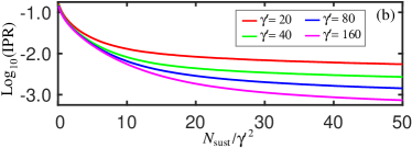
Fixed velocity erosion trajectories are calculated for irregular protoclasts with 2000 distinct realizations of disorder. A range of toughness parameter values from to are considered with the mean number of facets exceeding 4000 for the latter. Representative examples of relevant variables are shown in Fig. 22 with the sphericity complements and and the IPR shown in panel (a) and (b) while oblateness and prolateness measures are shown in panel (c) with the primordial facet survival probability plotted in panel (d). As in the case of the time dependent relative area results, and ellipticity measures are converged with respect to the parameter with minor discrepancies for the oblateness measure near its maximum likely due to Monte Carlo statistical error. Quantities such as measures of deviation from a spherical shape and the IPR do diverge on the semilogarithmic scale, but at later times with increasing suggesting convergence with respect to the latter. In a qualitative sense, in comparison to results in the case of the relative area scenario, fixed velocity variables evolve more rapidly initially with structural change slowing as sustained slices accumulate. This trend is compatible with the typical area of freshly exposed facets decreasing relative to the total area with decreasing remaining volume fraction .


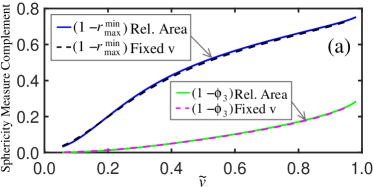
An additional merit of discussing the steady state scenario in the equilibrated regime is its relevance to non-steady state scenarios after a sufficient number of fractures have accumulated. We define an instantaneous or “effective” with where is the characteristic area exposed by a fracture event obtained by setting the exponent in the prospective slice acceptance probability to 1 and solving for the area. In the case of the fixed velocity erosion scheme, one has , which increases with decreasing remaining volume fraction. For representative variables of interest in Fig. 23, we show on the same plots equilibrated observables from steady state calculations and fixed velocity simulation results (solid or broken curves) plotted with respect to . The mean number of sites normalized with respect to , shown in panel (a), ultimately saturates at the large equilibrium value of . The IPR and complements and obtained from fixed velocity scheme simulations decrease monotonically with time in panels (b), panel (c), and panel (d) of Fig. 23, converging with steady state equilibrium results (open or filled circles). The merging of the fixed velocity simulation and equilibrium results suggests that even in non-steady state situations, stones reach a condition of quasi-equilibrium, in the sense that variables correspond closely with the steady-state counterparts calculated for after enough time has elapsed.
IV.1 General Scenario Variables from Relative Area Results


Equivalent milestones occurring at the same volume fractions remaining independent of the model (e.g. the oblateness maxima near the halfway point in the erosion of volume) is an important aspect of the deterministic time evolution of structures in spite of the stochastic nature of the collisional erosion process; in more succinct terms, graphs of relevant observables should coincide when plotted versus even for distinct models, a phenomenon which we see in Figure 24 for sample observables of interest. In panel (a), global measures of departure from a perfect spherical shape are plotted with respect to , with the solid curve gleaned from relative area calculations and the broken trace corresponding to the fixed velocity scenario. Panel (b) and (c), depicting the mean facet survival probability and the Inverse Participation Ratio also show very close agreement among the relative area and constant velocity results when plotted versus the volume fraction remaining. Finally, measures of ellipticity are displayed in panel (d) of Fig. 24, with close agreement for both the prolateness and oblateness measures. This quantitative agreement of result for distinct scenarios when plotted with respect to the remaining volume fraction has been mentioned previously Domokos1 .
The relative area scenario (i.e. ) considered in the preceding section provides an avenue for predicting the time evolution of salient observables in a broad set of cases in which the number of facets does not ultimately saturate at a finite value, but continues to rise monotonically. The universal dependence of variables on the mean volume fraction for steady state and non-steady state scenarios (e.g. the constant velocity scheme) would permit a prediction of the time dependence of variables in a wide variety of non-steady state scenarios if one knew the relationship of and for the scheme under consideration. We argue here and validate with large scale simulations involving irregular protoclasts that this mapping of onto in greater generality may be determined from steady state results as long as .
With the characteristic mean facet area being on the order of , where , the volume cleaved away by a sustained slice scales as , where is as discussed earlier a length scale related to the local radii of curvature, which we take to be on the order of , the cube root of the volume fraction. We obtain an equality with a volume dependent function , yielding for the mean volume decrement where is a series of sustained slices small in the sense that . In the large limit, one may replace and with corresponding differential quantities, and in this regime one has
| (7) |
which may be extracted numerically from data obtained in the context of the relative area scenario for (i.e. for in this work).
The characteristic function in Eq.7 in principle allows one access of for a broad range of erosion scenarios distinct from the steady state case by exploiting the fact that Solving for and integrating yields
| (8) |

Characteristic functions for cubic and irregular protoclasts are shown in Fig. 25, with solid lines representing the former and broken lines the latter. The inset graph is a magnified view of the region indicated by the pink box in the main graph for cubic protoclasts. Common to both cases is the decline from an elevated value for near unity at the beginning of the erosion process, with leveling out at a finite value for (i.e. for later times after a large portion of the original volume has eroded). This asymptotic value, indicated in the main graph and inset plots with a solid gray line, is 0.216(1) for both cube shaped and irregular protoclasts. The elevated portion of for small times is compatible with an initially accelerated loss of volume as corners and edges give way to regions of high local curvature which shed volume comparatively rapidly.
Although for the case of irregular and cube shaped counterparts appears to converge to a common asymptotic value, the characteristic function for the case of cubic protoclasts is distinct in abruptly reaching 0.216 for a finite volume fraction , where the second order phase transition to shapes lacking primordial facets occurs. The singular behavior is highlighted in the inset, which shows a magnified view of for cube shaped protoclasts with a slope discontinuity signaling the attainment of the long time value, and coinciding with the loss of primordial facets transitions indicated with the solid vertical line.
The flattening of following an initial rapid decrease provides an avenue for obtaining a closed form expression for time scales for the attainment of specific structural milestones at particular volume fractions ; given the structure of , the relationship we obtain serves as an approximation as well as a rigorous upper bound for the time needed to wear stones down to a particular volume fraction.


Curves predicted based on relative area results (solid lines) and results from direct Monte Carlo calculations (broken traces) appear in panel (a) and panel (b) of Fig. 25, respectively with log-log graphs in the inset. Broadly there is excellent agreement among the predicted and directly calculated variables.
V Salient Time Scales
Due to the universal dependence of relevant variables on volume fraction , to find time scales for a salient event such as a structural phase transition, one need only determine the volume fraction (e.g. in the context of the relative area scenario) for the case of interest and calculate the elapsed time in terms of sustained slices using Equation 8. Since decreases monotonically, ultimately converting to the asymptotic value , one has and thus time scales gleaned from Equation 8 are approximately given and bounded from above by , often amenable to exact calculation. For an power law scaling of the kinetic energy where , we obtain
| (9) |


Fig. 27 shows salient reduced time scales for a range of values of the exponent ; solid curves are obtained from Monte Carlo simulation results in the case of the relative area scenario, while broken lines are an upper bound for time scales from Equation 9. In panel (a) of Fig. 27, pertaining to cube shaped protoclasts, the two time scales shown include the structural phase transition involving the loss of primordial facets as well as the attainment of spherical shapes (corresponding to equilibration in the relative area scenario) for volume fractions and , respectively. On the other hand, in panel (b) of Fig. 27, for cohorts of irregular protoclasts, the three time scales shown correspond to , , and . In spite of the monotonic rise in for the attainment of various volume fraction milestones, panel (a) and panel (b) of Fig. 24 do not diverge for a finite value of . Moreover, the upper bound in Eq. (i.e. the same upper bound for the cases of cubic and irregular protoclasts), albeit increasing with increasing , nevertheless remains finite for finite .
VI Conclusions
In conclusion, with large scale Monte Carlo simulations, we have examined the erosion of rocks through stochastic chipping, considering polyhedral stones with as many as 3,600 facets and averaging over at least 1000 realizations of disorder. Using an energy based criterion for accepting a randomly chosen slicing plane, our calculation is unique in placing no restrictions on the number of vertices and faces sheared away with each fracture event. We have argued on theoretical grounds and verified by direct simulation that time scales for the removal of a specific amount of volume or the attainment of a particular structural milestone scale quadratically in the toughness parameter which specifies the amount of energy per area associated with a fracture; the largest time scales examined in our calculations exceed a million sustained slices per erosion sequence.
Cohorts of stochastically chipped protoclasts in the form of regular polyhedra undergo a structural phase transition in which all primordial facets are abruptly lost with concomitant singularities in other relevant observables, marking a genuine second order phase transition; in a subsequent structural transformation evident in measures of sphericity, the stones revert to spherical shapes. More broadly, however, ensemble averaged observables in the case of initially identical irregular shapes are punctuated by an elimination of facets in multiple stages instead of a single event. On the other hand, cohorts of irregular protoclasts exhibit no structural phase transitions as an aggregate, with individual eliminations of primordial surfaces being blurred by structural disorder.
We find direct measures of deviation from a spherical profile (i.e. the sphericity and ratio of minimum and maximum center of mass distances ) decrease monotonically with accumulating sustained slices. However, the oblateness measure actually rises at the initial stages of the erosion trajectory, reaching a peak when half of the original volume has been chipped away and then decreasing. This non-monotonic behavior of the oblateness is attributed to initially blade-like protoclasts which lose material more rapidly from the ends than from the edges, briefly becoming more oblate in shape before eventually being rounded into a spherical profile.
That data from distinct erosion scenarios (i.e. relative area and fixed velocity schemes) collapse onto common curves when plotted with respect to the remaining volume fraction confirms the universal dependence of observables on the latter Domokos1 . This phenomenon provides an avenue for using results in the relative area case to calculate time dependent observables for arbitrary erosion schemes, a technique we validate by reproducing results gleaned in the context of the fixed velocity scenario by direct Monte Carlo calculation. In addition, one also is afforded an efficient approach for calculating characteristic times (e.g. for specific remaining volume fractions) for a range of erosion scenarios. We have obtained closed form approximate expressions which bound these time scales from above, and which are in good quantitative agreement with the latter.
Acknowledgements.
We acknowledge helpful discussions with Michael Crescimanno. Calculations in this work have benefited from use of the Ohio Supercomputer facility (OSC) OSC .References
- (1) G Domokos, D. J. Jerolmack, A. Á.Sipos, and Á. Török, PloS One, 9, e88657 (2014).
- (2) K. L. Miller, T. Szabó, D. J. Jerolmack, and G. Domokos, Journal of Geophysical Research 10, 1002 (2014).
- (3) T. N. Szabó, A. Á Sipos, S. Shaw, D. Bertoni, A. Pozzebon, E. Grottoli, G. Sarti, P. Ciavola,G. Domokos, and D. J. Jerolmack, Sci. Adv., 4, 4946 (2018).
- (4) H. Wadell, J. Geol., 40, 443 (1932).
- (5) F. Wegner, Z. Phys. B 36, 209 (1980).
- (6) D. J. Durian, H. Bideaud, P. Duringer, A. P. Schröder, and C. M. Marques, Phys. Rev. E 75, 021301 (2007).
- (7) P. L. Krapivsky and S. Redner, Phys. Rev. E 75, 031119 (2007).
- (8) D. J. Durian, H. Bideaud, P. Duringer, A. Schröder, F. Thalmann, and C. M. Marques, Phys. Rev. Lett. 97, 028001 (2006).
- (9) F. Tonon, Journal of Mathematics and Statistics 1, 1, 8-11 (2004).
- (10) J. B. Marion and S. J. Thornton, Classical Dynamics of Particles & Systems, 3rd ed. (Harcourt, Brace, Jovanovich, Inc, Orlando, 1988).
- (11) T. N. Szabó, G. Domokos, J. B.Grotzinger, and D. J. Jerolmack, Nature Communications 6, 8366 (2015).
- (12) D. P. Landau and K. Binder, A Guide to Monte Carlo Simulations in Statistical Physics, (Cambridge, 2000).
- (13) G. Domokos, F. Kun, A. Á Sipos, and T. Szabó, Scientific Reports 5, 9147 (2015).
- (14) J. L. Howard, Sedimentology 39, 471 (1992).
- (15) Ohio Supercomputer Center. 1987. Ohio Supercomputer Center. Columbus, OH: Ohio Supercomputer Center. http://osc.edu/ark:/19495/f5s1ph73.