Time-Optimal Two- and Three-Qubit Gates for Rydberg Atoms
Abstract
We identify time-optimal laser pulses to implement the controlled-Z gate and its three-qubit generalization, the C2Z gate, for Rydberg atoms in the blockade regime. Pulses are optimized using a combination of numerical and semi-analytical quantum optimal control techniques that result in smooth Ansätze with just a few variational parameters. For the CZ gate, the time-optimal implementation corresponds to a global laser pulse that does not require single-site addressability of the atoms, simplifying experimental implementation of the gate. We employ quantum optimal control techniques to mitigate errors arising due to the finite lifetime of Rydberg states and finite blockade strengths, while several other types of errors affecting the gates are directly mitigated by the short gate duration. For the considered error sources, we achieve theoretical gate fidelities compatible with error correction using reasonable experimental parameters for CZ and C2Z gates.
1 Introduction
The improvement of fidelities for two- and multi-qubit quantum gates is a main driver of research in the field of quantum computing: High-fidelity two-qubit gates are essential for the realization of deep quantum circuits in noisy near-term digital quantum devices [1] as well as for the realization of fully-fledged fault tolerant quantum computers in the long term [2, 3, 4, 5], while high-fidelity -qubit quantum gates () may drastically reduce the gate count for quantum algorithms and enable fault tolerant quantum computation schemes adapted to specific platforms [6, 7].
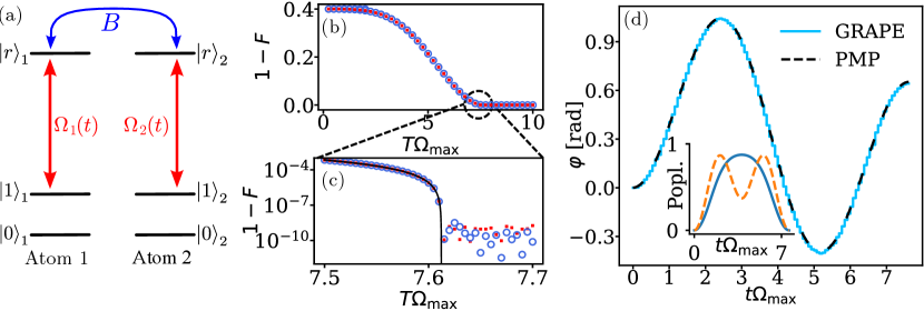
Neutral atoms are among the leading technologies for advanced analog and digital quantum simulations and have recently emerged as a highly promising platform for quantum computing [8, 9, 10, 11, 12]. Near defect-free arrays of alkali-metal and alkali-earth(-like) atoms can be routinely prepared at sub-millikelvin temperatures in optical tweezers and in optical lattices in arbitrary dimensions [13, 14, 15, 16, 17]. Fast two-qubit gates can be achieved by encoding quantum information in the internal – usually electronic ground – states of individual atoms (or collective excitations of atomic ensembles [12]) while strong interactions can be mediated by electronically highly excited Rydberg states, which can be controlled using laser fields [see Fig. 1(a)]. In the original scheme [18], the accumulation of relevant phase shifts in two-qubit quantum gates is facilitated by the so-called “Rydberg blockade” mechanism, whereby one laser-excited atom shifts the Rydberg states of neighboring atoms out of resonance due to strong Rydberg-Rydberg interactions – a process that can be readily generalized to -qubit gates, in principle [19, 20]. Two-qubit entangling gates have been implemented in several experiments [21, 22, 23, 24, 25, 26], achieving fidelities up to 99.1%. [26].
A variety of error sources limit gate fidelities in experiments, including a finite Rydberg blockade strength, decay of the Rydberg state, scattering of an intermediate state in a two photon transition, laser phase noise, variations of the laser intensity with the position of the atom in the trap and Doppler shifts of the laser frequency due to thermal motion of the atoms [22, 27, 28]. To mitigate the effects of these errors, many different improvements of the original protocol [18] have been proposed based on adiabatic passage [29, 30, 31, 32, 33, 34], dark state mechanisms [35], Rydberg Antiblockade [36, 37, 34], and many other approaches [38, 39, 40, 41, 19]. It is increasingly recognized that all these approaches can benefit from quantum optimal control methods to improve both the speed and fidelities of the various quantum gates. Quantum optimal control methods can also provide additional solutions that differ qualitatively from any of the known basic gate schemes.
Quantum optimal control methods [42] have been successfully used on a variety of platforms, including superconducting qubits [43, 44, 45, 46], trapped ions [47, 48] and neutral atoms [49, 50, 51, 52, 53, 54, 55, 56]. For neutral atoms, three properties of the laser pulses implementing a given gate are of particular interest: (i) They should be time-optimal (i.e., as short as possible) because many errors mentioned above can be mitigated by short pulse durations; (ii) They should ideally require only a global control laser addressing all atoms of the gate simultaneously – so-called global pulses –, instead of requiring single-site addressability, in order to simplify experiments; (iii) They should allow for executing three and more qubit gates natively (i.e., without decomoposing them into single- and two-qubit gates). In line with these three requirements, a remarkable result in Ref. [21] shows that a global pulse for the Controlled-Z (CZ) gate exists, which is more then 30% faster than the original, non-global proposal [18], and a global pulse exists for a Toffoli gate, albeit only with a moderate theoretically predicted fidelity of 97.6%. Naturally the question arises if it is possible to find pulses that are even faster and achieve higher fidelities, in order to make both CZ and C2Z gates fully compatible with error correction schemes.
In this work, we answer the fundamental question of identifying the fastest possible global pulse for a CZ gate and for its three-qubit generalization, the C2Z gate, satisfying the requirements (i)-(iii) above. While we assume the basic level structure of Ref. [18] (see Fig. 1(a)), our results provide original pulse schemes. Key results include: (i) For the CZ gate, we find that the time-optimal global pulse corresponds to a pulse where the laser amplitude is kept constant, while the laser phase is varied continuously and smoothly in time. The resulting pulse is about 10% faster than that of Ref. [21] – which we thus find to be already an excellent pulse. Interestingly, the found global CZ gate remains time-optimal even when considering pulses making use of single-site addressability, demonstrating that the latter is not necessary for two-qubit operations. (ii) For the C2Z gate, we find two qualitatively different time-optimal global pulses, which differ by less than 1% in speed. Interestingly, both pulses are even faster than the pulse proposed in Ref. [20], which requires single-site addressability. To our knowledge this is the first work to identify time-optimal pulses for C2Z gates. (iii) We demonstrate that the found time-optimal pulses can be adjusted to minimize errors arising from the decay of the Rydberg state or a finite blockade strength. (iv) All pulses for CZ and C2Z gates correspond to smooth time evolutions of the laser phase that can be fully described by just a few variational parameters and (v) allow for reaching theoretical fidelities compatible with most error correction schemes.
The results in this work are obtained using two complementary quantum optimal control techniques, namely Gradient Ascent Pulse Engineering (GRAPE) and Pontryagins Maximum Principle (PMP), which we combine in a novel way: The time-optimal pulses are first found using GRAPE, which requires optimization over several hundreds of parameters to describe the pulses. The pulses can then be fitted by the solution of a simple differential equation, derived using the PMP from the condition of time-optimality. In this way, the number for parameters needed to describe the pulses is reduced to only 4 and 6 for the CZ and the C2Z gate, respectively.
The paper is structured as follows: In Sec. 2 we introduce the theoretical tools used in this work. In particular, in Sec. 2.1 we introduce the level scheme and the Hamiltonian, and define the averaged fidelity as a quality measure for the implementation of a gate. We also discuss how complex conjugation or time-reversal of a laser pulse affect the implemented gate and how calculations can be simplified for global pulses. In Secs. 2.2.1 and 2.2.2 we give a brief introduction to GRAPE and the PMP, respectively. In Sec. 3 we use GRAPE to find the time-optimal global pulses that implement a CZ and a C2Z gate in the limit of an infinitely large blockade strength. In Sec. 4 we then use the PMP to give a semi-analytical description of the time-optimal pulses found in Sec. 3. In Sec. 5 we change the optimization objective and use GRAPE to identify pulses that are the most robust against decay of the Rydberg state. In Sec. 6 we discuss how the time-optimal gates from Sec. 3 can be modified to compensate for a finite blockade strength. For this, we consider two approaches: In Sec. 6.1 we assume a fixed and known blockade strength and find pulses that implement a CZ or C2Z gate exactly only at this specific blockade strength, while in Sec. 6.2 we find pulses that implement a CZ or C2Z gate exactly only at infinite blockade strength, but whose error increases as slowly as possible if the blockade strength is decreased. In Sec. 7 we calculate the fidelity for the time-optimal pulses from Sec. 3 for specific experimental parameters. Section 8 presents the conclusions.
All pulses found in this work are available at Ref. [57].
2 Theoretical Tools
In this section we introduce the theoretical tools that are used to derive optimal pulses in the subsequent sections. Section 2.1 introduces the Hamiltonian and presents the basic properties of pulses implementing a quantum gate. Section 2.2 gives a brief introduction to GRAPE, followed by an introduction to the application of the PMP method to time-optimal control.
2.1 Hamiltonians and Pulses
In Sec. 2.1.1 we first introduce the level scheme and the corresponding Hamiltonian that are used in remainder of the work. In Sec. 2.1.2 we introduce phase gates, of which the CZ gate and the C2Z gate are two examples, and show how the gate error of a pulse aiming to implement a phase gate is calculated. In Sec 2.1.3 we discuss how complex conjugation and/or time reversal of a pulse affect the implemented gate and show that in general there is not only one time-optimal pulse for a given gate, but several pulses which are related by symmetry operations. Finally, in Sec. 2.1.4 we focus on global pulses and show how some calculations simplify for them.
2.1.1 General Hamiltonian
Consider atoms treated as three-level systems: A qubit is stored in states and , which can be taken to be hyperfine states of the ground state manifold. Additionally, a Rydberg state is used to mediate the interactions between the qubits. This work focuses on the cases and to describe two- and three-qubit gates.
The level scheme for is shown in Fig. 1(a). The states and of the -th atom are coupled by a laser with time-dependent Rabi frequency . The Rabi frequency is taken to be complex, encoding both the amplitude and the phase of the laser. For this reason, no additional detuning of the laser is included, since the laser detuning and the laser phase are related through . In any experiment, the maximal achievable Rabi frequency is limited by the laser power and waist diameter. To include this into the model, a maximum Rabi frequency is introduced and only pulses with are considered for the rest of the paper.
The inter-atomic interaction term shifts the energy of the atoms and that are prepared in the Rydberg state, with called the blockade strength. This results in the Hamiltonian (with )
| (1) | ||||
The Hamiltonian (1) ignores any Rydberg-laser induced light shifts on , and . These light shifts can be cancelled by adjusting the laser frequency and by applying additional single qubit rotations around the axis after the pulse.
In previous studies, blockade strengths up to GHz have been considered [32, 38]. In Appendix A we provide a concrete example of how a blockade strength of MHz can be achieved in experiments, taking fully into account the dipole-dipole interaction between all relevant Rydberg states. The corresponding gate pulse errors for blockade strengths between are calculated in Sec. 7. We note that the coupling between the electronic and the motional degree of freedom [58] is not treated explicitly in Eq. (1). However, we expect that the gate errors arising due to this coupling are mitigated by the short gate durations of the time-optimal pulses.
For we denote by the projector onto the space spanned by all states such that atom is in state iff . For example, at we have , and (Here and in the following, a bra or a ket vector without a subscript means that this vector describes the state of all atoms, e.g. ). Since the lasers only couple to , is block-diagonal with respect to the , i.e.
| (2) |
This block-diagonality allows for solving the time evolution of a computational basis state by solving the Schrödinger equation for instead of , which reduces the dimension of the relevant Hilbert space. This will simplify the use of GRAPE and PMP methods in Secs. 3 and 4.
2.1.2 Phase Gates and Gate Error
Because any quantum gate has to map a state in the computational subspace back to and is block diagonal with respect to the , the only quantum gates that can be implemented with Eq. (1) are phase gates.
Given laser pulses of duration , we denote by the time evolution operator. The pulse is said to implement a phase gate if
| (3) |
Note that since only phase gates with can be implemented. A phase gate on qubits is, up to single qubit gates, a CZ gate if . A phase gate on qubits is, up to single qubit gates, a C2Z gate if and and all permutations of the second equation hold.
The averaged fidelity of a pulse aiming to implement a phase gate is defined by
| (4) |
where is the desired phase gate and the integral is taken over all normalized states in and with respect to the Haar measure on the unit sphere . The integral can be evaluated to [59]
| (5) | ||||
Interestingly, the fidelity can be found by propagating a single (unnormalized) state – namely – under , since by the bock-diagonality of it holds that . The so called gate error is used in the following as a quality measure for a pulse aiming to implement a phase gate. In Sec. 3, GRAPE will be used to time-optimally steer to by minimizing the gate error, which then provides a time-optimal pulse to implement the phase gate by considering the evolution of a single state only.
For the specific case of a CZ gate as a phase gate the Bell state fidelity is commonly used instead of the averaged fidelity [58, 22, 21, 38] . The Bell state fidelity measures the quality of a pulse by the fidelity between the state obtained by applying the pulse to and the desired output state . It is thus given by , which can be generalized to arbitrary phase gates as
| (6) |
Comparing Eq. (5) and Eq. (6) shows that the averaged fidelity puts more emphasis on errors leading outside of the computational subspace than the Bell state fidelity. In this work we use the averaged fidelity. We expect that the same pulses can be obtained by optimizing the Bell state fidelity instead.
2.1.3 Symmetry Operations
The time-optimal pulse implementing a phase gate is not necessarily unique, as other pulses implementing the same or a related gate can be obtained by symmetry operations. Here, three of these symmetry operations are discussed: Phase shifts, time-reversal, complex conjugation.
Given a pulse of duration implementing a phase gate for a blockade strength , several other pulses with the same duration can be constructed that implement a phase gate using the following symmetry operations
-
a)
Phase shifts: , and , for constants . To prove this statement, we denote here and in the following by the Hamiltonian given by the pulses and blockade strengths according to Eq. (1). Further, let be the time evolution operator under . Then with the basis change we have . Hence , thus also .
-
b)
Time reversal: , and . To prove that, we first show that another symmetry is given by , and . To see this, note that , so the time evolution operator under is . Hence . Together with the symmetry under phase shifts, symmetry under time reversal follows.
-
c)
Complex conjugation: , and . To prove this, we note that joint time reversal and complex conjugation is a symmetry, given by , and . To see this, note that , so the time-evolution operator under is . Hence . Together with symmetry under time reversal, symmetry under complex conjugation follows.
These three symmetry operations show that when using numerical methods to find the time-optimal pulse for a gate, several solutions are to be expected. Firstly, two time-optimal pulses can differ by an arbitrary constant phase. This degree of freedom can be eliminated by restricting the discussion to pulses where is real and positive, as we will do from now on. Even with this restriction there are in general two different time-optimal pulses for a given phase gate, related by joint complex conjugation and time reversal. In the special case of and for phase gates where all are real, which is studied in Sec. 3, there are in general even four different time-optimal pulses, because also individual time reversal or complex conjugation give pulses implementing the same gate. As will be apparent in Sec. 3, sometimes, but not always, time-optimal pulses are invariant under joint time-reversal and complex conjugation, reducing the number of distinct time-optimal pulses to two.
2.1.4 Global Pulses
This work focuses primarily on so called global pulses, where . In fact, except in Sec. 3.2, all considered pulses will be global. Global pulses can be implemented with just a single global laser addressing all atoms at the same time, no single-site addressability being needed. They are thus expected to be easier to realize experimentally. When working with global pulses it will be further assumed (except briefly in Sec. 6) that all are equal to the same blockade strength .
The theoretical treatment using global pulses is simplified compared to the general case in two different ways: Firstly, now it holds that if and have the same number of 1s. As a consequence, only phase gates with can be implemented. For the whole gate is then determined by the evolution of under , and the fidelity is given by
| (7) | ||||
with . Similarly, for the whole gate is determined by the evolution of under , with
| (8) | ||||
The second simplification due to global pulses is a simplification of Hamiltonians if contains two or more 1s. For we have
| (9) | ||||
with . The rank of thus reduces from generally 4 to 3 in the global case. For we make the analogous simplification
| (10) |
To simplify , we note that the only states that can be accessed from with a global pulse are , and . It is thus sufficient to consider just the projection of onto the symmetric subspace , given by
| (11) |
This reduces the rank of from generally 8 to 4 in the global case.
This discussion concludes the presentation of the basic properties of pulses implementing phase gates, and of global pulses in particular. After a brief introduction to GRAPE and the PMP in the following subsection, the theoretical discussion from this section will be used in Secs. 3 and 4 to identify the time-optimal pulses for the CZ gate and the C2Z gate.
2.2 Quantum Optimal Control Methods
In this section we give a brief introduction to GRAPE and the PMP, the two quantum optimal control methods used in this work.
2.2.1 GRAPE Algorithm
Gradient Ascent Pulse Engineering (GRAPE) is a quantum optimal control technique based on gradient descent. It was originally developed to design pulse sequences for NMR spectroscopy, and has been used successfully to speed up quantum gates and to increase the fidelity of pulses in the presence of imperfections [60, 61, 62, 63]. In the context of neutral atoms GRAPE has been used to design arbitrary gates in the hyperfine levels of CS [54, 55, 56].
Given an initial state , a pulse duration and a Hamiltonian depending on controls , GRAPE can be used to find the optimal controls , minimizing , for an arbitrary objective function . For this, a piecewise constant Ansatz for is made, i.e. if and , with the number of pieces. Typically, several hundreds of pieces are used. Minimizing becomes an optimization problem over . GRAPE provides a fast way to calculate all derivatives , which then allows for the efficient use of a gradient descent algorithm to find a local minimum of the cost function. In our implementation, we use the Broyden–Fletcher–Goldfarb–Shanno algorithm [64, 65] as the gradient descent method.
2.2.2 Pontryagin’s Maximum Principle for Time-Optimal Control
Pontryagin’s Maximum principle (PMP) [66, 67, 68] is an optimal control technique that has been used successfully to find time-optimal [69, 70, 71, 61] or robust [72] quantum gates, and to optimize variational quantum algorithms [73]. The PMP is an analytic principle that gives a set of necessary conditions that optimal pulses have to satisfy, thereby allowing to reduce the infinite dimensional control landscape to a low-dimensional space [72]. In contrast to GRAPE, which usually uses several hundreds of variational parameters, the PMP can therefore describe optimal pulses with just a handful of parameters. On the downside, the PMP does not provide a universal algorithm to find the parameters leading to the optimal pulse. In Sec. 4 we will combine GRAPE and the PMP to describe the pulses found by GRAPE using the PMP with just 4 parameters for the CZ and 6 parameters for the C2Z gate.
In this section we give a formulation of the PMP and apply it to the problem of time-optimal pulses on Rydberg atoms. We start by formulating the PMP for the specific case of time-optimal control problems [67]: Suppose one wants to steer a real vector from an initial point to a final point using the differential equation , where describe the available controls (i.e., the Rabi frequencies of the lasers in our case). Later, will correspond to the quantum state and will be given by Schrödinger’s equation. We call a triplet a controlled trajectory if , and . The PMP gives necessary conditions on the controlled trajectory that minimizes , where is an arbitrary cost function.
By focusing on time-optimal control problems, we can fix . In this case, the PMP then states that for a given time-optimal controlled trajectory there exist so-called costates with values in such that at each time the following equations are satisfied
| (12) |
and
| (13) |
where denotes the scalar product. Further, if the are restricted to a submanifold of , the can be restricted to the tangent space of at [74]. If the supremum in Eq. (13) is only achieved by a single value of the controls, the PMP allows to reduce the search for the time-optimal trajectory to the search over the initial costates , which determine the full trajectory via Eqs. (12) and (13).
In this work, we directly apply the PMP to the Schrödinger equation . This is done by decomposing the state and the Hamiltonian into real and imaginary parts [70, 71], which results in two real costates and . By combining the two real costates with a complex one as , Eq. (12) becomes the Schrödinger equation for the costates, while Eq. (13) reads [71]
| (14) | ||||
The key point is that, as long as the supremum is achieved at a unique value of the controls, the initial states and costates completely determine the optimal trajectory.
Applied to time-optimal phase gates the PMP states that there are costates evolving under the Schrödinger equation such that
| (15) | ||||
where the sum can be either over all , or for global pulses with or only over or , respectively.
In Sec. 4 we will use the PMP to reproduce the results found by GRAPE by extracting the initial costates from the pulses found by GRAPE. This allows us to describe the time-optimal pulses just through the initial costates, which correspond to 4 parameters for the CZ gate and 6 parameters for the C2Z gate.
3 Time-Optimal Gates at Infinite Blockade Strength ()
In this section we use GRAPE to find the time-optimal pulses in the limit . In this limit states with more than one atom in the Rydberg state cannot be populated, because the lasers coupling them to states with one atom in the Rydberg state are infinitely far detuned. We start by considering the CZ gate in Sec. 3.1 and find that the time-optimal global pulse is approximately 10% faster than the pulse of Ref. [21]. In Sec. 3.2 we then show that allowing for individual adressability for the atoms brings no speedup for the CZ gate, which is one of the main results of the work. Finally, in Sec. 3.3 we find the time-optimal global pulse for the three-qubit C2Z gate, and a second, slightly slower global pulse that also implements a C2Z gate. All found pulses are smooth functions of the parameters.
3.1 Global CZ Gate
In this section we apply GRAPE to find the time-optimal global pulse that implements a CZ gate in the setup of Fig. 1(a) with . We say that a pulse implements a CZ gate if it implements a phase gate with , and for some single qubit phase . By additional single qubit gates compensating the phase of gained by and , a CZ gate with can be achieved.
As discussed in Sec. 2.1, the action of a global pulse is completely described by the evolution of under the Hamiltonian
| (16) |
where the matrix representation is in the basis. Since the state can never be populated, it is omitted from the description.
The time-optimal pulse must have maximal amplitude for all , because if at some time it had sub-maximal amplitude, the pulse could be sped up by simply increasing and shortening the pulse accordingly. Since the Hamiltonian is proportional to , this operation only speeds up the gate, but does not change the trajectory of . Therefore, the Ansatz is made. To find the time-optimal we start by fixing a pulse duration and use GRAPE to minimize the gate error , as given in Eq. (7), over the laser phase and the single qubit rotation angle . GRAPE is initialized with a random guess for and .
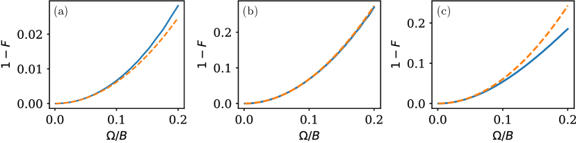
The minimal gate error computed by GRAPE for for dimensionless pulse durations between 0 and is shown by blue circles in Fig. 1b). At the gate error is 0.4, corresponding to the identity gate with . As is increased, the minimal gate error drops and reaches 0 around . We find that for GRAPE can converge to two different values of , one of them being the sub-optimal gate error 0.4 – corresponding to the identity. In the interesting range , however, a unique value of is found for all runs of the algorithm. To precisely determine the duration of the time-optimal pulse we plot the gate errors in the range in log scale in Fig. 1(c). The gate errors drop until they are of order of , which corresponds to the chosen convergence criterion of the optimization. We fit the gate errors with
| (17) |
and extract the time-optimal pulse duration for the CZ gate. The form of the fitting function is motivated by the observation that should vanish in the first order of , otherwise negative gate errors would be possible for . The resulting time-optimal pulse is about 10% faster then the pulse in Ref. [21] with , showing a relevant speedup of the gate. Our results also show that the duration of the pulse in Ref. [21] is already quite close to the achievable minimum.
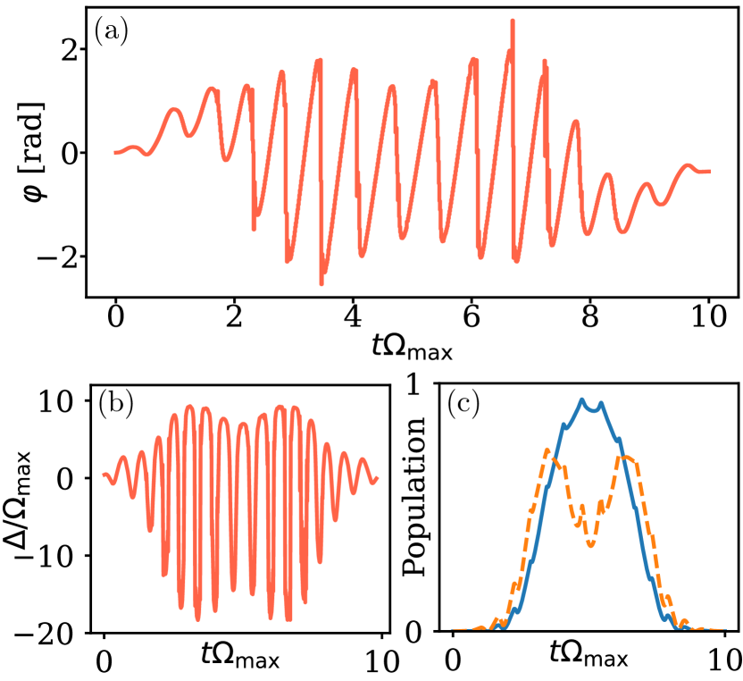
The laser phase that leads to the time-optimal pulse as obtained by the GRAPE algorithm is shown as a solid blue line in Fig. 1(d) as a function of the dimensionless time . The shape of is the piecewise constant approximation of a smooth curve, which resembles, but is not identical to, a sine wave with a linear offset: It first increases to (at ), then decreases to (at ), and finally increases again to . We show below in Sec. 4 using the PMP that the piecewise constant curve found by GRAPE is in fact the discrete approximation of a “true” time-optimal pulse, which is smooth [dashed black curve in Fig. 1(d)]. Note that our pulse is significantly simpler, and thus easier to implement, than the pulses found in Refs. [50, 51], which also apply optimal control techniques. Our pulse is also more than three times faster than the pulse found in Ref. [24] by optimizing the amplitude of while assuming a fixed laser detuning. We attribute this to our approach of including the laser phase in the optimization, and to our use of the simplest possible model of the system, which allows to identify the fundamentally time-optimal pulse regardless of experimental imperfections.
As discussed in Sec. 2.1.3 above, a pulse implementing a CZ gate can also be obtained by complex conjugation and/or time-reversal of the pulse shown in Fig. 1(d). No sign flip of is necessary during this symmetry operations, because a pulse implementing a certain phase gate at implements the same phase gate at . When applying complex conjugation or time reversal, the single qubit rotation angle needs to be changed to . For the time-optimal global pulse for the CZ gate, complex conjugation and time reversal coincide, so there are only two time-optimal global pulses: The pulse in Fig. 1(d) and the complex conjugated pulse.
The occupation probabilities of (or ) – when starting in (or ) – and – when starting in – as a function of are shown in the Inset of Fig. 1(d) as a blue solid curve and an orange dashed curve, respectively. The figure shows that the populations of (and ) and have a maximum and a local minimum at , respectively. This is due to the fact that since the coupling between and is times stronger than the coupling between and the population of changes with a faster rate than that of .
3.2 CZ Gate with single-site addressability
A natural question is whether the pulse from the previous section can be sped up by allowing single-site addressability of the atoms. Here we find that this is not the case.
In order to identify the time-optimal non-global pulse, we proceed just like for global pulses above, except that now two independent lasers described by complex and are considered: We thus proceed by minimizing the gate error [see Eq. (5)] over both phase and amplitude of and (not shown). Now the evolution of could in principle be different from that of and the state could evolve to arbitrary states in the , subspace. However, as shown by the red squares in Fig. 1b)c), the minimal gate error is not reduced when allowing for non-global instead of global pulses. Hence also when allowing for single-site addressability, the time-optimal pulse satisfies , where describes the time-optimal global pulse found above. Single-site addressability thus brings no speed advantage for the implementation of a CZ gate. This is one of the main results of the paper.
3.3 Global C2Z Gate
For the global three-qubit C2Z gate we follow a similar protocol as for the 2-qubit CZ gate. The goal is to implement a phase gate with , and . Up to single qubit rotations of around the z-axis, this implements the gate . We use GRAPE to minimize the gate error with the fidelity given in Eq. (8), the initial state , and the Hamiltonian , given as a matrix by
| (18) |
in the basis.
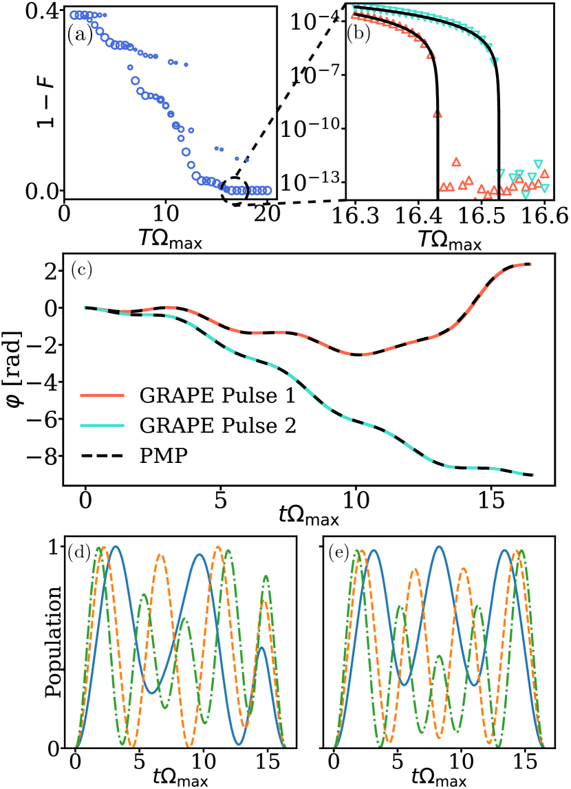
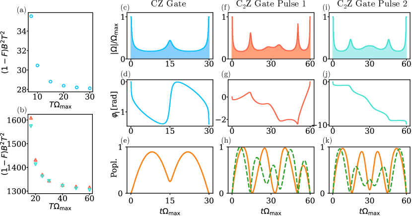
Figure 2(a) shows the gate error as a function of the dimensionless pulse duration in the range , as obtained for the C2Z gate using GRAPE. In the figure, the size of the blue dots is proportional to the number of times that each gate error was obtained in the given set of GRAPE runs. The figure shows that the lowest gate errors form a smooth curve made of larger dots – corresponding to more frequent convergences of the algorithm – with several plateaus. Minimal gate errors with values are reached around . In order to precisely determine the optimal , Fig. 2(b) shows a zoom-in of the results of panel (a) in the interesting range , in log-scale. The figure shows the existence of two distinct curves with very similar : The first curve, called “Pulse 1” from now on, has a , while the second one, called “Pulse 2”, has a . Both pulses are faster then the original non-global implementation with [20]. The two pulses result from rather different , which are shown in Fig. 2(c): The laser phase for Pulse 1 oscillates from 0 to -2.6 and then back to about 2.3, while the phase of Pulse 2 is monotonically decreasing from 0 to approximately -9.0. Again equivalent pulses can be obtain by time-reversal and complex conjugation of Pulse 1 and Pulse 2. For Pulse 1 this leads to four different pulses, for Pulse 2 only to two different pulses, since time-reversal and complex conjugation coincide. Figures 2(d) and (e) show the population during Pulse 1 and Pulse 2, respectively, of , (blue solid line), (orange dashed line), and (green dash-dotted line). The three types of populations are found to oscillate approximately with the frequencies , and that are expected if the laser phase is kept constant. Populations in Pulse 2 are further found to be symmetric with respect to time-reversal.
This concludes Sec. 3, in which GRAPE was applied to find the time-optimal global pulses for the CZ and the C2Z gate. For both gates the time-optimal pulse is faster then the traditional non-global pulse, for the CZ gate additionally % faster than the pulse in Ref. [21]. All pulses are, up to the discretization introduced by GRAPE, simple and smooth pulses. For the CZ gate we additionally found that allowing for individual addressability of the atoms brings no speedup of the gate.
4 Semi-Analytical Description of the Pulses using the PMP
| CZ Pulse | C2Z Pulse 1 | C2Z Pulse 2 | |
| 0.11212523i | 0.23064809i | 0.18360502i | |
| -0.70546052 | 0.06339133 | 0.11567664 | |
| -0.21533291i | +0.42859775i | +0.46913157i | |
| -0.06056999i | -0.55488096i | -0.54588492i | |
| 0.51526141 | 0.18981665 | 0.14734489 | |
| -0.41739917i | -0.03941303i | -0.04548695i | |
| 0.29436027i | 0.30789524i | ||
| -0.19206657 | -0.18760792 | ||
| -0.53858404i | -0.53014859i | ||
| 7.6114828 | 16.426439 | 16.532211 | |
The pulses found by GRAPE are piecewise constant functions obtained using 99 and 399 parameters for the CZ and the C2Z gate, respectively. In the following, the PMP is used to demonstrate that the latter functions are in fact discrete approximations of smooth pulses that are solutions of ordinary differential equations with just 4 and 6 parameters for the CZ and the C2Z gates, respectively.
In order to apply the PMP to the time-optimal global CZ and C2Z gates at , the maximization condition (15) has to be formulated for and as a function of the laser phase . The Hamiltonians are, in the appropriate basis,
| (19) |
with the number of 1s in and and the Pauli X- and Y-matrices, respectively. The maximization condition (15) is
| (20) |
with summed over for the CZ gate and for the C2Z gate. Note that contrary to many other applications of the PMP to quantum optimal control [70, 71, 69, 73, 61], in our case the Hamiltonian depends on the control in a non-linear way. Therefore, the optimal control is not given by a so-called “bang-bang” pulse, but by a continuous function .
The maximization in Eq. (20) then leads to
| (21) |
with
| (22) | ||||
| (23) |
Given the initial costates , the whole pulse can be determined from Eq. (21) and the Schrödinger equation for states and costates, as long as the quantity does not vanish during the pulse. The time-optimal pulse is now found by minimizing the gate error calculated from the final states over the initial costates and the pulse duration . This reduces the control landscape from an infinite dimensional space to a 4-dimensional space for the CZ gate ( and are both two-dimensional vectors) and a 6-dimensional space for the C2Z gate. Since the are constrained on the manifold, the costates can be restricted to the tangent space of this manifold, so they can be chosen such that for all .
In Ref. [72], optimal pulses for the robust control of a two-level system haven been successfully obtained by the use of a gradient descent algorithm in the reduced control landscape. In our case however, such an optimization proved to be unsuccessful without a good initial guess for the , because small variations in the initial costates can lead to large variations in the final states. Therefore, we introduce the following new procedure to obtain a good initial guess of the based on the pulses found by GRAPE: Denote by the time evolution operator under , so that . Equation (20) then implies that for all
| (24) | ||||
with
| (25) |
GRAPE gives the states, controls and time-evolution operators at discrete times . Letting we obtain
| (26) |
Now the real and imaginary parts of all are combined into a single real matrix , and the real and imaginary parts of all into a single real vector , such that Eq. (26) just becomes . To find approximate, nonzero solutions to this linear equation is decomposed as . An approximate solution to , and thus a good initial guess for , is given either by or by , where is the singular vector with the smallest, approximately zero, singular value .
Using this approximate solution as a starting point of the minimization of the gate error over the initial costates and the pulse duration using the Powell method [65] the optimized values in Table 1 are obtained. Using Eq. (20) together with the Schrödinger equation for the states and costates then allows one to reconstruct the pulses found by GRAPE directly from the initial costates. We find that these pulses reconstructed by the PMP are in excellent agreement with the pulses found by GRAPE, as can be seen from Fig. 1(d) and Fig. 2(c). These results demonstrate that the pulses found by GRAPE are simply discrete approximations of smooth time-optimal pulses, which can be obtained by just a few variational parameters. This procedure allows for immediate reproducibility of the time-optimal pulses using the few parameters in Table 1 and Eq. (20) together with the Schrödinger equation for the states and costates only.
5 Minimizing the Decay of the Rydberg State
In the following, we focus on obtaining global pulses for the CZ and C2Z gates that achieve the highest fidelity in the presence of a finite lifetime of the Rydberg state. For this a non-Hermitian term is added to the Hamiltonian of each atom, where is the decay rate of the chosen Rydberg state . This term describes the loss of population from the subspace of the Hilbert space and thus slightly overestimates the gate error, since it neglects the fact that spontaneous decay of the Rydberg state may repopulate the or state [35]. As shown in Appendix B, the gate error of a pulse that leads to an exact CZ or C2Z in the decay-free case is now given by for . Here, is the average time that the atoms spend in the Rydberg state, as given by
| (27) |
where and is the projector onto the subspace with one atom in the Rydberg state. Our goal is to minimize over all pulses that implement a CZ or C2Z gate with fidelity 1 in the decay-free case. For this, is chosen and minimized using GRAPE. Because the resulting pulses still have a fidelity in the decay-free case. Because the resulting pulses minimize over all pulses with fidelity 1 in the decay free case.
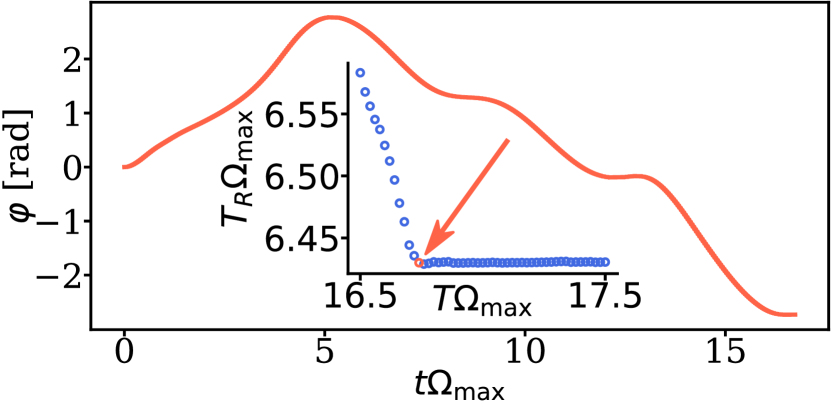
To use GRAPE we fix , but we stress that the resulting pulse minimizes for any and thus minimizes the gate error as long as . For the CZ gate we then find that the time-optimal pulse is essentially indistinguishable from the pulse with the lowest : takes the values and for the former and the latter cases, respectively, where the latter is evaluated for a comparatively long pulse duration . On the contrary, for the C2Z gate the minimal is improved with respect to both Pulses 1 and 2 found above (which have and , respectively). This is shown in the Inset of Fig. 3, which displays for the pulses leading to the lowest gate errors in the range : is found to sharply decrease to a value at and then to stay constant for larger . We have checked that this behavior persists for comparatively long times of at least – twice as long as the time-optimal pulse. The pulse improves by about 7% and 14% over the of the time-optimal Pulses 1 and 2, respectively, clearly demonstrating that in general the time-optimal pulse is not identical to the pulse with the smallest average time in the Rydberg state for the three-qubit C2Z gate. Consistently, Fig. 3 shows that the phase of the pulse that minimizes at is qualitatively different from that of both time-optimal Pulses 1 and 2 found above (see Fig. 2(c)).
These results demonstrate that GRAPE can also be used to find the pulse minimizing the time spent in the Rydberg state, instead of the total pulse duration. While for the CZ gate the time-optimal pulse coincides with the pulse minimizing , for the C2Z gate a slight reduction of compared to the time-optimal pulse can be achieved.
6 Gates at Finite Blockade Strength
The assumption can never be achieved in a real experiment, so it is a natural question to ask how pulses can operate at finite . There are at least two approaches to this problem: In the first approach, treated in Sec. 6.1, is assumed to take a fixed value, and global pulses are optimized to achieve fidelity only at this specific value of . However, in many experiments is not known with high precision, because it depends on the distance between the atoms, which cam fluctuate due to thermal motion. For this reason the second approach, treated in Sec. 6.2, aims to find global pulses that achieve fidelity only at , but are affected as weakly as possible as is decreased.
6.1 Fixed Blockade Strength
In the first approach, treated in this section, a finite is fixed and GRAPE is used to find the time-optimal pulses. We begin by discussing CZ gate, where the time-optimal pulses at a finite are close to the time-optimal pulses at . Then we find that for the C2Z gate there is in fact a pulse at finite that is much faster then the time-optimal pulse at . This pulse significantly populates states with two atoms in the Rydberg state and thus accesses parts of the Hilbert space that are inaccessible in the limit. Finally we show that also for the C2Z gate pulses with fidelity 1 at finite can be found that are close to the time-optimal pulses. As a way of example, we take for the rest of this subsection.
6.1.1 Time-Optimal CZ Gate
Just like in Sec. 3.1 for , we now use GRAPE at a finite interaction strength . The only modification is that now the state has to be included, so the pulse is completely describe by the evolution of under the Hamiltonian
| (28) |
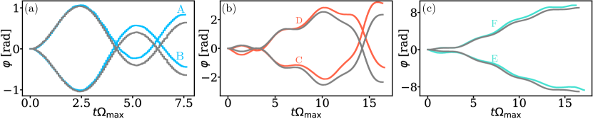
in the basis. We find two different pulses with similar pulse duration: The first pulse, “Pulse A”, with qualitatively resembles the pulse from Fig. 1(d), while the second, slightly longer, “Pulse B” with qualitatively resembles the complex conjugated version of the pulse from Fig. 1(d). Pulse A and Pulse B are shown together with the two time-optimal pulses in the case in Fig. 4a. Pulse A is slightly faster, pulse B slightly slower then the time-optimal pulse for . Both pulses achieve a gate error below , showing that even for a finite it is possible to implement an exact CZ gate.
6.1.2 Speeding up the C2Z gate
For the C2Z gate the effects of a finite blockade strength depend on the positioning of the atoms relative to each other. Here we assume that the blockade strength is the same for any pair of atoms. In the case of an isotropic blockade strength this can be achieved by placing the atoms on the vertices of an equilateral triangle, the so-called triangular arrangement [75]. Another possibility is the so-called linear arrangement, in which the three atoms are arranged in a one-dimensional chain, so the distance between the two outer atoms is twice the distance between an outer and the inner atom. We discuss this linear arrangement briefly at the end of this section and in Appendix C.
When applying GRAPE to find the time-optimal pulse for a C2Z gate in the triangular arrangement at a finite , pulses with a duration significantly below the duration of the time-optimal pulse in the case are found. As an example, at there exists a pulse with duration and gate error , which is shown in Fig. 5(a). The phase of this pulse varies rapidly with , such that the detuning is of the order of [Fig. 5(b)]. This suggests that this pulse operates in the so-called Rydberg antiblockade regime [76] where states with two atoms in the Rydberg state can become significantly populated. This is confirmed by the populations of and , that are shown as a function of in Fig.5(c) as blue solid line and orange dashed line, respectively. The pulse therefore speeds up the C2Z gate by using states with two atoms in the Rydberg state, which is not possible in the case. Naturally one would expect such a pulse to be very sensitive to variations of , and indeed when decreasing by just 10% the gate error increases drastically to . At a finite it is therefore possible to significantly speed up the C2Z gate at the cost of a high sensitivity to variations in the blockade strength. Since the blockade strength depends strongly on the distance of the atoms, this pulse is only feasible if the distance between the atoms is known with high precision.
6.1.3 Pulses for the C2Z Gate resembling the pulses
In order to find pulses for the C2Z gate that more are robust against variations of the blockade strength, we now determine pulses at finite that are close to the time-optimal pulses. For this, we start by the approximation that the effects of a finite can be completely captured by an ac-Stark shift of the states with one atom in the Rydberg state. This approximation is justified in in Sec. 6.2 and in more detail in Appendix D through a time dependent Schrieffer-Wolff transformation. Since in this approximation the Hamiltonians are close to the Hamiltonians in the case, we also expect the time-optimal pulses to be close to Pulse 1 and Pulse 2. With this approximation, and are given by
| (29) | ||||
and
| (30) |
GRAPE is used to find the time-optimal pulses under this approximation. These pulses are then used as initial guesses for GRAPE with the exact Hamiltonian. Through this procedure, pulses with fidelity at finite resembling the pulses are found. Pulses C and D, close to Pulse 1 and its complex conjugated version, respectively, are shown Fig. 5(b). Their durations are and . Pulses E and F, close to Pulse 2 and its complex conjugated version, respectively, are shown in Fig. 5(c), with durations and . All pulses have a gate error at They are also significantly less susceptible to variations of than the faster pulse found above, i.e. reducing by 10% never increases the gate error to more then . This is an improvement by three orders of magnitude compared to the faster pulse found above.
For the linear instead of the triangular arrangement it is shown in Appendix C that, under the approximation that the effects of a finite can be completely captured by an ac-Stark shift and in the limit, there exist no pulses with fidelity close to the pulses. Qualitatively, this is caused by different pairs of atoms being affected differently by the finite , but in the same way by the global laser.
In summary, the results of this section show that for both the CZ and the C2Z gate in the triangular arrangement the time-optimal pulses at can be modified to compensate for a finite value of . For the C2Z gate it is even possible to significantly decrease the gate duration in the finite case by a pulse which significantly populates states with two atoms in the Rydberg state. This comes at the downside of a much larger sensitivity to variations in . Note that for the CZ gate a similar speedup of the gate is not possible. All results were obtained at . We expect that the picture remains qualitatively the same as long as .
6.2 Variable Blockade Strength
Instead of designing a pulse to work at a specific blockade strength , in this section only pulses that have fidelity at are considered. Within the set of these pulses, the pulses that are affected the least by a finite are identified. To this end, it is shown in Appendix D using a time dependent Schrieffer-Wolff transformation [77] that to first order in all effects of the finiteness of can be described by an ac-Stark shift of the energy of the states with one atom in the Rydberg state. For the CZ gate this means modifying to
| (31) |
where we split . We also expand the state as .
As shown in Appendix E, a pulse with fidelity in the case has at finite a gate error of
| (32) | ||||
To lowest order, the gate error thus increases quadratically with . Our goal is now to use GRAPE to minimize , as given by the right hand side of Eq. (32). Note that this minimizes the gate error simultaneously for all values of for which contributions of order and higher can be neglected.
To apply GRAPE, and are treated as independent states satisfying
| (33) |
Eq. (33) now replaces the Schrödinger Equation for in the formulation of GRAPE.
To minimize over all states with fidelity in the case, the objective function for GRAPE is taken as
| (34) |
Here, is a large constant ensuring that only pulses with fidelity close to 1 in the case can minimize . We take and verify that indeed the gate errors at are always below .
Given a pulse with duration that implements a CZ gate at , the gate error at finite can be reduced by an arbitrary factor , for , by simply stretching the pulse to duration and taking . To see this, note that is decreased by , while the pulse duration is increased by . Hence is decreased by , and according to Eq. (32) by . To compare different pulses beyond a stretch, the dimensionless quantity is taken as a quality measure for pulses from now on.
Using Eq. (32), the time-optimal pulse for the CZ gate is found to have . To improve upon this, GRAPE is now used to minimize over both the amplitude and the phase of the laser pulse at a fixed , using the time-optimal pulse stretched to duration as initial guess. The minimal values of for values of between 7.61 and 30 are shown in Fig. 6(a). decreases as the pulse duration increases, but asymptotically approaches a non-zero value around as , which is an improvement of over 20% compared to the time-optimal pulse. The amplitude and the phase of at are shown in Figs. 6(c) and (d) respectively. The amplitude starts maximal, then drops to about 25% after a quarter of the pulse duration. Towards the middle of the pulse the amplitude increases again to around 50%, then it decreases again to 25% at three quarters of the pulse duration and finally increases to the maximal amplitude at the end of the pulse. This behavior can be understood by considering the population of , the only state affected by the ac-Stark shift due to the finite . The population of , shown in Fig. 6(e), starts at 0 and increases to 0.9 at . It then decreases to 0.25 at and increases again to 0.9 at , before dropping to 0 at the end of the pulse. Notably, the laser amplitude is inversely correlated to the population . Through this, whenever the population of is large, the laser amplitude, and thus also the ac-Stark shift of , is reduced.
For the C2Z gate in the triangular arrangement the ac-Stark shift due to the finite leads to and as given in Eqs. (29) and (30). A formula for the gate error depending on and analogous to Eq. (32) is derived in Appendix E [Eq. (55)]. Again is used as a quality measure for different pulses, the time-optimal Pulse 1 has , the slightly slower Pulse 2 has . GRAPE is applied with either Pulse 1 or Pulse 2 as initial guess to minimize for between 16.6 and 60, shown in Fig. 6(b) with red upward pointing triangles for Pulse 1 as initial guess and turquoise downward pointing triangles for Pulse 2 as initial guess. For both cases decreases when is increased and asymptotically approaches for both pulses, an improvement of 30% over the time-optimal Pulse 1 and of 20% over Pulse 2 . The amplitude and phase for the pulse minimizing at when initializing GRAPE with pulse 1 are shown in Figs. 6(f) and (g) respectively, the amplitude and phase when initializing GRAPE with Pulse 2 in Figs. 6(i) and (j) respectively. The laser amplitude is again inversely correlated to the populations and , shown in Fig. 6(h) and (k) as orange solid line and green dashed line respectively, and displays several peaks at times where the population of these states is small.
The results in this section show that both for the CZ and for the C2Z gate the time-optimal pulses can be improved to decrease the effect of a finite blockade strength at the cost of a longer pulse duration. The improvement of the gate error goes beyond simply stretching the pulses and is based on a modulation of the laser amplitude to reduce the ac-Stark shift when the states affected by it are populated most.
7 Gate Errors for a Specific Setup
Finally, in this section we calculate the gate errors of the time-optimal pulses found above at a specific blockade strength and decay rate of the Rydberg state. The same setup as in [32] is chosen, with the qubits encoded in the clock states of Caesium and the Rydberg state . At 300K the Rydberg state has a lifetime of . Adding the error contributions from the decay of the Rydberg state and due to a finite blockade strength and neglecting all other error sources, the gate error is given by
| (35) |
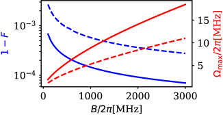
The gate error can now be minimized by varying while keeping and fixed and thus balancing the trade-off between the error due to decay of the Rydberg state and due to a finite blockade strength. The minimal gate errors and the optimal values of for the CZ gate and Pulse 1 for the C2Z gate are shown in Fig. 7. At the maximal considered blockade strength the minimal gate errors are for the CZ and for Pulse 1 for the C2Z gate in the triangular arrangement. For the blockade strength MHz, which is shown to be achievable in Appendix A, the gate errors are for the CZ gate and for the C2Z gate. The required Rabi frequencies take realistic values of the order of . For Pulse 2 for the C2Z gate (not shown in Fig. 7) the gate error is always slightly above the gate error for Pulse 1, at most by 8%. Additionally, the optimal Rabi frequency is also always slightly above that for Pulse 1, at most by 7%.
In summary, these results show that moderate blockade strengths around MHz and moderate Rabi frequencies around MHz are sufficient to achieve gate errors of order of for both the CZ and the C2Z gate. Even lower gate errors can be achieved by higher blockade strengths and larger Rabi frequencies. For the calculations above, the time-optimal pulses from Sec. 3, which were optimized at , were used. For the gates from Sec. 6.1, which were optimized at a finite , the gate error arises solely due to the decay of the Rydberg state and is inversely proportional to . Only the errors due to a finite blockade strength and decay of the Rydberg state were considered in the calculations above.
8 Conclusion
In this work the time-optimal global pules for the CZ and the C2Z gate in the blockade regime were identified. The pulse durations of for the CZ gate and for the C2Z gate improve even upon the traditional, non-global pulses [18, 20] and upon the recently discovered global pulse for the CZ gate with [21]. Due to the shortest possible pulse duration, most types of errors which become more detrimental for longer gate durations, like the decay of the Rydberg state or Doppler shifts of the laser frequency, are mitigated. Since the pulses are global, they can be realized by a single laser addressing all atoms simultaneously. No single-site addressability is needed, thus significantly simplifying the experimental requirements. Interestingly, for the CZ gate single-site addressability even brings no speedup over the time-optimal global pulse, showing that single-site addressability, which requires a more complex experimetal setup, is not always advantageous.
The results were obtained using the quantum optimal control techniques GRAPE and PMP, which we combined in a novel way. GRAPE allowed to find the time-optimal pulses in the first place, using several hundreds of variational parameters. The PMP then allowed to reduce the variational parameters to just 4 for the CZ and 6 for the C2Z gate, thus showing that the pulses found by GRAPE are indeed the piecewise constant approximation of a simple smooth pulse given by the solution of an ordinary differential equation. The description by the PMP allows for immediate reproducibility of the time-optimal pulses just from the parameters in Table 1 and without using GRAPE again.
GRAPE was also used to optimize the robustness of pulses for a CZ and C2Z gate against the decay of the Rydberg state and against errors arising due to a finite blockade strength. To mitigate the effects of the decay of the Rydberg state, the average time spent in the Rydberg state was minimized. Interestingly, for the CZ gate the time-optimal pulse coincides with the pulse minimizing the time in the Rydberg state, while for the C2Z gate a small improvement is possible. Two approaches were taken to mitigate the effects of a finite blockade strength: In the first approach, pulses were optimized at a fixed, finite value of and it was shown that the time-optimal pulses can be modified to compensate for the finiteness of . In the second approach, pulses were identified that implement a CZ or C2Z gate exactly at infinite blockade strength while minimizing the second derivative of the gate error with respect to the inverse blockade strength. The first approach works best if the blockade strength is known exactly, while the second approach gives a pulse that works well for all large blockade strengths.
Finally, the gate errors were calculated for a plausible experimental setup using the state of Caesium as the Rydberg state. Gate errors as low as for the CZ gate and for the C2Z gate can be achieved at GHz and Rabi frequencies of the order of MHz. At the much weaker blockade strength of MHz still gate errors of for the CZ gate and for the C2Z gate can be achieved.
The results show that quantum optimal control techniques, especially GRAPE and the PMP, are versatile tools to design gates on Rydberg atoms. In this work, only gates that make use of a single Rydberg state per atom and that operate in the blockade regime were considered. While most gates in current experiments are of this kind, it is known that more robust gates can be achieved when using several Rydberg states per atom [35, 78], and ultrafast gates can be achieved by operating outside of the Rydberg blockade regime [79]. We expect that quantum optimal control techniques can also be used to improve these gates.
Data Availability
All pulse shapes found in this work are available at Ref. [57].
Acknowledgments
We are grateful to Shannon Whitlock and Frank Wilhelm-Mauch for stimulating discussions. This research has received funding from the European Union’s Horizon 2020 research and innovation programme under the Marie Skłodowska-Curie grant agreement number 955479. G. P. acknowledges support from the Institut Universitaire de France (IUF) and the University of Strasbourg Institute of Advanced Studies (USIAS).
Appendix A Estimation of the Effective Blockade Strength
In this appendix we calculate which effective blockade strength can be achieved when using Caesium atoms, and , and aligning the atoms perpendicular to quantization axis. This is the same setup as assumed in [32, 38]. The interaction between two atoms at a distance is given by the dipole-dipole potential
| (36) |
where denotes the 3d position operator of atom and is the unit vector along the line interconnecting the atoms. The system of two atoms is then described by the Hamiltonian
| (37) |
where denote single atom Rydberg states and () is the binding energy of the Rydberg state ().
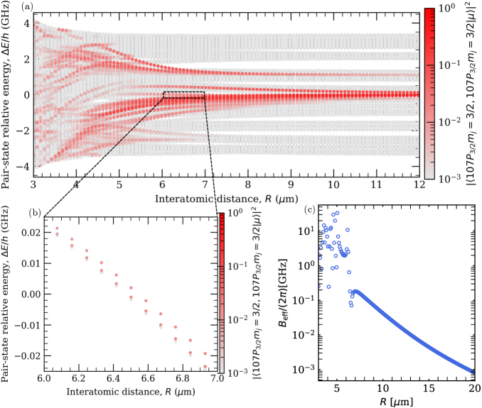
Using the Alkali.ne Rydberg Calculator (ARC) package [80], can be easily calculated and diagonalized. To find the effective blockade strength (defined below), we diagonalized , taking into account all Rydberg states with principle quantum number and with orbital quantum number . The eigenvalues for between 3m and 12m are shown in Fig. 8(a), with the color indicating the squared overlap between the corresponding eigenstate and . It can be seen that, contrary to the simple model in Fig. 1(a), there are several eigenstates with a significant overlap with . Since the effects of a finite blockade strength are well approximated through an ac-Stark shift of the state (see Appendix D), we define the effective blockade strength as the blockade strength which correctly reproduces the ac-Stark shift of coming from the coupling to all . This effective blockade strength has been introduced under the name frequency shift factor before [81]. can be calculated as
| (38) |
where is the energy of (relative to the energy of in the absence of the dipole-dipole interaction), describes the laser coupling the state to the Rydberg states and is the Rabi frequency of this laser for the coupling between and .
is shown as a function of in Fig. 8(c). When decreasing from infinity, increases monotonically until m, where it suddenly drops. This drop can be explained by two eigenstates of becoming resonant () around m, which is shown in Fig. 8(b). These two eigenstates consist primarily of states, with a squared overlap summed over all magnetic quantum numbers of 0.56. The squared overlap with is 0.02 for both states.
For m the effective blockade strength changes rapidly and non-monotonously with . We therefore take the maximal achievable blockade strength to be the maximal for m, which is given by MHz at m.
Appendix B Gate Error due to Decay
In this appendix, we show that a pulse of duration which implements a phase gate with fidelity in the absence of decay has a gate error of when a decay of the Rydberg state with decay rate with is included. For this, denote by the Hamiltonian from Eq. (1) and by the nonhermitian term added to the Hamiltonian to describe decay. Further, denote by and the time evolution operator from to under and , respectively. We use the abbreviations and . Then to first order in we have
| (39) |
Now we use that and that to obtain
| (40) |
where and . Note that for the case, where there is at most one atom in the Rydberg state, is the projector onto the states with exactly one atom in the Rydberg state.
Appendix C The C2Z Gate in the Linear Arrangement
In this appendix we discuss the C2Z gate in the linear arrangement, in which three atoms are aligned in a row. There, the outer two atoms, labeled atoms 1 and 3 from now on, are separated by a larger distance than an outer and the middle atom (labeled 2). Thus, there are two different blockade strengths: and . In the van der Waals regime where the blockade strength is proportional to , with the interatomic distance, we have , but the following arguments will hold for all with .
Let be a global pulse of duration that implements a C2Z gate at , for example Pulse 1 or Pulse 2 from Sec. 3.3. We will show that if there is no small change such that implements a C2Z gate at blockade strengths .
Denote by the Hamiltonian under as defined in Eq. (2) at , and by the perturbation of the Hamiltonian due the change of the laser pulse and due to the finite Blockade strength. In the limit we can treat the finite blockade strength through an ac-Stark shift (see Appendix D) and obtain
| (42) |
and
| (43) |
with and . Now we denote by the time evolution operator from to under , set = and define analogously with . Then
| (44) |
For the C2Z gate we require . We obtain with that
| (45) |
and
| (46) |
with
| (47) |
and
| (48) |
where again .
Because and behave identically up to relabeling the qubits, we obtain and . Since and , it follows from Eqs. (45) and (46) that . Hence the pulse does not implement a C2Z gate. Qualitatively, this is because the and are effected differently by a finite blockade strength, but identically by a change in .
Appendix D Approximation of a Finite Blockade Strength through an AC-Stark Shift
Let be a global pulse with duration that implements a CZ or C2Z with fidelity 1 at . In this appendix we use a time dependent Schrieffer-Wolff transformation (TDSWT) [77] to show that the the final state can be obtained to first order in just by including an ac-Stark shift to the Hamiltonian, modifying to
| (49) |
and and as in Eqs. (29) and (30). We only show this explicitly for the CZ gate, the statement for the C2Z gate follows completely analogously.
The goal of a TDSWT is to make a time dependent basis transformation , where is an anti-hermitian matrix, such that evolves under a Hamiltonian that does not couple the state to the or state anymore. For this, we split with
| (50) |
We expand and where and are of order . There is no term, because in the limit , already does not couple to or . From this limit we can also infer and . According to the TDSWT, and can be found by (see Eqs. (6) and (7) in Ref. [77]):
| (51) |
| (52) |
Solving Eqs. (51) and (52) gives
| (53) |
We conclude that to first order in we can treat the effects of a finite just through an ac-Stark shift, as long as we consider instead of . However, we are only interested in at and , and at both times is, to 0th order in , proportional to . Because we thus have at these two times . To describe the effects of a finite up to first order in , it is therefore sufficient to just consider the ac-Stark shift of and use instead of . We remark that terms of order are either proportional to or to . To neglect these terms, is therefore not sufficient, additionally has to hold. Analogously, to be able to neglect terms of higher orders, has to hold for all . If oscillates with a frequency of the order of , as for example for the pulse in Sec. 6.1.2, this does not hold and the effect of a finite can not described solely by an ac-Stark shift.
Appendix E Gate Error of a CZ and C2Z Gate to Second Order in
In this appendix we derive perturbative expressions for the gate error at finite for pulses that implement a CZ or C2Z with fidelity in the case. For this, we expand and show that for the CZ gate it holds that
| (54) |
while for the C2Z gate in the triangular arrangement it holds that
| (55) | ||||
To derive both formulas, we use two ingredients: Firstly any quantity depending on satisfies
| (56) |
Secondly, for any normalized vector depending on and with it holds that
| (57) |
so that
| (58) |
and
| (59) |
For the fidelity of a CZ gate we obtain from Eq. (7) with and that
| (60) |
Now we apply Eq. (56). Because the pulse has fidelity 1 in the case we have and , so that
| (61) | ||||
By inserting Eqs. (58) and (59) into Eq. (61) we obtain Eq. (54).
For the C2Z gate we obtain from Eq. (8) with and that
| (62) | ||||
We apply Eq.(56) and use that , and to obtain
| (63) | ||||
By inserting Eqs. (58) and (59) into Eq. (63) we obtain Eq. (55).
We numerically confirm Eqs. (54) and (55) as well as the fact that to first order in it is sufficient to account for the finiteness of through an ac-Stark shift (see Appendix D). For this, we consider the time-optimal pulse for the CZ gate and Pulse 1 and Pulse 2 for the C2Z gate (see Sec. 3) and calculate the gate error once using the exact Hamiltonian and once from Eqs. (54) and (55). In the latter case, the are found through Eq. (33). The exact and the approximate gate error are shown in Fig. 9 as blue solid line and orange dotted line, respectively. For all three considered pulses the exact and the approximate gate error are in excellent agreement for large .
References
- Preskill [2018] John Preskill. Quantum Computing in the NISQ era and beyond. Quantum, 2:79, 2018. doi: 10.22331/q-2018-08-06-79.
- Svore et al. [2007] K.M. Svore, D.P. DiVincenzo, and B.M. Terhal. Noise threshold for a fault-tolerant two-dimensional lattice architecture. QIC, 7:297–318, 2007. doi: 10.26421/QIC7.4-2.
- Fowler et al. [2012] Austin G. Fowler, Matteo Mariantoni, John M. Martinis, and Andrew N. Cleland. Surface codes: Towards practical large-scale quantum computation. Phys. Rev. A, 86:032324, 2012. doi: 10.1103/PhysRevA.86.032324.
- Spedalieri and Roychowdhury [2009] Federico M. Spedalieri and Vwani P. Roychowdhury. Latency in local, two-dimensional, fault-tolerant quantum computing. QIC, 9:666–682, 2009. doi: 10.26421/QIC9.7-8-9.
- Lai et al. [2014] Ching-Yi Lai, Gerardo Paz, Martin Suchara, and Todd A. Brun. Performance and error analysis of Knill’s postselection scheme in a two-dimensional architecture. QIC, 14:807–822, 2014. doi: 10.26421/QIC14.9-10-7.
- Baker et al. [2021] Jonathan M. Baker, Andrew Litteken, Casey Duckering, Henry Hoffmann, Hannes Bernien, and Frederic T. Chong. Exploiting Long-Distance Interactions and Tolerating Atom Loss in Neutral Atom Quantum Architectures. In 2021 ACM/IEEE 48th Annual International Symposium on Computer Architecture (ISCA), pages 818–831, Valencia, Spain, 2021. IEEE. ISBN 978-1-66543-333-4. doi: 10.1109/ISCA52012.2021.00069.
- Cong et al. [2021] Iris Cong, Sheng-Tao Wang, Harry Levine, Alexander Keesling, and Mikhail D. Lukin. Hardware-Efficient, Fault-Tolerant Quantum Computation with Rydberg Atoms. arXiv:2105.13501, 2021. doi: 10.48550/arXiv.2105.13501.
- Bloch et al. [2008] Immanuel Bloch, Jean Dalibard, and Wilhelm Zwerger. Many-body physics with ultracold gases. Rev. Mod. Phys., 80:885–964, 2008. doi: 10.1103/RevModPhys.80.885.
- Saffman et al. [2010] M. Saffman, T. G. Walker, and K. Mølmer. Quantum information with Rydberg atoms. Rev. Mod. Phys., 82:2313–2363, 2010. doi: 10.1103/RevModPhys.82.2313.
- Browaeys and Lahaye [2020] Antoine Browaeys and Thierry Lahaye. Many-body physics with individually controlled Rydberg atoms. Nat. Phys., 16:132–142, 2020. doi: 10.1038/s41567-019-0733-z.
- Henriet et al. [2020] Loïc Henriet, Lucas Beguin, Adrien Signoles, Thierry Lahaye, Antoine Browaeys, Georges-Olivier Reymond, and Christophe Jurczak. Quantum computing with neutral atoms. Quantum, 4:327, 2020. doi: 10.22331/q-2020-09-21-327.
- Morgado and Whitlock [2021] M. Morgado and S. Whitlock. Quantum simulation and computing with Rydberg-interacting qubits. AVS Quantum Sci., 3:023501, 2021. doi: 10.1116/5.0036562.
- Endres et al. [2016] Manuel Endres, Hannes Bernien, Alexander Keesling, Harry Levine, Eric R. Anschuetz, Alexandre Krajenbrink, Crystal Senko, Vladan Vuletic, Markus Greiner, and Mikhail D. Lukin. Atom-by-atom assembly of defect-free one-dimensional cold atom arrays. Science, 354:1024–1027, 2016. doi: 10.1126/science.aah3752.
- Barredo et al. [2016] Daniel Barredo, Sylvain de Léséleuc, Vincent Lienhard, Thierry Lahaye, and Antoine Browaeys. An atom-by-atom assembler of defect-free arbitrary two-dimensional atomic arrays. Science, 354:1021–1023, 2016. doi: 10.1126/science.aah3778.
- Ohl de Mello et al. [2019] Daniel Ohl de Mello, Dominik Schäffner, Jan Werkmann, Tilman Preuschoff, Lars Kohfahl, Malte Schlosser, and Gerhard Birkl. Defect-Free Assembly of 2D Clusters of More Than 100 Single-Atom Quantum Systems. Phys. Rev. Lett., 122:203601, 2019. doi: 10.1103/PhysRevLett.122.203601.
- Barredo et al. [2018] Daniel Barredo, Vincent Lienhard, Sylvain de Léséleuc, Thierry Lahaye, and Antoine Browaeys. Synthetic three-dimensional atomic structures assembled atom by atom. Nature, 561:79–82, 2018. doi: 10.1038/s41586-018-0450-2.
- Schlosser et al. [2019] Malte Schlosser, Sascha Tichelmann, Dominik Schäffner, Daniel Ohl de Mello, Moritz Hambach, and Gerhard Birkl. Large-scale multilayer architecture of single-atom arrays with individual addressability. arXiv:1902.05424, 2019. doi: 10.48550/arXiv.1902.05424.
- Jaksch et al. [2000] D. Jaksch, J. I. Cirac, P. Zoller, S. L. Rolston, R. Côté, and M. D. Lukin. Fast Quantum Gates for Neutral Atoms. Phys. Rev. Lett., 85:2208–2211, 2000. doi: 10.1103/PhysRevLett.85.2208.
- Müller et al. [2009] M. Müller, I. Lesanovsky, H. Weimer, H. P. Büchler, and P. Zoller. Mesoscopic Rydberg Gate Based on Electromagnetically Induced Transparency. Phys. Rev. Lett., 102:170502, 2009. doi: 10.1103/PhysRevLett.102.170502.
- Isenhower et al. [2011] L. Isenhower, M. Saffman, and K. Mølmer. Multibit C k NOT quantum gates via Rydberg blockade. Quantum Inf Process, 10:755–770, 2011. doi: 10.1007/s11128-011-0292-4.
- Levine et al. [2019] Harry Levine, Alexander Keesling, Giulia Semeghini, Ahmed Omran, Tout T. Wang, Sepehr Ebadi, Hannes Bernien, Markus Greiner, Vladan Vuletić, Hannes Pichler, and Mikhail D. Lukin. Parallel Implementation of High-Fidelity Multiqubit Gates with Neutral Atoms. Phys. Rev. Lett., 123:170503, 2019. doi: 10.1103/PhysRevLett.123.170503.
- Graham et al. [2019] T. M. Graham, M. Kwon, B. Grinkemeyer, Z. Marra, X. Jiang, M. T. Lichtman, Y. Sun, M. Ebert, and M. Saffman. Rydberg-Mediated Entanglement in a Two-Dimensional Neutral Atom Qubit Array. Phys. Rev. Lett., 123:230501, 2019. doi: 10.1103/PhysRevLett.123.230501.
- Picken et al. [2018] C J Picken, R Legaie, K McDonnell, and J D Pritchard. Entanglement of neutral-atom qubits with long ground-Rydberg coherence times. Quantum Sci. Technol., 4:015011, 2018. doi: 10.1088/2058-9565/aaf019.
- Fu et al. [2022] Zhuo Fu, Peng Xu, Yuan Sun, Yang-Yang Liu, Xiao-Dong He, Xiao Li, Min Liu, Run-Bing Li, Jin Wang, Liang Liu, and Ming-Sheng Zhan. High-fidelity entanglement of neutral atoms via a Rydberg-mediated single-modulated-pulse controlled-phase gate. Phys. Rev. A, 105:042430, 2022. doi: 10.1103/PhysRevA.105.042430.
- Martin et al. [2021] Michael J. Martin, Yuan-Yu Jau, Jongmin Lee, Anupam Mitra, Ivan H. Deutsch, and Grant W. Biedermann. A Mølmer-Sørensen Gate with Rydberg-Dressed Atoms. arXiv:2111.14677, 2021. doi: 10.48550/arXiv.2111.14677.
- Madjarov et al. [2020] Ivaylo S. Madjarov, Jacob P. Covey, Adam L. Shaw, Joonhee Choi, Anant Kale, Alexandre Cooper, Hannes Pichler, Vladimir Schkolnik, Jason R. Williams, and Manuel Endres. High-Fidelity Entanglement and Detection of Alkaline-Earth Rydberg Atoms. Nat. Phys., 16:857–861, 2020. doi: 10.1038/s41567-020-0903-z.
- de Léséleuc et al. [2018] Sylvain de Léséleuc, Daniel Barredo, Vincent Lienhard, Antoine Browaeys, and Thierry Lahaye. Analysis of imperfections in the coherent optical excitation of single atoms to Rydberg states. Phys. Rev. A, 97:053803, 2018. doi: 10.1103/PhysRevA.97.053803.
- Zhang et al. [2012] X. L. Zhang, A. T. Gill, L. Isenhower, T. G. Walker, and M. Saffman. Fidelity of a Rydberg-blockade quantum gate from simulated quantum process tomography. Phys. Rev. A, 85:042310, 2012. doi: 10.1103/PhysRevA.85.042310.
- Rao and Mølmer [2014] D. D. Bhaktavatsala Rao and Klaus Mølmer. Robust Rydberg-interaction gates with adiabatic passage. Phys. Rev. A, 89:030301, 2014. doi: 10.1103/PhysRevA.89.030301.
- Beterov et al. [2016] I. I. Beterov, M. Saffman, E. A. Yakshina, D. B. Tretyakov, V. M. Entin, S. Bergamini, E. A. Kuznetsova, and I. I. Ryabtsev. Two-qubit gates using adiabatic passage of the Stark-tuned Förster resonances in Rydberg atoms. Phys. Rev. A, 94:062307, 2016. doi: 10.1103/PhysRevA.94.062307.
- Mitra et al. [2020] Anupam Mitra, Michael J. Martin, Grant W. Biedermann, Alberto M. Marino, Pablo M. Poggi, and Ivan H. Deutsch. Robust Mølmer-Sørensen gate for neutral atoms using rapid adiabatic Rydberg dressing. Phys. Rev. A, 101:030301, 2020. doi: 10.1103/PhysRevA.101.030301.
- Saffman et al. [2020] M. Saffman, I. I. Beterov, A. Dalal, E. J. Paez, and B. C. Sanders. Symmetric Rydberg controlled-Z gates with adiabatic pulses. Phys. Rev. A, 101:062309, 2020. doi: 10.1103/PhysRevA.101.062309.
- Beterov et al. [2020] I. I. Beterov, D. B. Tretyakov, V. M. Entin, E. A. Yakshina, I. I. Ryabtsev, M. Saffman, and S. Bergamini. Application of adiabatic passage in Rydberg atomic ensembles for quantum information processing. J. Phys. B: At. Mol. Opt. Phys., 53:182001, 2020. doi: 10.1088/1361-6455/ab8719.
- He et al. [2021] Yucheng He, Jing-Xin Liu, F.-Q. Guo, Lei-Lei Yan, Ronghui Luo, Erjun Liang, Shi-Lei Su, and M. Feng. Multiple-qubit Rydberg quantum logic gate via dressed-states scheme. arXiv:2010.14704, 2021. doi: 10.48550/arXiv.2010.14704.
- Petrosyan et al. [2017] David Petrosyan, Felix Motzoi, Mark Saffman, and Klaus Mølmer. High-fidelity Rydberg quantum gate via a two-atom dark state. Phys. Rev. A, 96:042306, 2017. doi: 10.1103/PhysRevA.96.042306.
- Wu et al. [2021a] Jin-Lei Wu, Yan Wang, Jin-Xuan Han, Shi-Lei Su, Yan Xia, Yongyuan Jiang, and Jie Song. Unselective ground-state blockade of Rydberg atoms for implementing quantum gates. arXiv:2107.09975, 2021a. doi: 10.1007/s11467-021-1104-7.
- Wu et al. [2021b] Jin-Lei Wu, Yan Wang, Jin-Xuan Han, Shi-Lei Su, Yan Xia, Yongyuan Jiang, and Jie Song. Resilient quantum gates on periodically driven Rydberg atoms. Phys. Rev. A, 103:012601, 2021b. doi: 10.1103/PhysRevA.103.012601.
- Theis et al. [2016] L. S. Theis, F. Motzoi, F. K. Wilhelm, and M. Saffman. High-fidelity Rydberg-blockade entangling gate using shaped, analytic pulses. Phys. Rev. A, 94:032306, 2016. doi: 10.1103/PhysRevA.94.032306.
- Liu et al. [2022] Shuai Liu, Jun-Hui Shen, Ri-Hua Zheng, Yi-Hao Kang, Zhi-Cheng Shi, Jie Song, and Yan Xia. Optimized nonadiabatic holonomic quantum computation based on Förster resonance in Rydberg atoms. Front. Phys., 17:21502, 2022. doi: 10.1007/s11467-021-1108-3.
- Shen et al. [2019] Cai-Peng Shen, Jin-Lei Wu, Shi-Lei Su, and Erjun Liang. Construction of robust Rydberg controlled-phase gates. Opt. Lett., 44:2036, 2019. doi: 10.1364/OL.44.002036.
- Guo et al. [2020] Chen-Yue Guo, L.-L. Yan, Shou Zhang, Shi-Lei Su, and Weibin Li. Optimized geometric quantum computation with a mesoscopic ensemble of Rydberg atoms. Phys. Rev. A, 102:042607, 2020. doi: 10.1103/PhysRevA.102.042607.
- Glaser et al. [2015] Steffen J. Glaser, Ugo Boscain, Tommaso Calarco, Christiane P. Koch, Walter Köckenberger, Ronnie Kosloff, Ilya Kuprov, Burkhard Luy, Sophie Schirmer, Thomas Schulte-Herbrüggen, Dominique Sugny, and Frank K. Wilhelm. Training Schrödinger’s cat: Quantum optimal control: Strategic report on current status, visions and goals for research in Europe. Eur. Phys. J. D, 69:279, 2015. doi: 10.1140/epjd/e2015-60464-1.
- Egger and Wilhelm [2014] D. J. Egger and F. K. Wilhelm. Optimized controlled Z gates for two superconducting qubits coupled through a resonator. Supercond. Sci. Technol., 27:014001, 2014. doi: 10.1088/0953-2048/27/1/014001.
- Kelly et al. [2014] J. Kelly, R. Barends, B. Campbell, Y. Chen, Z. Chen, B. Chiaro, A. Dunsworth, A. G. Fowler, I.-C. Hoi, E. Jeffrey, A. Megrant, J. Mutus, C. Neill, P. J. J. O’Malley, C. Quintana, P. Roushan, D. Sank, A. Vainsencher, J. Wenner, T. C. White, A. N. Cleland, and John M. Martinis. Optimal Quantum Control Using Randomized Benchmarking. Phys. Rev. Lett., 112:240504, 2014. doi: 10.1103/PhysRevLett.112.240504.
- Huang and Goan [2014] Shang-Yu Huang and Hsi-Sheng Goan. Optimal control for fast and high-fidelity quantum gates in coupled superconducting flux qubits. Phys. Rev. A, 90:012318, 2014. doi: 10.1103/PhysRevA.90.012318.
- Werninghaus et al. [2021] M. Werninghaus, D. J. Egger, F. Roy, S. Machnes, F. K. Wilhelm, and S. Filipp. Leakage reduction in fast superconducting qubit gates via optimal control. npj Quantum Inf, 7:14, 2021. doi: 10.1038/s41534-020-00346-2.
- Nebendahl et al. [2009] V. Nebendahl, H. Haffner, and C. F. Roos. Optimal control of entangling operations for trapped ion quantum computing. Phys. Rev. A, 79:012312, 2009. doi: 10.1103/PhysRevA.79.012312.
- Choi et al. [2014] T. Choi, S. Debnath, T. A. Manning, C. Figgatt, Z.-X. Gong, L.-M. Duan, and C. Monroe. Optimal Quantum Control of Multimode Couplings between Trapped Ion Qubits for Scalable Entanglement. Phys. Rev. Lett., 112:190502, 2014. doi: 10.1103/PhysRevLett.112.190502.
- Goerz et al. [2011] Michael H Goerz, Tommaso Calarco, and Christiane P Koch. The quantum speed limit of optimal controlled phasegates for trapped neutral atoms. J. Phys. B: At. Mol. Opt. Phys., 44:154011, 2011. doi: 10.1088/0953-4075/44/15/154011.
- Müller et al. [2011] M. M. Müller, D. M. Reich, M. Murphy, H. Yuan, J. Vala, K. B. Whaley, T. Calarco, and C. P. Koch. Optimizing entangling quantum gates for physical systems. Phys. Rev. A, 84:042315, 2011. doi: 10.1103/PhysRevA.84.042315.
- Goerz et al. [2014] Michael H. Goerz, Eli J. Halperin, Jon M. Aytac, Christiane P. Koch, and K. Birgitta Whaley. Robustness of high-fidelity Rydberg gates with single-site addressability. Phys. Rev. A, 90:032329, 2014. doi: 10.1103/PhysRevA.90.032329.
- Omran et al. [2019] A. Omran, H. Levine, A. Keesling, G. Semeghini, T. T. Wang, S. Ebadi, H. Bernien, A. S. Zibrov, H. Pichler, S. Choi, J. Cui, M. Rossignolo, P. Rembold, S. Montangero, T. Calarco, M. Endres, M. Greiner, V. Vuletić, and M. D. Lukin. Generation and manipulation of Schrödinger cat states in Rydberg atom arrays. Science, 365:570–574, 2019. doi: 10.1126/science.aax9743.
- Cui et al. [2017] Jian Cui, Rick van Bijnen, Thomas Pohl, Simone Montangero, and Tommaso Calarco. Optimal control of Rydberg lattice gases. Quantum Sci. Technol., 2:035006, 2017. doi: 10.1088/2058-9565/aa7daf.
- Smith et al. [2013] A. Smith, B. E. Anderson, H. Sosa-Martinez, C. A. Riofrío, Ivan H. Deutsch, and Poul S. Jessen. Quantum Control in the Cs 6 S 1 / 2 Ground Manifold Using Radio-Frequency and Microwave Magnetic Fields. Phys. Rev. Lett., 111:170502, 2013. doi: 10.1103/PhysRevLett.111.170502.
- Anderson et al. [2015] B. E. Anderson, H. Sosa-Martinez, C. A. Riofrío, Ivan H. Deutsch, and Poul S. Jessen. Accurate and Robust Unitary Transformations of a High-Dimensional Quantum System. Phys. Rev. Lett., 114:240401, 2015. doi: 10.1103/PhysRevLett.114.240401.
- Lysne et al. [2020] Nathan K. Lysne, Kevin W. Kuper, Pablo M. Poggi, Ivan H. Deutsch, and Poul S. Jessen. Small, Highly Accurate Quantum Processor for Intermediate-Depth Quantum Simulations. Phys. Rev. Lett., 124:230501, 2020. doi: 10.1103/PhysRevLett.124.230501.
- Jandura and Pupillo [2022] Sven Jandura and Guido Pupillo. Figshare data repository, 2022. URL https://doi.org/10.6084/m9.figshare.19658427.
- Robicheaux et al. [2021] F. Robicheaux, T. M. Graham, and M. Saffman. Photon-recoil and laser-focusing limits to Rydberg gate fidelity. Phys. Rev. A, 103:022424, 2021. doi: 10.1103/PhysRevA.103.022424.
- Pedersen et al. [2007] Line Hjortshøj Pedersen, Niels Martin Møller, and Klaus Mølmer. Fidelity of quantum operations. Physics Letters A, 367:47–51, 2007. doi: 10.1016/j.physleta.2007.02.069.
- Khaneja et al. [2005] Navin Khaneja, Timo Reiss, Cindie Kehlet, Thomas Schulte-Herbrüggen, and Steffen J. Glaser. Optimal control of coupled spin dynamics: Design of NMR pulse sequences by gradient ascent algorithms. Journal of Magnetic Resonance, 172:296–305, 2005. doi: 10.1016/j.jmr.2004.11.004.
- Garon et al. [2013] A. Garon, S. J. Glaser, and D. Sugny. Time-optimal control of SU(2) quantum operations. Phys. Rev. A, 88:043422, 2013. doi: 10.1103/PhysRevA.88.043422.
- Riaz et al. [2019] Bilal Riaz, Cong Shuang, and Shahid Qamar. Optimal control methods for quantum gate preparation: A comparative study. Quantum Inf Process, 18:100, 2019. doi: 10.1007/s11128-019-2190-0.
- Wilhelm et al. [2020] Frank K. Wilhelm, Susanna Kirchhoff, Shai Machnes, Nicolas Wittler, and Dominique Sugny. An introduction into optimal control for quantum technologies. arXiv:2003.10132, 2020. doi: 10.48550/arXiv.2003.10132.
- Nocedal and Wright [2006] Jorge Nocedal and Stephen J. Wright. Numerical Optimization. Springer Series in Operation Research and Financial Engineering. Springer, New York, NY, 2. ed edition, 2006. ISBN 978-1-4939-3711-0 978-0-387-30303-1.
- Jones et al. [2001] Eric Jones, Travis Oliphant, Pearu Peterson, and others. SciPy: Open source scientific tools for Python, 2001.
- Pontryagin and Neustadt [1986] L. S. Pontryagin and Lucien W. Neustadt. The Mathematical Theory of Optimal Processes. Classics of Soviet Mathematics. Gordon and Breach Science Publishers, New York, english ed edition, 1986. ISBN 978-2-88124-077-5.
- Lee and Markus [1986] E. B. Lee and L. Markus. Foundations of Optimal Control Theory. R.E. Krieger Pub. Co, Malabar, Fla, 1986. ISBN 978-0-89874-807-9.
- Boscain et al. [2021] U. Boscain, M. Sigalotti, and D. Sugny. Introduction to the Pontryagin Maximum Principle for Quantum Optimal Control. PRX Quantum, 2:030203, 2021. doi: 10.1103/PRXQuantum.2.030203.
- Bao et al. [2018] Seraph Bao, Silken Kleer, Ruoyu Wang, and Armin Rahmani. Optimal control of superconducting gmon qubits using Pontryagin’s minimum principle: Preparing a maximally entangled state with singular bang-bang protocols. Phys. Rev. A, 97:062343, 2018. doi: 10.1103/PhysRevA.97.062343.
- Lin et al. [2019] Chungwei Lin, Yebin Wang, Grigory Kolesov, and Uroš Kalabić. Application of Pontryagin’s minimum principle to Grover’s quantum search problem. Phys. Rev. A, 100:022327, 2019. doi: 10.1103/PhysRevA.100.022327.
- Lin et al. [2020] Chungwei Lin, Dries Sels, and Yebin Wang. Time-optimal control of a dissipative qubit. Phys. Rev. A, 101:022320, 2020. doi: 10.1103/PhysRevA.101.022320.
- Van Damme et al. [2017] L. Van Damme, Q. Ansel, S. J. Glaser, and D. Sugny. Robust optimal control of two-level quantum systems. Phys. Rev. A, 95:063403, 2017. doi: 10.1103/PhysRevA.95.063403.
- Yang et al. [2017] Zhi-Cheng Yang, Armin Rahmani, Alireza Shabani, Hartmut Neven, and Claudio Chamon. Optimizing Variational Quantum Algorithms Using Pontryagin’s Minimum Principle. Phys. Rev. X, 7:021027, 2017. doi: 10.1103/PhysRevX.7.021027.
- Chang [2011] Dong Eui Chang. A simple proof of the Pontryagin maximum principle on manifolds. Automatica, 47:630–633, 2011. doi: 10.1016/j.automatica.2011.01.037.
- Barredo et al. [2014] D. Barredo, S. Ravets, H. Labuhn, L. Béguin, A. Vernier, F. Nogrette, T. Lahaye, and A. Browaeys. Demonstration of a Strong Rydberg Blockade in Three-Atom Systems with Anisotropic Interactions. Phys. Rev. Lett., 112:183002, 2014. doi: 10.1103/PhysRevLett.112.183002.
- Ates et al. [2007] C. Ates, T. Pohl, T. Pattard, and J. M. Rost. Antiblockade in Rydberg Excitation of an Ultracold Lattice Gas. Phys. Rev. Lett., 98:023002, 2007. doi: 10.1103/PhysRevLett.98.023002.
- Theis and Wilhelm [2017] L. S. Theis and F. K. Wilhelm. Nonadiabatic corrections to fast dispersive multiqubit gates involving Z control. Phys. Rev. A, 95:022314, 2017. doi: 10.1103/PhysRevA.95.022314.
- Khazali and Mølmer [2020] Mohammadsadegh Khazali and Klaus Mølmer. Fast Multiqubit Gates by Adiabatic Evolution in Interacting Excited-State Manifolds of Rydberg Atoms and Superconducting Circuits. Phys. Rev. X, 10:021054, 2020. doi: 10.1103/PhysRevX.10.021054.
- Chew et al. [2021] Yeelai Chew, Takafumi Tomita, Tirumalasetty Panduranga Mahesh, Seiji Sugawa, Sylvain de Léséleuc, and Kenji Ohmori. Ultrafast energy exchange between two single Rydberg atoms on the nanosecond timescale. arXiv:2111.12314, 2021. doi: 10.48550/arXiv.2111.12314.
- Šibalić et al. [2017] N. Šibalić, J.D. Pritchard, C.S. Adams, and K.J. Weatherill. ARC: An open-source library for calculating properties of alkali Rydberg atoms. Computer Physics Communications, 220:319–331, 2017. doi: 10.1016/j.cpc.2017.06.015.
- Walker and Saffman [2008] Thad G. Walker and M. Saffman. Consequences of Zeeman degeneracy for the van der Waals blockade between Rydberg atoms. Phys. Rev. A, 77:032723, 2008. doi: 10.1103/PhysRevA.77.032723.