Time-Optimal Control Studies for Additional Food provided Prey-Predator Systems involving Holling Type-III and Holling Type-IV Functional Responses

D Bhanu Prakash First Author. Email: [email protected] D K K Vamsi Corresponding author. Email: [email protected]

Abstract

In recent years, time-optimal control studies on additional food provided prey-predator systems have gained significant attention from researchers in the field of mathematical biology. In this study, we initially consider an additional food provided prey-predator model exhibiting Holling type-III functional response and the intra-specific competition among predators. We prove the existence and uniqueness of global positive solutions for the proposed model. We do the time optimal control studies with respect quality and quantity of additional food as control variables by transforming the independent variable in the control system. Making use of the Pontraygin maximum principle, we characterize the optimal quality of additional food and optimal quantity of additional food. We show that the findings of these time-optimal control studies on additional food provided prey-predator systems involving Holling type III functional response have the potential to be applied to a variety of problems in pest management. In the later half of this study, we consider an additional food provided prey-predator model exhibiting Holling type-IV functional response and study the above aspects for this system.

keywords: Time-optimal control; Pontraygin Maximum Principle; Holling type-III response; Holling type-IV response; Pest management;

MSC 2020 codes: 37A50; 60H10; 60J65; 60J70;

1 Introduction

Prey-predator models are mathematical representations used to study the intricate dynamics between two interacting species: the prey and its predator. These models aim to understand how changes in the population sizes of both species influence each other over time. By examining the fluctuations and stability of both populations, these models contribute to our understanding of ecological balance, the impact of external factors on species coexistence, and the potential consequences of perturbations in natural communities. Prey-predator models play a critical role in guiding conservation efforts, studying invasive species’ effects, and comprehending the intricate web of life in ecosystems worldwide.

One of the fundamental components in prey-predator models is the functional response which describes how the predator’s consumption rate changes in response to variations in prey density [1]. The very first few proposed functional responses are the Holling functional responses, proposed by Canadian ecologist C.S. Holling in the 1950s [2]. The Holling type-III and Holling type-IV functional responses are widely observed in real life situations. The Holling type-III functional response exhibits a slow increase in the predator’s consumption rate at low prey densities, followed by a rapid rise as prey density reaches a certain threshold. Whereas, the Holling type-IV functional response exhibits a saturation effect, meaning that the rate of prey consumption by predators increases at a decreasing rate as prey density increases. This saturation effect aligns with empirical observations that predators have limited capacity and cannot consume an unlimited number of prey items.

The concept of providing additional food to predator reflects a more realistic scenario where predators may have access to alternative food sources, such as other prey species or external resources. Understanding the role of additional food in prey-predator models is crucial for comprehending the complexity of ecological systems and the various factors that influence species coexistence and ecosystem stability. Authors in [3, 4, 5] studied the additional food provided prey-predator systems involving Holling type-III and Holling type-IV functional responses. The time-optimal control problems for additional food provided prey-predator systems involving Holling type-III and Holling type-IV functional responses are studied in [6, 7, 8]. Recently, the stochastic time-optimal control problems for additional food provided prey-predator systems involving Holling type-III and Holling type-IV functional responses are studied in [9, 10]. However, to the best of our knowledge, no work is available on stochastic prey-predator models exhibiting mutual interference among predators. This work is the first of its kind in this regard. In this work, we derive the stochastic models and perform the stochastic time-optimal control studies on additional food provided prey-predator systems involving Holling type-III and Holling type-IV functional responses among mutually interfering predators.

The article is structured as follows: In the first part of the work, we derive model and present time-optimal control studies on additional food provided prey-predator system involving Holling type-III functional response and intra specific competition among predators. In the second part of the work, we derive model and present time-optimal control studies on additional food provided prey-predator system involving Holling type-IV functional response and intra specific competition among predators. In section 2, we derive the deterministic model of additional food provided prey-predator system involving Holling type-III functional response and prove the existence of global positive solution for this model. The time-optimal control problem is formulated and the optimal quality and quantity of additional food is characterized in section 3. In the latter part of the work, we derive the deterministic model of additional food provided prey-predator system involving Holling type-IV functional response and prove the existence of global positive solution for this model in section 4. The time-optimal control problem is formulated and the optimal quality and quantity of additional food is characterized in section 5. Finally, we present the discussions and conclusions in section 6.

2 Model Formulation

In this section, we consider the following deterministic additional food provided prey-predator model exhibiting Holling type-III functional response and intra-specific competition among predators. The model is given by:

\begin{split}\frac{\mathrm{d}N(t)}{\mathrm{d}t}&=rN(t)\Bigg{(}1-\frac{N(t)}{K}\Bigg{)}-\frac{cN^{2}(t)P(t)}{a^{2}+N^{2}(t)+\alpha\eta A^{2}}\\ \frac{\mathrm{d}P(t)}{\mathrm{d}t}&=g\Bigg{(}\frac{N^{2}(t)+\eta A^{2}}{a^{2}+N^{2}(t)+\alpha\eta A^{2}}\Bigg{)}P(t)-mP(t)-dP^{2}(t)\end{split}

(1)

The biological meaning for all the parameters involved in the system (1) are enlisted and described in Table 1. The detailed derivation of the functional response and the model can be found in [4]. In order to reduce the complexity, we now reduce the number of parameters in the model (1) by introducing the transformations $N=ax,P=\frac{ay}{c}$ . Then the system (1) gets transformed to:

\begin{split}\frac{\mathrm{d}x(t)}{\mathrm{d}t}&=rx(t)\Bigg{(}1-\frac{x(t)}{\gamma}\Bigg{)}-\frac{x^{2}(t)y(t)}{1+x^{2}(t)+\alpha\xi}\\ \frac{\mathrm{d}y(t)}{\mathrm{d}t}&=gy(t)\Bigg{(}\frac{x^{2}(t)+\xi}{1+x^{2}(t)+\alpha\xi}\Bigg{)}-my(t)-\delta y^{2}(t)\end{split}

(2)

where $\gamma=\frac{K}{a},\xi=\eta(\frac{A}{a})^{2},\delta=\frac{da}{c}$ .

Table 1: Description of variables and parameters present in the systems (1) and (2)

Parameter	Definition	Dimension
T	Time	time
N	Prey density	biomass
P	Predator density	biomass
A	Additional food	biomass
r	Prey intrinsic growth rate	time^-1
K	Prey carrying capacity	biomass
c	Rate of predation	time^-1
a	Half Saturation value of the predators	biomass
g	Conversion efficiency	time^-1
m	death rate of predators in absence of prey	time^-1
d	Predator Intra-specific competition	biomass^-1 time^-1
$\alpha$	quality of additional food	Dimensionless
$\xi$	quantity of additional food	biomass²

Theorem 2.1.

(Existence and Uniqueness of solutions of (2)) The interior of the positive quadrant of the state space is invariant and all the solutions of the system (2) initiating in the interior of the positive quadrant are asymptotically bounded in the region $B$ defined by
$\textbf{B}=\left\{(x,y)\in\mathbb{R}^{2}_{+}:0\leq x\leq\gamma,\;0\leq x+\frac{1}{\beta}y\leq M\right\}$ , where $M=\frac{\gamma(r+\eta)^{2}}{4r}+\frac{g(\frac{\xi}{1+\alpha\xi}+\frac{\eta-m}{g})^{2}}{4\delta\eta}$ and $\eta>0$ sufficiently small .

Proof.

Let us define $V=x+\frac{1}{g}y$ . Now for any $\eta>0$ , consider the ordinary differential equation

	$\displaystyle\dfrac{dV}{dt}+\eta V$	$\displaystyle=$	$\displaystyle rx\Bigg{(}1-\frac{x}{\gamma}\Bigg{)}-\frac{x^{2}y}{1+x^{2}+\alpha\xi}+y\Bigg{(}\frac{x^{2}+\xi}{1+x^{2}+\alpha\xi}\Bigg{)}-\frac{m}{g}y-\frac{\delta}{g}y^{2}+\eta x+\frac{\eta}{g}y$
		$\displaystyle=$	$\displaystyle(r+\eta)x-\frac{r}{\gamma}x^{2}+\frac{\xi y}{1+x^{2}+\alpha\xi}+\frac{\eta-m}{g}y-\frac{\delta}{g}y^{2}$

Since $x^{2}\geq 0$ , $\frac{\xi y}{1+x^{2}+\alpha\xi}\leq\frac{\xi y}{1+\alpha\xi}$

\displaystyle\dfrac{dV}{dt}+\eta V

\displaystyle\leq

\displaystyle(r+\eta)x-\frac{r}{\gamma}x^{2}+\Big{(}\frac{\xi}{1+\alpha\xi}+\frac{\eta-m}{g}\Big{)}y-\frac{\delta}{g}y^{2}

Since $Ax-Bx^{2}\leq\frac{A^{2}}{4B}$ , by choosing $\eta$ sufficiently small ( $\eta\ll\delta$ ), we get the relation

\dfrac{dV}{dt}+\eta V\leq\frac{\gamma(r+\eta)^{2}}{4r}+\frac{g(\frac{\xi}{1+\alpha\xi}+\frac{\eta-m}{g})^{2}}{4\delta}

Now, by choosing $M^{\prime}=\frac{\gamma(r+\eta)^{2}}{4r}+\frac{g(\frac{\xi}{1+\alpha\xi}+\frac{\eta-m}{g})^{2}}{4\delta}$ , we get

\dfrac{dV}{dt}+\eta V\leq M^{\prime}

(3)

Considering the differential equations $\dfrac{dV}{dt}+\eta V=0$ and $\dfrac{dV}{dt}+\eta V=M^{\prime}$ and using the Comparison theorem [11] for solutions of differential equations and the inequality (3), we get the relation

0<V(t)<\frac{M^{\prime}}{\eta}(1-\exp(-\eta t))+\omega(0)\exp(-\eta t)

(4)

Now, from (4) we see that as $t$ becomes large enough, we get $0\leq V(t)\leq\frac{M^{\prime}}{\eta}$ . Let $M=\frac{M^{\prime}}{\eta}$ . Then, $0\leq V(t)\leq M$ . Hence, the solutions of the additional food provided system (2) with positive initial conditions $(x_{0},y_{0})$ will be within the set B. ∎

3 Time-Optimal Control Studies for Holling type-III Systems

In this section, we formulate and characterise two time-optimal control problems with quality of additional food and quantity of additional food as control parameters respectively. We shall drive the system 2 from the initial state $(x_{0},y_{0})$ to the final state $(\bar{x},\bar{y})$ in minimum time.

3.1 Quality of Additional Food as Control Parameter

We assume that the quantity of additional food $(\xi)$ is constant and the quality of additional food varies in $[\alpha_{\text{min}},\alpha_{\text{max}}]$ . The time-optimal control problem with additional food provided prey-predator system involving Holling type-III functional response and intra-specific competition among predators (2) with quality of additional food ( $\alpha$ ) as control parameter is given by

\begin{rcases}&\displaystyle{\bf{\min_{\alpha_{\min}\leq\alpha(t)\leq\alpha_{\max}}T}}\\ &\text{subject to:}\\ &\dot{x}(t)=rx(t)\Bigg{(}1-\frac{x(t)}{\gamma}\Bigg{)}-\frac{x^{2}(t)y(t)}{1+x^{2}(t)+\alpha\xi}\\ &\dot{y}(t)=gy(t)\Bigg{(}\frac{x^{2}(t)+\xi}{1+x^{2}(t)+\alpha\xi}\Bigg{)}-my(t)-\delta y^{2}(t)\\ &(x(0),y(0))=(x_{0},y_{0})\ \text{and}\ (x(T),y(T))=(\bar{x},\bar{y}).\end{rcases}

(5)

This problem can be solved using a transformation on the independent variable $t$ by introducing an independent variable $s$ such that $\mathrm{d}t=(1+\alpha\xi+x^{2})\mathrm{d}s$ . This transformation converts the time-optimal control problem 5 into the following linear problem.

\begin{rcases}&\displaystyle{\bf{\min_{\alpha_{\min}\leq\alpha(t)\leq\alpha_{\max}}S}}\\ &\text{subject to:}\\ &\dot{x}(s)=rx(1-\frac{x}{\gamma})(1+x^{2}+\alpha\xi)-x^{2}y\\ &\dot{y}(s)=g(x^{2}+\xi)y-(1+x^{2}+\alpha\xi)(my+\delta y^{2})\\ &(x(0),y(0))=(x_{0},y_{0})\ \text{and}\ (x(S),y(S))=(\bar{x},\bar{y}).\end{rcases}

(6)

Hamiltonian function for this problem (6) is given by

\begin{split}\mathbb{H}(s,x,y,p,q)&=p\Big{[}rx(1-\frac{x}{\gamma})(1+x^{2}+\alpha\xi)-x^{2}y\Big{]}+q\Big{[}g(x^{2}+\xi)y-(1+x^{2}+\alpha\xi)(my+\delta y^{2})\Big{]}\\ &=\Big{[}prx(1-\frac{x}{\gamma})\xi-q\xi(my+\delta y^{2})\Big{]}\alpha\\ &+\Big{[}p(rx(1-\frac{x}{\gamma})(1+x^{2})-x^{2}y)+q(g(x^{2}+\xi)y-(1+x^{2})(my+\delta y^{2}))\Big{]}\\ \end{split}

Here, $p$ and $q$ are costate variables satisfying the adjoint equations

\begin{split}\dot{p}&=-p\Big{[}2rx^{2}(1-\frac{x}{\gamma})-\frac{rx(1+x^{2}+\alpha\xi)}{\gamma}+r(1-\frac{x}{\gamma})(1+x^{2}+\alpha\xi)-2xy\Big{]}-q\Big{[}2gxy-2x(my+\delta y^{2})\Big{]}\\ \dot{q}&=px^{2}-q\Big{[}g(x^{2}+\xi)-(1+x^{2}+\alpha\xi)(m+2\delta y)\Big{]}\end{split}

Since Hamiltonian is a linear function in $\alpha$ , the optimal control can be a combination of bang-bang and singular controls [12]. Since we are minimizing the Hamiltonian, the optimal strategy is given by

\alpha^{*}(t)=\begin{cases}\alpha_{\max},&\text{ if }\frac{\partial\mathbb{H}}{\partial\alpha}<0\\ \alpha_{\min},&\text{ if }\frac{\partial\mathbb{H}}{\partial\alpha}>0\end{cases}

(7)

where

\frac{\partial\mathbb{H}}{\partial\alpha}=prx\Big{(}1-\frac{x}{\gamma}\Big{)}\xi-q\xi(my+\delta y^{2})

(8)

This problem 6 admits a singular solution if there exists an interval $[s_{1},s_{2}]$ on which $\frac{\partial\mathbb{H}}{\partial\alpha}=0$ . Therefore,

\frac{\partial\mathbb{H}}{\partial\alpha}=prx\Big{(}1-\frac{x}{\gamma}\Big{)}\xi-q\xi(my+\delta y^{2})=0\textit{ i.e. }\frac{p}{q}=\frac{\gamma(my+\delta y^{2})}{rx(x-\gamma)}

(9)

Differentiating $\frac{\partial\mathbb{H}}{\partial\alpha}$ with respect to $s$ we obtain

\begin{split}\frac{\mathrm{d}}{\mathrm{d}s}\frac{\partial\mathbb{H}}{\partial\alpha}=&\frac{\mathrm{d}}{\mathrm{d}s}\Big{[}prx\Big{(}1-\frac{x}{\gamma}\Big{)}\xi-q\xi(my+\delta y^{2})\Big{]}\\ =&r\xi x(1-\frac{x}{\gamma})\dot{p}+pr\xi(1-\frac{2x}{\gamma})\dot{x}-\xi(my+\delta y^{2})\dot{q}-q\xi(m+2\delta y)\dot{y}\end{split}

Substituting the values of $\dot{x},\dot{y},\dot{p},\dot{q}$ in the above equation, we obtain

\begin{split}\frac{\mathrm{d}}{\mathrm{d}s}\frac{\partial\mathbb{H}}{\partial\alpha}=&pr\Big{(}1-\frac{2x}{\gamma}\Big{)}\xi\Big{(}rx\Big{(}1-\frac{x}{\gamma}\Big{)}(1+x^{2}+\alpha\xi)-x^{2}y\Big{)}-q\xi(m+2\delta y)\Big{(}g(x^{2}+\xi)y\\ &-(1+x^{2}+\alpha\xi)(my+\delta y^{2})\Big{)}-\xi(my+\delta y^{2})(px^{2}-q(g(x^{2}+\xi)-(1+x^{2}+\alpha\xi)(m+2\delta y)))+\\ &rx\Big{(}1-\frac{x}{\gamma}\Big{)}\xi\Bigg{(}-p\Big{(}2rx^{2}(1-\frac{x}{\gamma})-\frac{rx(1+x^{2}+\alpha\xi)}{\gamma}+\\ &r(1-\frac{x}{\gamma})(1+x^{2}+\alpha\xi)-2xy\Big{)}-q(2gxy-2x(my+\delta y^{2}))\Bigg{)}\end{split}

Along the singular arc, $\frac{\mathrm{d}}{\mathrm{d}s}\frac{\partial\mathbb{H}}{\partial\alpha}=0$ . This implies that

\begin{split}pr\Big{(}1-\frac{2x}{\gamma}\Big{)}\xi\Big{(}rx\Big{(}1-\frac{x}{\gamma}\Big{)}(1+x^{2}+\alpha\xi)-x^{2}y\Big{)}-q\xi(m+2\delta y)(g(x^{2}+\xi)y-(1+x^{2}+\alpha\xi)(my+\delta y^{2}))&\\ -\xi(my+\delta y^{2})(px^{2}-q(g(x^{2}+\xi)-(1+x^{2}+\alpha\xi)(m+2\delta y)))+&\\ rx\Big{(}1-\frac{x}{\gamma}\Big{)}\xi\Bigg{(}-p\Big{(}2rx^{2}(1-\frac{x}{\gamma})-\frac{rx(1+x^{2}+\alpha\xi)}{\gamma}+&\\ r(1-\frac{x}{\gamma})(1+x^{2}+\alpha\xi)-2xy\Big{)}-q(2gxy-2x(my+\delta y^{2}))\Bigg{)}&=0\end{split}

and that

\frac{p}{q}=\frac{\gamma y(2grx^{2}(-\gamma+x)-\delta g\gamma(x^{2}+\xi)y+2r(\gamma-x)x^{2}(m+\delta y))}{x^{2}(2r^{2}(\gamma-x)^{2}x+\gamma^{2}(m-r)y+\delta\gamma^{2}y^{2})}

(10)

From 9 and 10, we have $\gamma^{2}xy(m+\delta y)(m-r+\delta y)+gr(\gamma-x)(2r(\gamma-x)x^{2}+\delta\gamma(x^{2}+\xi)y)=0$ . The solutions of this cubic equation gives the switching points of the bang-bang control.

3.2 Quantity of Additional Food as Control Parameter

In this section, We assume that the quality of additional food $(\alpha)$ is constant and the quantity of additional food varies in $[\xi_{\text{min}},\xi_{\text{max}}]$ . The time-optimal control problem with additional food provided prey-predator system involving Holling type-III functional response and intra-specific competition among predators (2) with quantity of additional food ( $\xi$ ) as control parameter is given by

\begin{rcases}&\displaystyle{\bf{\min_{\xi_{\min}\leq\xi(t)\leq\xi_{\max}}T}}\\ &\text{subject to:}\\ &\dot{x}(t)=rx(t)\Bigg{(}1-\frac{x(t)}{\gamma}\Bigg{)}-\frac{x^{2}(t)y(t)}{1+x^{2}(t)+\alpha\xi}\\ &\dot{y}(t)=gy(t)\Bigg{(}\frac{x^{2}(t)+\xi}{1+x^{2}(t)+\alpha\xi}\Bigg{)}-my(t)-\delta y^{2}(t)\\ &(x(0),y(0))=(x_{0},y_{0})\ \text{and}\ (x(T),y(T))=(\bar{x},\bar{y}).\end{rcases}

(11)

\begin{rcases}&\displaystyle{\bf{\min_{\xi_{\min}\leq\xi(t)\leq\xi_{\max}}S}}\\ &\text{subject to:}\\ &\dot{x}(s)=rx(1-\frac{x}{\gamma})(1+x^{2}+\alpha\xi)-x^{2}y\\ &\dot{y}(s)=g(x^{2}+\xi)y-(1+x^{2}+\alpha\xi)(my+\delta y^{2})\\ &(x(0),y(0))=(x_{0},y_{0})\ \text{and}\ (x(S),y(S))=(\bar{x},\bar{y}).\end{rcases}

(12)

Hamiltonian function for this problem (12) is given by

\begin{split}\mathbb{H}(s,x,y,p,q)&=p\Big{[}rx\Big{(}1-\frac{x}{\gamma}\Big{)}(1+x^{2}+\alpha\xi)-x^{2}y\Big{]}+q\Big{[}g(x^{2}+\xi)y-(1+x^{2}+\alpha\xi)(my+\delta y^{2})\Big{]}\\ &=\Big{[}prx\Big{(}1-\frac{x}{\gamma}\Big{)}\alpha+qgy-q\alpha(my+\delta y^{2})\Big{]}\xi\\ &+\Big{[}p\Big{(}rx\Big{(}1-\frac{x}{\gamma}\Big{)}(1+x^{2})-x^{2}y\Big{)}+q(gx^{2}y-(1+x^{2})(my+\delta y^{2}))\Big{]}\\ \end{split}

Here, $p$ and $q$ are costate variables satisfying the adjoint equations

\begin{split}\dot{p}&=-p\Big{[}2rx^{2}\Big{(}1-\frac{x}{\gamma}\Big{)}-\frac{rx(1+x^{2}+\alpha\xi)}{\gamma}+r\Big{(}1-\frac{x}{\gamma}\Big{)}(1+x^{2}+\alpha\xi)-2xy\Big{]}-q\Big{[}2gxy-2x(my+\delta y^{2})\Big{]}\\ \dot{q}&=px^{2}-q\Big{[}g(x^{2}+\xi)-(1+x^{2}+\alpha\xi)(m+2\delta y)\Big{]}\end{split}

Since Hamiltonian is a linear function in $\xi$ , the optimal control can be a combination of bang-bang and singular controls. Since we are minimizing the Hamiltonian, the optimal strategy is given by

\xi^{*}(t)=\begin{cases}\xi_{\max},&\text{ if }\frac{\partial\mathbb{H}}{\partial\xi}<0\\ \xi_{\min},&\text{ if }\frac{\partial\mathbb{H}}{\partial\xi}>0\end{cases}

(13)

where

\frac{\partial\mathbb{H}}{\partial\xi}=\alpha prx\Big{(}1-\frac{x}{\gamma}\Big{)}+q(gy-\alpha(my+\delta y^{2}))

(14)

This problem 12 admits a singular solution if there exists an interval $[s_{1},s_{2}]$ on which $\frac{\partial\mathbb{H}}{\partial\xi}=0$ . Therefore,

\frac{\partial\mathbb{H}}{\partial\xi}=\alpha prx\Big{(}1-\frac{x}{\gamma}\Big{)}+q(gy-\alpha(my+\delta y^{2}))=0\textit{ i.e. }\frac{p}{q}=\frac{\gamma(gy-\alpha my-\alpha\delta y^{2})}{\alpha rx(-\gamma+x)}

(15)

Differentiating $\frac{\partial\mathbb{H}}{\partial\xi}$ with respect to $s$ we obtain

\begin{split}\frac{\mathrm{d}}{\mathrm{d}s}\frac{\partial\mathbb{H}}{\partial\xi}&=\frac{\mathrm{d}}{\mathrm{d}s}\Big{[}\alpha prx\Big{(}1-\frac{x}{\gamma}\Big{)}+q\Big{(}gy-\alpha(my+\delta y^{2})\Big{)}\Big{]}\\ &=\alpha pr\Big{(}1-\frac{2x}{\gamma}\Big{)}\dot{x}+q(g-\alpha(m+\delta 2y))\dot{y}+\alpha rx\Big{(}1-\frac{x}{\gamma}\Big{)}\dot{p}+(gy-\alpha(my+\delta y^{2}))\dot{q}\end{split}

Substituting the values of $\dot{x},\dot{y},\dot{p},\dot{q}$ in the above equation, we obtain

\begin{split}\frac{\mathrm{d}}{\mathrm{d}s}\frac{\partial\mathbb{H}}{\partial\xi}=&\alpha pr\Big{(}1-\frac{2x}{\gamma}\Big{)}\Big{(}rx\Big{(}1-\frac{x}{\gamma}\Big{)}(1+x^{2}+\alpha\xi)-x^{2}y\Big{)}\\ &+\Big{(}gy-\alpha(my+\delta y^{2})\Big{)}\Big{(}px^{2}-q\Big{(}g(x^{2}+\xi)-(1+x^{2}+\alpha\xi)(m+2\delta y)\Big{)}\Big{)}\\ &+\alpha rx\Big{(}1-\frac{x}{\gamma}\Big{)}\Big{[}-p(2rx^{2}\Big{(}1-\frac{x}{\gamma}\Big{)}-\frac{rx(1+x^{2}+\alpha\xi)}{\gamma}+r(1-\frac{x}{\gamma})(1+x^{2}+\alpha\xi)-2xy)\\ &-q(2gxy-2x(my+\delta y^{2}))\Big{]}\\ &+q(g(g(x^{2}+\xi)y-(1+x^{2}+\alpha\xi)(my+\delta y^{2}))-\alpha(m(g(x^{2}+\xi)y-(1+x^{2}+\alpha\xi)(my+\delta y^{2}))\\ &+2\delta y(g(x^{2}+\xi)y-(1+x^{2}+\alpha\xi)(my+\delta y^{2}))))\end{split}

Along the singular arc, $\frac{\mathrm{d}}{\mathrm{d}s}\frac{\partial\mathbb{H}}{\partial\xi}=0$ . This implies that

\begin{split}\alpha pr\Big{(}1-\frac{2x}{\gamma}\Big{)}\Big{(}rx\Big{(}1-\frac{x}{\gamma}\Big{)}(1+x^{2}+\alpha\xi)-x^{2}y\Big{)}&\\ +\Big{(}gy-\alpha(my+\delta y^{2})\Big{)}\Big{(}px^{2}-q\Big{(}g(x^{2}+\xi)-(1+x^{2}+\alpha\xi)(m+2\delta y)\Big{)}\Big{)}&\\ +\alpha rx\Big{(}1-\frac{x}{\gamma}\Big{)}\Big{[}-p(2rx^{2}\Big{(}1-\frac{x}{\gamma}\Big{)}-\frac{rx(1+x^{2}+\alpha\xi)}{\gamma}+r(1-\frac{x}{\gamma})(1+x^{2}+\alpha\xi)-2xy)&\\ -q(2gxy-2x(my+\delta y^{2}))\Big{]}&\\ +q(g(g(x^{2}+\xi)y-(1+x^{2}+\alpha\xi)(my+\delta y^{2}))-\alpha(m(g(x^{2}+\xi)y-(1+x^{2}+\alpha\xi)(my+\delta y^{2}))&\\ +2\delta y(g(x^{2}+\xi)y-(1+x^{2}+\alpha\xi)(my+\delta y^{2}))))&=0\end{split}

and that

\frac{p}{q}=\frac{\gamma y(\delta g\gamma(1+x^{2})y+\alpha x^{2}(2r(\gamma-x)(m+\delta y)-g(2\gamma r-2rx+\delta\gamma y)))}{x^{2}(2\alpha r^{2}(\gamma-x)^{2}x-\gamma^{2}(g+\alpha(-m+r))y+\alpha\delta\gamma^{2}y^{2})}

(16)

From 15 and 16, we have $\frac{xy(-g+\alpha(m+\delta y))}{\alpha r(\gamma-x)}+\frac{y(-\delta g\gamma(1+x^{2})y+\alpha x^{2}(-2r(\gamma-x)(m+\delta y)+g(2\gamma r-2rx+\delta\gamma y)))}{2\alpha r^{2}(\gamma-x)^{2}x-\gamma^{2}(g+\alpha(-m+r))y+\alpha\delta\gamma^{2}y^{2}}=0$ . The solutions of this cubic equation gives the switching points of the bang-bang control.

3.3 Applications to Pest Management

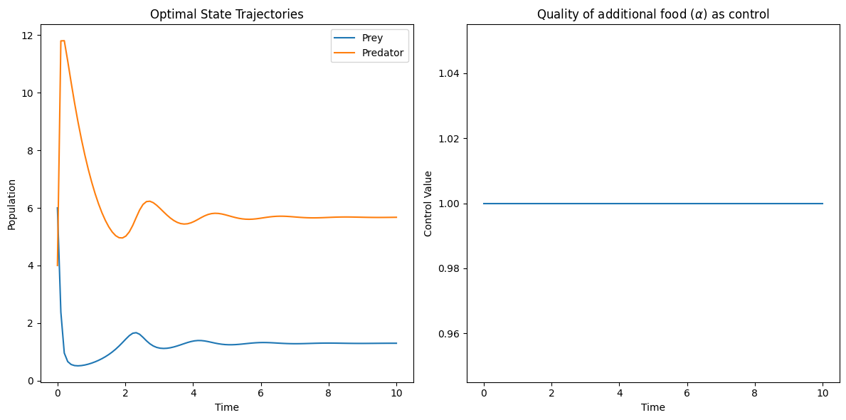
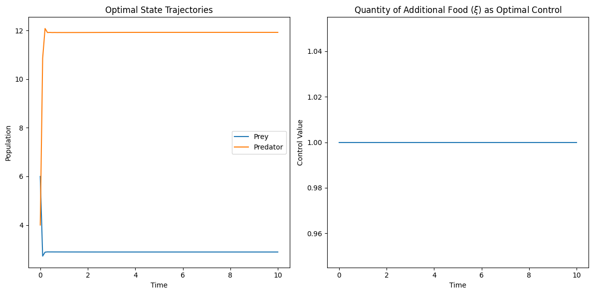
In this subsection, we simulated the time-optimal control problems 6 and 12 using python and driven the system to a prey-elimination state. Considering the pest as prey and the natural enemies as predators, the additional food provided to the predator will be the optimal control. For a chosen parameter values, we could show that the optimal control is of bang-bang control. This shows the importance of our work to the pest management by using biological control.

The subplots in figure 1, 2 depict the optimal state trajectories and optimal control trajectories for the time-optimal control problems 6 and 12 respectively. These unconstrained optimization problems are solved using the BFGS algorithm by choosing the following parameters for the problems 6 and 12. $r=2.5,\ \gamma=10,\ g=1.5,\ m=1,\ \delta=0.01,\ \alpha=12,\ \xi=0.7$ .

Refer to caption — Figure 1: This figure depicts the optimal state trajectories and the optimal control trajectories for the system (6).

4 Model Formulation

In this section, we consider the following deterministic additional food provided prey-predator model exhibiting Holling type-IV functional response and intra-specific competition among predators. The model is given by:

\begin{split}\frac{\mathrm{d}N(t)}{\mathrm{d}t}&=rN(t)\left(1-\frac{N(t)}{K}\right)-\Bigg{(}\frac{cN(t)}{(\alpha\eta A+a)(bN^{2}(t)+1)+N(t)}\Bigg{)}P(t)\\ \frac{\mathrm{d}P(t)}{\mathrm{d}t}&=e\Bigg{(}\frac{N(t)+\eta A(bN^{2}(t)+1)}{(\alpha\eta A+a)(bN^{2}(t)+1)+N(t)}\Bigg{)}P(t)-m_{1}P(t)-\delta P(t)^{2}\end{split}

(17)

The biological meaning for all the parameters involved in the system (17) are enlisted and described in Table 2. The detailed derivation of the functional response and the model can be found in [3]. In order to reduce the complexity, we now reduce the number of parameters in the model (17) by introducing the transformations $N=ax,\ P=\frac{ay}{c}$ . Then the system (17) gets transformed to:

\begin{split}\frac{\mathrm{d}x}{\mathrm{d}t}&=rx\Bigg{(}1-\frac{x}{\gamma}\Bigg{)}-\Bigg{(}\frac{xy}{(1+\alpha\xi)(\omega x^{2}+1)+x}\Bigg{)}\\ \frac{\mathrm{d}y}{\mathrm{d}t}&=e\Bigg{(}\frac{x+\xi(\omega x^{2}+1)}{(\alpha\xi+1)(\omega x^{2}+1)+x}\Bigg{)}y-m_{1}y-m_{2}y^{2}\end{split}

(18)

where $\gamma=\frac{K}{a},\ \xi=\frac{\eta A}{a},\ \omega=ba^{2}m_{2}=\frac{c}{a\delta}$ .

Parameter	Definition	Dimension
T	Time	time
N	Prey density	biomass
P	Predator density	biomass
A	Additional food	biomass
r	Prey intrinsic growth rate	time^-1
K	Prey carrying capacity	biomass
c	Maximum rate of predation	time^-1
e	Maximum growth rate of predator	time^-1
m₁	Predator mortality rate	time^-1
$\delta$	Death rate of predators due to intra-specific competition	biomass^-1 time^-1
$\alpha$	Quality of additional food for predators	Dimensionless
b	Group defence in prey	biomass^-2

Table 2: Description of variables and parameters present in the systems (17), (18)

Theorem 4.1.

(Existence and Uniqueness of solutions of (18)) The interior of the positive quadrant of the state space is invariant and all the solutions of the system (18) initiating in the interior of the positive quadrant are asymptotically bounded in the region $B$ defined by
$\textbf{B}=\left\{(x,y)\in\mathbb{R}^{2}_{+}:0\leq x\leq\gamma,\;0\leq x+\frac{1}{\beta}y\leq M\right\}$ , where $M=\frac{\gamma(r+\eta)^{2}}{4r\eta}+\frac{e(\frac{\xi}{1+\alpha\xi}+\frac{\eta-m_{1}}{e})^{2}}{4m_{2}\eta}$ and $\eta>0$ sufficiently small.

Proof.

Let us define $V=x+\frac{1}{e}y$ . Now for any $\eta>0$ , consider the ordinary differential equation

$\displaystyle\dfrac{dV}{dt}+\eta V$	$\displaystyle=$	$\displaystyle rx\Bigg{(}1-\frac{x}{\gamma}\Bigg{)}-\Bigg{(}\frac{xy}{(1+\alpha\xi)(\omega x^{2}+1)+x}\Bigg{)}+\Bigg{(}\frac{x+\xi(\omega x^{2}+1)}{(\alpha\xi+1)(\omega x^{2}+1)+x}\Bigg{)}y$
		$\displaystyle-\frac{m_{1}}{e}y-\frac{m_{2}}{e}y^{2}+\eta x+\frac{\eta}{e}y$
	$\displaystyle=$	$\displaystyle(r+\eta)x-\frac{r}{\gamma}x^{2}+\frac{\xi y}{1+\alpha\xi+\frac{x}{\omega x^{2}+1}}-\frac{m_{1}}{e}y+\frac{\eta}{e}y-\frac{m_{2}}{e}y^{2}$
	$\displaystyle<$	$\displaystyle(r+\eta)x-\frac{r}{\gamma}x^{2}+\frac{\xi}{1+\alpha\xi}y-\frac{m_{1}}{e}y+\frac{\eta}{e}y-\frac{m_{2}}{e}y^{2}$
	$\displaystyle=$	$\displaystyle(r+\eta)x-\frac{r}{\gamma}x^{2}+(\frac{\xi}{1+\alpha\xi}+\frac{\eta-m_{1}}{e})y-\frac{m_{2}}{e}y^{2}$

Since $Ax-Bx^{2}\leq\frac{A^{2}}{4B}$ , by choosing $\eta$ sufficiently small ( $\eta\ll\delta$ ), we get the relation

\dfrac{dV}{dt}+\eta V\leq\frac{\gamma(r+\eta)^{2}}{4r}+\frac{e(\frac{\xi}{1+\alpha\xi}+\frac{\eta-m_{1}}{e})^{2}}{4m_{2}}

Now, by choosing $M^{\prime}=\frac{\gamma(r+\eta)^{2}}{4r}+\frac{e(\frac{\xi}{1+\alpha\xi}+\frac{\eta-m_{1}}{e})^{2}}{4m_{2}}$ , we get

\dfrac{dV}{dt}+\eta V\leq M^{\prime}

(19)

0<V(t)<\frac{M^{\prime}}{\eta}(1-\exp(-\eta t))+\omega(0)\exp(-\eta t)

(20)

Now, from (20) we see that as $t$ becomes large enough, we get $0\leq V(t)\leq\frac{M^{\prime}}{\eta}$ . Let $M=\frac{M^{\prime}}{\eta}$ . Then, $0\leq V(t)\leq M$ . Hence, the solutions of the additional food provided system (18) with positive initial conditions $(x_{0},y_{0})$ will be within the set B. ∎

5 Time-Optimal Control Studies for Holling type-IV Systems

In this section, we formulate and characterise two time-optimal control problems with quality of additional food and quantity of additional food as control parameters respectively. We shall drive the system 18 from the initial state $(x_{0},y_{0})$ to the final state $(\bar{x},\bar{y})$ in minimum time.

5.1 Quality of Additional Food as Control Parameter

We assume that the quantity of additional food $(\xi)$ is constant and the quality of additional food varies in $[\alpha_{\text{min}},\alpha_{\text{max}}]$ . The time-optimal control problem with additional food provided prey-predator system involving Holling type-IV functional response and intra-specific competition among predators (18) with quality of additional food ( $\alpha$ ) as control parameter is given by

\begin{rcases}&\displaystyle{\bf{\min_{\alpha_{\min}\leq\alpha(t)\leq\alpha_{\max}}T}}\\ &\text{subject to:}\\ &\frac{\mathrm{d}x}{\mathrm{d}t}=rx\Big{(}1-\frac{x}{\gamma}\Big{)}-\Bigg{(}\frac{xy}{(1+\alpha\xi)(\omega x^{2}+1)+x}\Bigg{)}\\ &\frac{\mathrm{d}y}{\mathrm{d}t}=e\Bigg{(}\frac{x+\xi(\omega x^{2}+1)}{(\alpha\xi+1)(\omega x^{2}+1)+x}\Bigg{)}y-m_{1}y-m_{2}y^{2}\\ &(x(0),y(0))=(x_{0},y_{0})\ \text{and}\ (x(T),y(T))=(\bar{x},\bar{y}).\end{rcases}

(21)

This problem can be solved using a transformation on the independent variable $t$ by introducing an independent variable $s$ such that $\mathrm{d}t=((1+\alpha\xi)(\omega x^{2}+1)+x)\mathrm{d}s$ . This transformation converts the time-optimal control problem 21 into the following linear problem.

\begin{rcases}&\displaystyle{\bf{\min_{\alpha_{\min}\leq\alpha(t)\leq\alpha_{\max}}S}}\\ &\text{subject to:}\\ &\dot{x}(s)=rx(1-\frac{x}{\gamma})(x+(1+\omega x^{2})(1+\alpha\xi))-xy\\ &\dot{y}(s)=e(x+(1+\omega x^{2})\xi)y-(x+(1+\omega x^{2})(1+\alpha\xi))(m_{1}y+m_{2}y^{2})\\ &(x(0),y(0))=(x_{0},y_{0})\ \text{and}\ (x(S),y(S))=(\bar{x},\bar{y}).\end{rcases}

(22)

Hamiltonian function for this problem (22) is given by

\begin{split}\mathbb{H}(s,x,y,p,q)=&p(rx(1-\frac{x}{\gamma})(x+(1+\omega x^{2})(1+\alpha\xi))-xy)+q(e(x+(1+\omega x^{2})\xi)y\\ &-(x+(1+\omega x^{2})(1+\alpha\xi))(m_{1}y+m_{2}y^{2}))\\ =&\Big{[}prx(1-\frac{x}{\gamma})(1+\omega x^{2})\xi-q\xi(1+\omega x^{2})(m_{1}y+m_{2}y^{2})\Big{]}\alpha\\ &+\Big{[}p\Big{(}rx\Big{(}1-\frac{x}{\gamma}\Big{)}(x+1+\omega x^{2})-xy\Big{)}\\ &+q\Big{(}e(x+(1+\omega x^{2})\xi)y-(x+1+\omega x^{2})(m_{1}y+m_{2}y^{2})\Big{)}\Big{]}\\ \end{split}

Here, $p$ and $q$ are costate variables satisfying the adjoint equations

\begin{split}\dot{p}&=-p\Big{[}2rx^{2}\Big{(}1-\frac{x}{\gamma}\Big{)}-\frac{r}{\gamma}x(1+x^{2}+\alpha\xi)+r\Big{(}1-\frac{x}{\gamma}\Big{)}(1+x^{2}+\alpha\xi)-2xy\Big{]}-q\Big{[}2gxy-2x(my+\delta y^{2})\Big{]}\\ \dot{q}&=px^{2}-q\Big{[}g(x^{2}+\xi)-(1+x^{2}+\alpha\xi)(m+2\delta y)\Big{]}\end{split}

Since Hamiltonian is a linear function in $\alpha$ , the optimal control can be a combination of bang-bang and singular controls. Since we are minimizing the Hamiltonian, the optimal strategy is given by

\alpha^{*}(t)=\begin{cases}\alpha_{\max},&\text{ if }\frac{\partial\mathbb{H}}{\partial\alpha}<0\\ \alpha_{\min},&\text{ if }\frac{\partial\mathbb{H}}{\partial\alpha}>0\end{cases}

(23)

where

\frac{\partial\mathbb{H}}{\partial\alpha}=prx\Big{(}1-\frac{x}{\gamma}\Big{)}\xi-q\xi(my+\delta y^{2})

(24)

This problem 22 admits a singular solution if there exists an interval $[s_{1},s_{2}]$ on which $\frac{\partial\mathbb{H}}{\partial\alpha}=0$ . Therefore,

\frac{\partial\mathbb{H}}{\partial\alpha}=prx\Big{(}1-\frac{x}{\gamma}\Big{)}\xi-q\xi(my+\delta y^{2})=0\textit{ i.e. }\frac{p}{q}=\frac{\gamma(my+\delta y^{2})}{rx(x-\gamma)}

(25)

Differentiating $\frac{\partial\mathbb{H}}{\partial\alpha}$ with respect to $s$ we obtain

\begin{split}\frac{\mathrm{d}}{\mathrm{d}s}\frac{\partial\mathbb{H}}{\partial\alpha}=&\frac{\mathrm{d}}{\mathrm{d}s}\Big{[}prx\Big{(}1-\frac{x}{\gamma}\Big{)}\xi-q\xi(my+\delta y^{2})\Big{]}\\ =&r\xi x(1-\frac{x}{\gamma})\dot{p}+pr\xi(1-\frac{2x}{\gamma})\dot{x}-\xi(my+\delta y^{2})\dot{q}-q\xi(m+2\delta y)\dot{y}\end{split}

Substituting the values of $\dot{x},\dot{y},\dot{p},\dot{q}$ in the above equation, we obtain

\begin{split}\frac{\mathrm{d}}{\mathrm{d}s}\frac{\partial\mathbb{H}}{\partial\alpha}=&pr\Big{(}1-\frac{2x}{\gamma}\Big{)}\xi\Big{[}rx\Big{(}1-\frac{x}{\gamma}\Big{)}(1+x^{2}+\alpha\xi)-x^{2}y\Big{]}\\ &-q\xi(m+2\delta y)\Big{[}g(x^{2}+\xi)y-(1+x^{2}+\alpha\xi)(my+\delta y^{2})\Big{]}\\ &-\xi(my+\delta y^{2})\Big{[}px^{2}-q(g(x^{2}+\xi)-(1+x^{2}+\alpha\xi)(m+2\delta y))\Big{]}\\ &+rx\Big{(}1-\frac{x}{\gamma}\Big{)}\xi\Big{[}-p\Bigg{(}2rx^{2}\Big{(}1-\frac{x}{\gamma}\Big{)}-\frac{r}{\gamma}x(1+x^{2}+\alpha\xi)+r\Big{(}1-\frac{x}{\gamma}\Big{)}(1+x^{2}+\alpha\xi)-2xy\Bigg{)}\\ &-q(2gxy-2x(my+\delta y^{2}))\Big{]}\end{split}

Along the singular arc, $\frac{\mathrm{d}}{\mathrm{d}s}\frac{\partial\mathbb{H}}{\partial\alpha}=0$ . This implies that

\begin{split}pr\Big{(}1-\frac{2x}{\gamma}\Big{)}\xi\Big{[}rx\Big{(}1-\frac{x}{\gamma}\Big{)}(1+x^{2}+\alpha\xi)-x^{2}y\Big{]}&\\ -q\xi(m+2\delta y)\Big{[}g(x^{2}+\xi)y-(1+x^{2}+\alpha\xi)(my+\delta y^{2})\Big{]}&\\ -\xi(my+\delta y^{2})\Big{[}px^{2}-q(g(x^{2}+\xi)-(1+x^{2}+\alpha\xi)(m+2\delta y))\Big{]}&\\ +rx\Big{(}1-\frac{x}{\gamma}\Big{)}\xi\Big{[}-p\Bigg{(}2rx^{2}\Big{(}1-\frac{x}{\gamma}\Big{)}-\frac{r}{\gamma}x(1+x^{2}+\alpha\xi)+r\Big{(}1-\frac{x}{\gamma}\Big{)}(1+x^{2}+\alpha\xi)-2xy\Bigg{)}&\\ -q(2gxy-2x(my+\delta y^{2}))\Big{]}&=0\end{split}

and that

\frac{p}{q}=\frac{\gamma y(2grx^{2}(-\gamma+x)-\delta g\gamma(x^{2}+\xi)y+2r(\gamma-x)x^{2}(m+\delta y))}{x^{2}(2r^{2}(\gamma-x)^{2}x+\gamma^{2}(m-r)y+\delta\gamma^{2}y^{2})}

(26)

From 25 and 26, we have $\gamma y(\gamma^{2}xy(m+\delta y)(m-r+\delta y)+gr(\gamma-x)(2r(\gamma-x)x^{2}+\delta\gamma(x^{2}+\xi)y))=0$ . The solutions of this cubic equation gives the switching points of the bang-bang control.

5.2 Quantity of Additional Food as Control Parameter

We assume that the quality of additional food $(\alpha)$ is constant and the quantity of additional food varies in $[\xi_{\text{min}},\xi_{\text{max}}]$ . The time-optimal control problem with additional food provided prey-predator system involving Holling type-IV functional response and intra-specific competition among predators (18) with quantity of additional food ( $\xi$ ) as control parameter is given by

\begin{rcases}&\displaystyle{\bf{\min_{\xi_{\min}\leq\xi(t)\leq\xi_{\max}}T}}\\ &\text{subject to:}\\ &\dot{x}(t)=rx(t)\Big{(}1-\frac{x(t)}{\gamma}\Big{)}-\frac{x^{2}(t)y(t)}{1+x^{2}(t)+\alpha\xi}\\ &\dot{y}(t)=gy(t)\Big{(}\frac{x^{2}(t)+\xi}{1+x^{2}(t)+\alpha\xi}\Big{)}-my(t)-\delta y^{2}(t)\\ &(x(0),y(0))=(x_{0},y_{0})\ \text{and}\ (x(T),y(T))=(\bar{x},\bar{y}).\end{rcases}

(27)

\begin{rcases}&\displaystyle{\bf{\min_{\xi_{\min}\leq\xi(t)\leq\xi_{\max}}S}}\\ &\text{subject to:}\\ &\dot{x}(s)=rx(1-\frac{x}{\gamma})(1+x^{2}+\alpha\xi)-x^{2}y\\ &\dot{y}(s)=g(x^{2}+\xi)y-(1+x^{2}+\alpha\xi)(my+\delta y^{2})\\ &(x(0),y(0))=(x_{0},y_{0})\ \text{and}\ (x(S),y(S))=(\bar{x},\bar{y}).\end{rcases}

(28)

Hamiltonian function for this problem (28) is given by

\begin{split}\mathbb{H}(s,x,y,p,q)&=p\Big{[}rx(1-\frac{x}{\gamma})(1+x^{2}+\alpha\xi)-x^{2}y\Big{]}+q\Big{[}g(x^{2}+\xi)y-(1+x^{2}+\alpha\xi)(my+\delta y^{2})\Big{]}\\ &=\Big{[}prx(1-\frac{x}{\gamma})\xi-q\xi(my+\delta y^{2})\Big{]}\alpha\\ &+\Big{[}p(rx(1-\frac{x}{\gamma})(1+x^{2})-x^{2}y)+q(g(x^{2}+\xi)y-(1+x^{2})(my+\delta y^{2}))\Big{]}\\ \end{split}

Here, $p$ and $q$ are costate variables satisfying the adjoint equations

\begin{split}\dot{p}&=-p\Big{[}2rx^{2}(1-\frac{x}{\gamma})-\frac{rx(1+x^{2}+\alpha\xi)}{\gamma}+r(1-\frac{x}{\gamma})(1+x^{2}+\alpha\xi)-2xy\Big{]}-q\Big{[}2gxy-2x(my+\delta y^{2})\Big{]}\\ \dot{q}&=px^{2}-q\Big{[}g(x^{2}+\xi)-(1+x^{2}+\alpha\xi)(m+2\delta y)\Big{]}\end{split}

\xi^{*}(t)=\begin{cases}\xi_{\max},&\text{ if }\frac{\partial\mathbb{H}}{\partial\xi}<0\\ \xi_{\min},&\text{ if }\frac{\partial\mathbb{H}}{\partial\xi}>0\end{cases}

(29)

where

\frac{\partial\mathbb{H}}{\partial\xi}=prx(1-\frac{x}{\gamma})\xi-q\xi(my+\delta y^{2})

(30)

This problem 28 admits a singular solution if there exists an interval $[s_{1},s_{2}]$ on which $\frac{\partial\mathbb{H}}{\partial\xi}=0$ . Therefore,

\frac{\partial\mathbb{H}}{\partial\xi}=prx\Big{(}1-\frac{x}{\gamma}\Big{)}\xi-q\xi(my+\delta y^{2})=0\textit{ i.e. }\frac{p}{q}=\frac{\gamma(my+\delta y^{2})}{rx(x-\gamma)}

(31)

Differentiating $\frac{\partial\mathbb{H}}{\partial\xi}$ with respect to $s$ we obtain

\begin{split}\frac{\mathrm{d}}{\mathrm{d}s}\frac{\partial\mathbb{H}}{\partial\xi}&=\frac{\mathrm{d}}{\mathrm{d}s}\Big{[}prx\Big{(}1-\frac{x}{\gamma}\Big{)}\xi-q\xi(my+\delta y^{2})\Big{]}\\ &=r\xi x(1-\frac{x}{\gamma})\dot{p}+pr\xi(1-\frac{2x}{\gamma})\dot{x}-\xi(my+\delta y^{2})\dot{q}-q\xi(m+2\delta y)\dot{y}\end{split}

Substituting the values of $\dot{x},\dot{y},\dot{p},\dot{q}$ in the above equation, we obtain

\begin{split}\frac{\mathrm{d}}{\mathrm{d}s}\frac{\partial\mathbb{H}}{\partial\xi}=&pr\Big{(}1-\frac{2x}{\gamma}\Big{)}\xi\Big{(}rx\Big{(}1-\frac{x}{\gamma}\Big{)}(1+x^{2}+\alpha\xi)-x^{2}y\Big{)}\\ &-q\xi(m+2\delta y)\Big{(}g(x^{2}+\xi)y-(1+x^{2}+\alpha\xi)(my+\delta y^{2})\Big{)}\\ &-\xi(my+\delta y^{2})\Big{(}px^{2}-q(g(x^{2}+\xi)-(1+x^{2}+\alpha\xi)(m+2\delta y))\Big{)}\\ &+rx\Big{(}1-\frac{x}{\gamma}\Big{)}\xi\Bigg{(}-p\Big{(}2rx^{2}\Big{(}1-\frac{x}{\gamma}\Big{)}-\frac{rx(1+x^{2}+\alpha\xi)}{\gamma}+r(1-\frac{x}{\gamma})(1+x^{2}+\alpha\xi)-2xy\Big{)}\\ &-q(2gxy-2x(my+\delta y^{2}))\Bigg{)}\end{split}

Along the singular arc, $\frac{\mathrm{d}}{\mathrm{d}s}\frac{\partial\mathbb{H}}{\partial\xi}=0$ . This implies that

\begin{split}pr\Big{(}1-\frac{2x}{\gamma}\Big{)}\xi\Big{(}rx\Big{(}1-\frac{x}{\gamma}\Big{)}(1+x^{2}+\alpha\xi)-x^{2}y\Big{)}-q\xi(m+2\delta y)\Big{(}g(x^{2}+\xi)y-(1+x^{2}+\alpha\xi)(my+\delta y^{2})\Big{)}&\\ -\xi(my+\delta y^{2})\Big{(}px^{2}-q(g(x^{2}+\xi)-(1+x^{2}+\alpha\xi)(m+2\delta y))\Big{)}&\\ +rx\Big{(}1-\frac{x}{\gamma}\Big{)}\xi\Bigg{(}-p\Big{(}2rx^{2}\Big{(}1-\frac{x}{\gamma}\Big{)}-\frac{rx(1+x^{2}+\alpha\xi)}{\gamma}+r(1-\frac{x}{\gamma})(1+x^{2}+\alpha\xi)-2xy\Big{)}&\\ -q(2gxy-2x(my+\delta y^{2}))\Bigg{)}&=0\end{split}

and that

\frac{p}{q}=\frac{\gamma y(2grx^{2}(-\gamma+x)-\delta g\gamma(x^{2}+\xi)y+2r(\gamma-x)x^{2}(m+\delta y))}{x^{2}(2r^{2}(\gamma-x)^{2}x+\gamma^{2}(m-r)y+\delta\gamma^{2}y^{2})}

(32)

From 31 and 32, we have $\gamma y(\gamma^{2}xy(m+\delta y)(m-r+\delta y)+gr(\gamma-x)(2r(\gamma-x)x^{2}+\delta\gamma(x^{2}+\xi)y))=0$ . The solutions of this cubic equation gives the switching points of the bang-bang control.

5.3 Applications to Pest Management

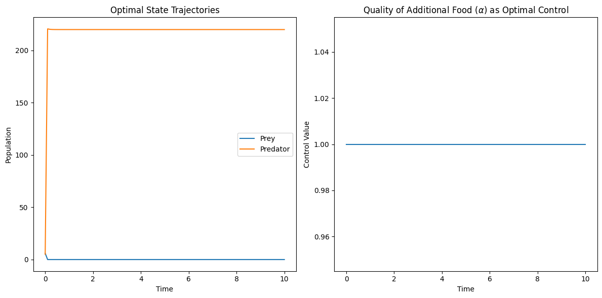
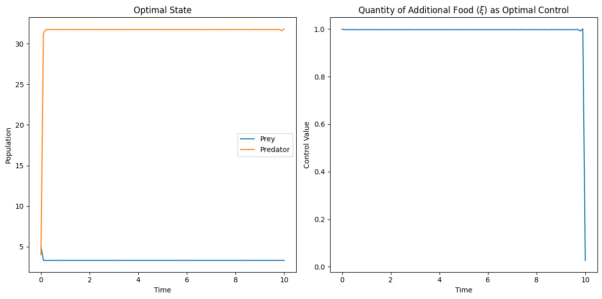
In this subsection, we simulated the time-optimal control problems 22 and 28 using python and driven the system to a prey-elimination state. Considering the pest as prey and the natural enemies as predators, the additional food provided to the predator will be the optimal control. For a chosen parameter values, we could show that the optimal control is of bang-bang control. This shows the importance of our work to the pest management by using biological control.

The subplots in figure 3, 4 depict the optimal state trajectories and optimal control trajectories for the time-optimal control problems 22 and 28 respectively. These unconstrained optimization problems are solved using the BFGS algorithm by choosing the following parameters for the problems 22 and 28. $r=2.5,\ \gamma=5,\ \omega=3,\ \xi=4,\ e=4,\ m_{1}=1,\ m_{2}=0.01$ .

6 Discussions and Conclusions

This paper studies two deterministic prey-predator systems exhibiting Holling type-III functional response and Holling type-IV functional responses respectively. We do the time-optimal control studies for these systems, with the quality and the quantity of additional food as control variables. To begin with, we formulated deterministic models by incorporating intra-specific competition among predators. In theorem 2.1, we proved the existence of a unique positive global solution of (2). In theorem 4.1, we proved the existence of a unique positive global solution of (18). Further, we formulated the time-optimal control problem with the objective to minimize the final time in which the system reaches the pre-defined state. Using the Pontraygin maximum principle, we characterized the optimal control values. We also numerically simulated the theoretical findings and applied them in the context of pest management.

Some of the salient features of this work include the following. This work captures the commonly observed intra-specific competition among predators implicitly in the context of models exhibiting Holling type-III and Holling type-IV functional responses. Also, this paper mainly deals with the novel study of the time-optimal control problems by transforming the independent variable in the control system. This work has been an initial attempt dealing with the Time Optimal Control studies for prey-predator systems involving intra-specific competition among predators. Since this is an initial exploratory research we didn’t include finer specificalities such as sensitivity analysis and also did not elaborate much on the bifurcation aspect. In future we wish to incorporate and study these aspects.

Financial Support:

This research was supported by National Board of Higher Mathematics(NBHM), Government of India(GoI) under project grant - Time Optimal Control and Bifurcation Analysis of Coupled Nonlinear Dynamical Systems with Applications to Pest Management,
Sanction number: (02011/11/2021NBHM(R.P)/R $\&$ D II/10074).

Conflict of Interests Statement:

The authors have no conflicts of interest to disclose.

Ethics Statement:

This research did not required ethical approval.

Acknowledgments

The authors dedicate this paper to the founder chancellor of SSSIHL, Bhagawan Sri Sathya Sai Baba. The corresponding author also dedicates this paper to his loving elder brother D. A. C. Prakash who still lives in his heart.

References

[1] Mark Kot “Elements of mathematical ecology” Cambridge University Press, 2001
[2] Johan A Metz and Odo Diekmann “The dynamics of physiologically structured populations” Springer, 2014
[3] P D N Srinivasu, D K K Vamsi and I Aditya “Biological conservation of living systems by providing additional food supplements in the presence of inhibitory effect: a theoretical study using predator–prey models” In Differential Equations and Dynamical Systems 26.1 Springer, 2018, pp. 213–246
[4] P D N Srinivasu, D K K Vamsi and V S Ananth “Additional food supplements as a tool for biological conservation of predator-prey systems involving type III functional response: A qualitative and quantitative investigation” In Journal of theoretical biology 455 Elsevier, 2018, pp. 303–318
[5] D K K Vamsi, Deva Siva Sai Murari Kanumoori and Bishal Chhetri “Additional food supplements as a tool for biological conservation of biosystems in the presence of inhibitory effect of the prey” In Acta biotheoretica 68.3 Springer, 2020, pp. 321–355
[6] V S Ananth and D K K Vamsi “Influence of quantity of additional food in achieving biological conservation and pest management in minimum-time for prey-predator systems involving Holling type III response” In Heliyon 7.8 Elsevier, 2021, pp. e07699
[7] V S Ananth and D K K Vamsi “Achieving Minimum-Time Biological Conservation and Pest Management for Additional Food provided Predator–Prey Systems involving Inhibitory Effect: A Qualitative Investigation” In Acta Biotheoretica 70.1 Springer, 2022, pp. 1–51
[8] V S Ananth and D K K Vamsi “An Optimal Control Study with Quantity of Additional food as Control in Prey-Predator Systems involving Inhibitory Effect” In Computational and Mathematical Biophysics 9.1 De Gruyter Open Access, 2021, pp. 114–145
[9] Daliparthi Bhanu Prakash and Dasu Krishna Kiran Vamsi “Stochastic optimal and time-optimal control studies for additional food provided prey–predator systems involving Holling type III functional response” In Computational and Mathematical Biophysics 11.1 De Gruyter, 2023, pp. 20220144
[10] D Bhanu Prakash and D K K Vamsi “Stochastic Time-Optimal Control and Sensitivity Studies for Additional Food provided Prey-Predator Systems involving Holling Type-IV Functional Response” In Frontiers in Applied Mathematics and Statistics 9 Frontiers, pp. 1122107
[11] Garrett Birkhoff and Gian-Carlo Rota “Ordinary differential equations” Ginn, 1962
[12] Lamberto Cesari “Optimization—theory and applications: problems with ordinary differential equations” Springer Science & Business Media, 2012