Tight and attainable quantum speed limit for open systems

Quantum speed limit (QSL) (or equivalently to call the quantum speed limit time (QSLT)) is an important feature of a dynamical system, which mainly characterizes the minimal time required for a state evolving to a target state. It is a constrained optimization problem important in quantum metrology [1, 2, 3], quantum optimal control [4, 5, 6, 7], quantum information processing [8, 9]. Recently, it’s considered a meaningful index for a given quantum system to evaluate its dynamics characteristics involving robustness [10], non-Markovianity [11, 12], upper bound of changing rate of expected value of observable [13], decoherence time [14, 15, 16, 17], interaction speed in spin system [18, 19] and changing rate of phase [20] and so on [21, 22]. Besides, the quantum speed limit is widely used to explore the intrinsic nature of physical systems, such as for the many-body system [23], ultracold atomic system [24], non-Hermitian system [25] and entanglement [26, 27, 28, 29, 30, 23]. For the application fields, studies of the quantum speed limit are involved in machine learning [31], quantum measurement [32] and thermometry [33].

QSL was first addressed for a unitary evolution from a pure state to its orthogonal state by Mandelstam and Tamm [34], who presented the famous time-Energy uncertainty (MT bound) $\tau_{MT}^{\bot}=\pi/(2\Delta E)$, where $(\Delta E)^{2}=\langle H^{2}\rangle-\langle H\rangle^{2}$ stands for the variance of Hamiltonian of the system [35]. Later, Margolus and Levitin [36] established another bound (ML bound) of the unitary evolution between pure orthogonal states as $\tau_{ML}^{\bot}=\pi/2E$ based on the average energy $E$ [35]. A tighter bound was obtained by the combination of MT and ML bounds as $\tau_{MT-ML}^{\bot}=\pi/(2\min\{E,\Delta E\})$ [37]. Giovannetti et al. generalized MT and ML bounds to the mixed initial state [38]. However, a deeper understanding of the QSL could count on the geometrical perspective first developed by Anandan and Aharanov for the MT bound with time-dependent Hamiltonian in terms of the Fubini-Study metric on the pure-state space [39]. Up to now, various geometrical distances have been exploited to develop QSL for density matrices [40, 41, 42, 43, 44, 45, 46, 47, 48, 35, 49, 50, 51, 52, 15, 13, 53, 54]. Considering the inevitable contact with environments, the QSL has also been developed for open system [55] based on different metrics such as quantum Fisher information [56], relative purity [51], and the MT bound and the ML bound have been extended to open systems in terms of a geometric way [57]. In addition, QSL is also characterized based on quantum resource theory [58]. It is even shown that the speed limit is not a unique phenomenon in quantum systems [59, 60]. Every QSL could have its significance in that it gives a potentially different understanding of the bound on the evolution time of a system. The most typical examples are the MT and ML QSLs which bound the evolution time by the fluctuation of energy and the average energy, respectively. In this sense, it is important to establish a distinguished QSL.

The tightness and the attainability are key aspects of a good QSL bound, which strongly depends on the different understanding perspectives of QSL [61, 62]. If the dynamics (Hamiltonian or Lindblad) is fixed, the QSLT bounds the minimum evolution time between a pair of states with a given ‘distance.’ If the state ‘distance’ is given, the tight QSL bound means that dynamics drive the given initial state to the final state with the minimum time. MT and ML bounds are attainable for a unitary evolution if the initial state is the equal-weight superposition of two eigenstates of the Hamiltonian with zero ground-state energy [36]. Ref. [46] generalized the tight bound for the unitary case to the mixed states, Ref. [63] verifies this bound is attainable for any dimension. Ref. [64] proposed a QSLT bound attainable for dephasing and depolarized channels. For a tight bound, many papers focus on combining different QSLs.

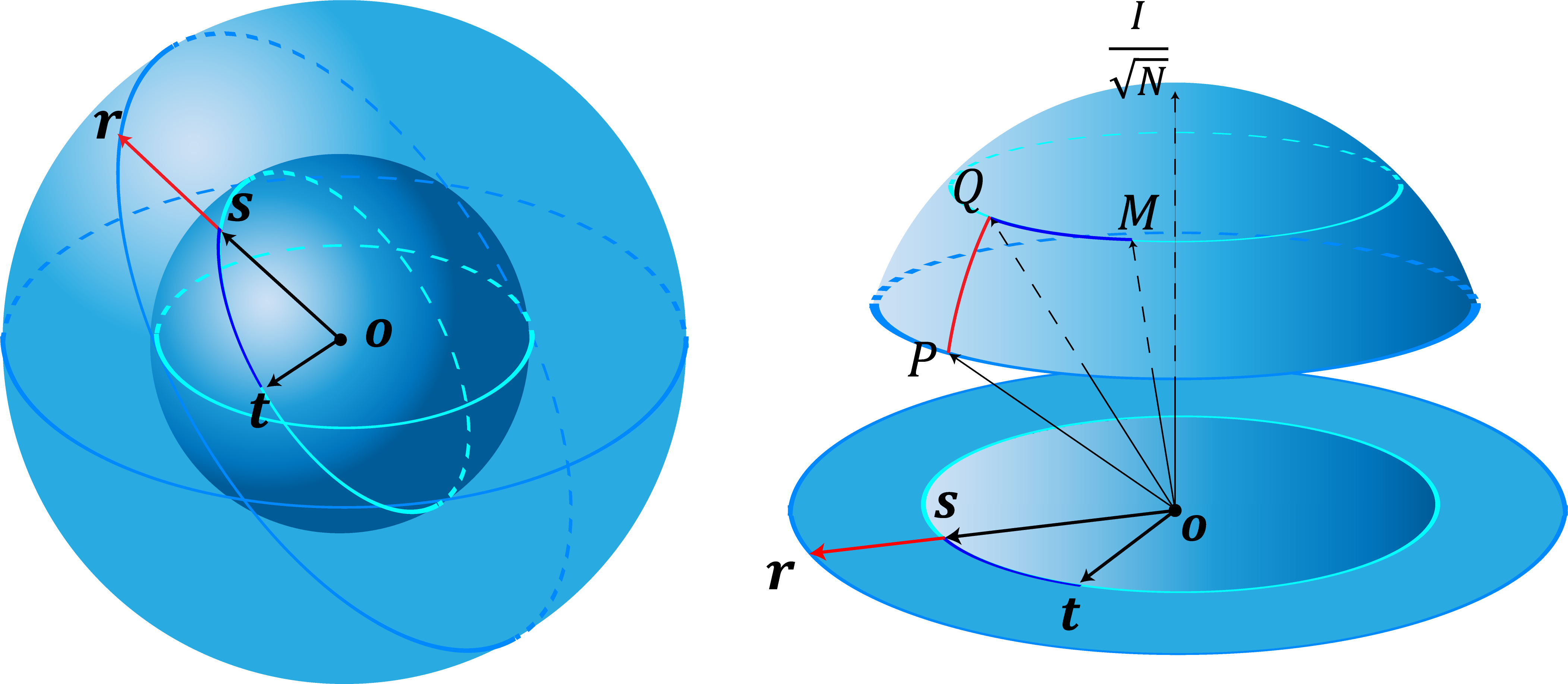
In this paper, we establish a tight and attainable QSLT for open systems in terms of a geometric approach. Similar to the Bloch representation of quantum states, we develop an intuitive geometric picture of quantum states. All the states are mapped to the surface of the high-dimensional sphere. In this picture, we derive a QSL for an open quantum system by a particularly-defined state distance. Our QSL is attainable in that for any given initial state, one can always find a dynamics to drive the initial state to the final state along the geodesic. In particular, we present a general condition for dynamics along the geodesic. The generalized amplitude damping dynamics and the dephasing dynamics evidence the attainability. In addition, we compare our QSL and the one in Ref. [64] by considering the unitary evolution of pure states and the particular amplitude damping dynamics. It is shown that our QSL is tight. In addition, numerical examples show that the QSLT of Ref. [64] is tighter than ours in many cases, which implies the combination of the two QSLs is necessary. The paper is organized as follows. We first propose the intuitive geometric picture of quantum states and present our QSL. Then we arrive at the general condition for dynamics along the geodesic, and then we give concrete examples to demonstrate the attainability of our QSL. Finally, we show the tightness of our QSL by comparing particular dynamics.

For an open system, the evolution of the quantum state $\rho_{t}$ is governed by the general master equation as

where $\mathcal{L}_{t}\left(\cdot\right)$ denotes a general dissipator of the system and the subscript $t$ indicates the potential dependence on time, in particular, we don’t specify whether $\mathcal{L}_{t}\left(\cdot\right)$ is Lindblad or not. Let $P_{t}=P\left(\rho_{t}\right)=\rho_{t}/\sqrt{Tr\rho_{t}^{2}}$, then for any pair of $P_{t}$ and $P_{t}^{\prime}$ we can define

based on the Hilbert-Schmidt distance $\langle P_{t},P_{t}^{\prime}\rangle=TrP_{t}^{{\dagger}}P_{t}^{\prime}$. Based on Schoeberg’s Theorem [65], which is firstly introduced by Ref. [66] to tackle with distance function equipped by the metric space consisted of density matrices, one can easily prove that $D(P_{t}||P_{t}^{\prime})$ is a good distance. Thus all $P_{t}$ can form a metric space $S\left(\mathcal{H}\right)$ with respect to the distance $D(P_{t}||P_{t}^{\prime})$. It is obvious that $D(P_{t}||P_{t}^{\prime})$ for a pair of density matrices $\rho$ and $\sigma$ can be explicitly written as

where $\mathcal{F}_{GM}(\rho,\sigma)=Tr\rho\sigma/(\sqrt{Tr\rho^{2}}\sqrt{Tr\sigma^{2}})$ is the alternative fidelity introduced in Ref. [67]. The alternative fidelity is also used in a different way for QSLT in Ref. [68].

To get the QSLT, we need the differential form of the distance $D(\rho||\sigma)$. Considering the infinitesimal evolution $\rho_{t}\longmapsto\rho_{t}+d\rho_{t}$, the distance reads

A direct deformation gives $\frac{Tr\rho_{t}(\rho_{t}+d\rho_{t})}{\sqrt{Tr\rho_{t}^{2}}\sqrt{Tr(\rho_{t}+d\rho_{t})^{2}}}=\cos ds=1-\frac{ds^{2}}{2}$, which indicates

Under the condition $d\rho_{t}\longmapsto 0$, we can expand $\frac{1}{\sqrt{Tr(\rho_{t}+d\rho_{t})^{2}}}$ to the second order:

Substituting Eq. (6) into Eq. (5), then we can immediately obtain the metric as

Denote $\mathcal{L}_{t}(P_{t})=\dot{\rho}_{t}/\sqrt{Tr\rho_{t}^{2}}$ if not confused(especially for the Lindbladian [69], a form of $\mathcal{L}_{t}(P_{t})$ is reasonable because $1/\sqrt{Tr\rho_{t}^{2}}$ is just a real number which is commutative with any operator), then the metric given in Eq. (7) turns to form of the Fubini-Study metric as

For infinitesimal $dt$, we have

According to $\dot{P}_{t}=\frac{P_{t+dt}-P_{t}}{dt}$, one can arrive at

Comparing Eq. (8) and Eq. (10), we have

In the above metric space, we can derive a speed limit based on the metric Eq. (10) and the distance Eq. (3) are as follows.

Theorem 1.-The minimal time for a given state $\rho_{0}$ to evolve to the state $\rho_{\tau}$ subject to the dynamics Eq. (1) is lower bounded by

with $P_{0}=\rho_{0}/\sqrt{Tr\rho_{0}^{2}}$ and $P_{\tau}=\rho_{\tau}/\sqrt{Tr\rho_{\tau}^{2}}$.

Proof.-Based on the distance, one can find that

which directly leads to $\tau\geq\tau_{qsl}$ as given in Eq. (12). $\square$

Now we’d like to give an intuitive understanding of the map between this metric space and the Bloch representation. As is given in Fig. 1. the states in the metric space form a spherical crown and are one-to-one mapped to the bottom surface of the hemispherical surface, which is geometrically the same as the circular section across the center of the Bloch sphere and the two points $\rho$ and $\sigma$. The apex of the the spherical crown is the maximally mixed state. The latitude of the bottom the surface of the spherical crown is determined by the intersection angle of a pure state and the maximally mixed state or the dimension of the state space. All the states of the same mixedness are distributed on the same latitude, which especially implies unitary evolution along the latitude. The evolution of purely reducing mixedness will undergo longitude. It can be noticed that for the evolution trajectories tracing geodesics in the Bloch sphere which is equipped by the Euclidean distance, it also traces a geodesics in our metric space.

Attainability.-It is easy to find that the quantum speed limit time $\tau_{qsl}$ is expressed by the distance $\arccos\langle P_{0},P_{\tau}\rangle$ divided by the average evolution speed $\left|\bar{v}_{t}\right|=\frac{1}{\tau}\int\nolimits_{0}^{\tau}\sqrt{\langle\dot{P}_{t},\dot{P}_{t}\rangle}dt$. Next, we will show that the QSL time presented in Theorem 1 can be attainable. Namely, given a distance and the average speed, one can always find a pair of quantum states and a corresponding dynamics such that the practical evolution time is exactly the QSL time.

Theorem 2.-The evolution of $\rho_{t}$ from a given initial state $\rho_{0}$ to a final state $\rho_{\tau}$ along the geodesic can be written as

and hence the geodesic is

where $\beta(t)$ is a monotonic function with $\beta(0)=0$ and $\beta(\tau)=1$.

The proof is given in Appendix A. Ref. [70] shows that the form of (14) can describe the behavior of atomic decay. It can be verified Eq. (15) is also the geodesics of the bound from Ref. [64]. In fact, one can easily verified that, the arbitrariness of $\beta_{t}$ and $\rho_{\tau}$ guarantee a highly freedom of form of the geodesics:

where $C$ is arbitrary traceless hermitian matrix.

Theorem 2 explicitly indicates the general form of the geodesic. In particular, $\rho_{\tau}=\frac{1}{N}$ corresponds to the longitude equation. Eq. (14) means the density matrix that evolves along a geodesic or the QSLT is attainable. However, it can be shown that bound (12) is impossible to be saturated for any unitary case by making a comparison to the bound $\tau_{\Phi}$ from Ref. [46]:

(17) derived from the monotone decreasing function $f(x)=\sqrt{2}arccosx-arccosx^{2}>f(1)=0$ when $0<x<1$.

Examples.-Considering an $N$-level system coupling to a heat bath with $b_{k}$ denoting the annihilator of its $k$th mode, the Hamiltonian for the total system is $H=\sum_{i=0}^{N}E_{i}\left|i\right\rangle\left\langle i\right|+\sum_{k}\omega_{k}b_{k}^{\dagger}b_{k}+\sum_{ik}(g_{k}\sigma_{+}^{i}b_{k}+h.c)$, where $E_{i}$ is the energy of $i$th energy level, and $\sigma_{-}^{i}=\left|0\right\rangle\left\langle i\right|$ and $\sigma_{+}^{i}=\left|i\right\rangle\left\langle 0\right|$ denote the transition operators. Following Ref. [71], one can obtain the dynamics for the reduced system as

where $s^{k}_{t}$ is the time-dependent Lamb shift and $\gamma^{k}_{t}$ represents the time-dependent decay rate. This equation describes the generalized amplitude dampling dynamics. Let the initial state be $\rho=\sum\limits_{i=0}\lambda_{i}\left|i\right\rangle\left\langle i\right|$ and suppose $\gamma^{k}_{t}\equiv\gamma_{t}$, the density matrix $\rho_{t}$ can be solved as

with $q_{t}=e^{-\int\nolimits_{0}^{t}\gamma_{t^{\prime}}dt^{\prime}}$. Derivation of $\rho_{t}$ in Eq. (19), we have $\dot{\rho_{t}}=\dot{q}_{t}\left(\sum\limits_{i}\lambda_{i}\left|i\right\rangle\left\langle i\right|\right)$, $\lambda_{0}=1-\sum\limits_{i\neq 0}\lambda_{i}$, which means the QSLT will be attainable due to theorem 2. To explicitly show it, let’s substitute Eq. (18) and Eq. (19) into Eq. (12), one can immediately find that in the duration $\tau$, the distance in terms of the average evolution speed is

where $c=\sqrt{\sum\limits_{i}\lambda_{i}^{2}}$, $b=\sum_{i\neq 0}\lambda_{i}$, $a=b^{2}+c^{2}$ and we suppose $q_{t}$ is monotonic. The distance away from the initial state $\rho_{0}$ is

with $f(q_{\tau})=\sqrt{1-2b|q_{\tau}|^{2}+a|q_{\tau}|^{2}}$ and $q_{0}=1$. It is easy to find that $D(\rho_{\tau}||\rho_{0})=\tau\bar{v}_{t}$, which directly shows the quantum speed limit time is consistent with the practical evolution time, $\tau_{qsl}=\frac{D(\rho_{\tau}||\rho_{0})}{\bar{v}_{t}}=\tau$.

The other attainable case is the dephasing dynamics. Suppose the above $N$-level system undergoes an environment consisting of multiple reservoirs with each two energy levels driven by an individual reservoir. Let the $j$th and the $k$th levels interact with the reservoir as $H_{jk}=\sum_{\nu}\sigma^{z}_{jk}(g_{\nu}b_{\nu}^{\dagger}+g_{\nu}^{*}b_{\nu})$, where $\sigma^{z}_{jk}=\left|j\right\rangle\left\langle j\right|-\left|k\right\rangle\left\langle k\right|$ for $j>k$, $g_{\nu}$ is the coupling strength, and $b_{\nu}$ is any operator of the reservoir corresponding to the $j$th and $k$th levels. Consider the time evolution of the system [71], for any initial state $\rho(0)$ one will get the final state as

where $V_{m}(t)$ is derived from the time-evolution operator performing on the state $\left|m\right\rangle$, and $\rho^{mn}_{B}(0)$ is the potential initial state of the reservoir corresponding to the $m$th and $n$th levels. Define the decay rates as

independent of $mn$, then the final state can be written as

The derivative of $\rho_{t}$ reads

It is evident that Eq. (25) has the same form as that in theorem 2, so the QSLT is attainable.

Again, let’s substitute Eq. (24) and Eq. (25) into Eq. (12), we can express the distance based on the average evolution speed as

where $R=\sqrt{\frac{\sum_{j\neq k}|\rho_{jk}|^{2}}{\sum_{i}\rho_{ii}^{2}}}$ and $\gamma_{t}$ is supposed to be monotonic. The distance away from the initial state is

with $F_{\tau}\left(k,s\right)=\sqrt{1+R^{k}e^{-s\gamma_{\tau}}}$. A further simplification can show that $D(\rho||\sigma)=\tau\bar{v}_{t}$, which means the QSL time $\tau_{qsl}=\frac{D(\rho||\sigma)}{\bar{v}_{t}}=\tau$.

At first, we would like to emphasize that in the two examples we choose the particular dynamics and the initial states to demonstrate the attainability. In fact, both the Hamiltonian and the initial states can change the attainability. In Appendix B, we present an example of qubit system to demonstrate the deviation of the evolution trajectory from the geodesic due to different Hamiltonian and initial states.

In addition, we don’t specify the explicit form of the decay rates except for monotonicity, the non-monotonicity or the divergence of $\gamma_{t}$ will force the evolution trajectory oscillates back and forth over the geodesics, and lead to $\tau_{qsl}<\tau$, namely, the evolution trajectory deviates from the geodesics. For example, if the decay rate takes

where $\delta=\sqrt{\lambda^{2}-2\gamma_{0}\lambda}$, and $\lambda$ and $\gamma_{0}$ represent the spectral width and coupling strength, respectively. If the parameter $\delta$ is real, i.e., $\gamma_{0}\leq\lambda/2$, the dynamics is Markovian, which implies a relatively weak coupling, and the decay rate can be taken as a constant $\gamma_{t}=\gamma_{0}$ for $\gamma_{0}\ll\lambda$. Conversely, if $\gamma_{0}\geq\lambda/2$, it means the stronger coupling described by the non-Markovian dynamics, which leads to non-monotonic $\gamma_{t}$. The evolution trajectory is not the geodesics, which is similar to the unsaturated effect of QSL bounds for the non-Markovian dynamics reported by the previous works [57, 12, 72].

The above two dynamics indicate the attainability of our QSL time in any dimensional state space. It is obvious that the farthest evolution is governed by the nonunitary dynamics instead of the unitary process. If we restrict the system to undergo the unitary evolution subject to the Hamiltonian $H_{t}$, the average speed $\bar{v}_{t}$ will be reduced to $\bar{v}_{t}=\frac{1}{\tau}\int\nolimits_{0}^{\tau}\sqrt{-\frac{1}{\hbar^{2}}Tr\{[P_{t},H_{t}]\}^{2}}dt$, which is the same as the speed $Q_{\Phi}$ in Ref. [46]. However, one can find that the effective distance $D(\rho||\sigma)$ is strictly larger than the distance $\Phi(\rho||\sigma)$ in Ref. [46] in nontrivial dynamics, so the practical evolution is strictly larger than our presented QSL time $\tau_{qsl}$. So our QSL cannot be attainable for a nontrivial unitary process.

Tightness.- Tightness is an important question in the QSL, which depends on not only the particular QSLT itself, but also the understanding of QSLT. For example, the MT and ML bounds for the unitary evolution can be the tightest, since they are obviously attainable for any pair of states as mentioned previously. Of course, if we understand the QSLT in the sense that for any given initial state whether one can find a proper dynamics to drive the state evolve along the geodesic, then our obtained QSLT is also the tightest since we have explicitly demonstrated the attainability. However, in the general sense, it is quite hard to evalute the tightness of a QSTL for open systems, because it is impossible to exhausted all the potential evolution trajectories to demonstrate the tightness of a single QSLT or to compare the inifinite QSLTs due to their dependence on the evolution trajectory. Therefore, we follows the usual and feasible comparison approach in the literature [73, 57, 51, 74, 64] namely, for given initial and final state, we compare two QSLTs subject to the same evolution trajectory.

Recently Ref. [64] has presented a tight QSLT

with good tightness based on the Euclidean distance $E(\rho_{0}||\rho_{\tau})=\sqrt{Tr(\rho_{0}-\rho_{\tau})^{2}}$. It has been shown that $\tau_{E}$ shares the same geodesic as our QSLT $\tau_{qsl}$. Here we would like to compare our QSLT with $\tau_{E}$.

Since $TrA^{2}TrB^{2}\geq(TrAB)^{2}$ for any Hermitian operators $A$ and $B$ [75], one can easily find

It is obvious that the left-hand side of the inequality (30) is the evolution speed of the bound $\tau_{E}$, and the right-hand side is the evolution speed of our bound. Because these two bounds are saturated by the same dynamics [41], integrating Eq. (30) one will immediately arrive at

When we restrict the unitary evolution and the pure initial state, the two sides of Eq. (30) are identical, but inequality in Eq. (31) still holds, which implies our bound shows $\tau_{qsl}>\tau_{E}$. In particular, the continuity of QSLT promises that for some evolution trajectories closed to the unitary path for the pure state, our bound still shows preferable tightness compared with $\tau_{E}$.

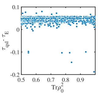
However, to demonstrate the tightness in general nonunitary cases, we sample $1000$ randomly generated dynamics process for qubit systems to calculate $\tau_{qsl}-\tau_{E}$ in Fig. 2. One can find that most of the given examples show our bound is tight, but some demonstrate $\tau_{E}$ is tighter than ours.

For an analytical demonstration, let’s consider a qubit interacting with a large bath. The Kraus operators are given as [41]

where $c$ is a parameter determined by the temperature of the bath and $p(t)$ is some increasing function of time $t$ describing the evolution path. Suppose the initial state $\rho_{0}=(1-\rho_{11}(0))\left|0\right\rangle\left\langle 0\right|+\rho_{10}(0)\left|0\right\rangle\left\langle 1\right|+\rho_{10}^{\ast}(0)\left|1\right\rangle\left\langle 0\right|+\rho_{11}(0)\left|1\right\rangle\left\langle 1\right|$, the density operator can be easily obtained as

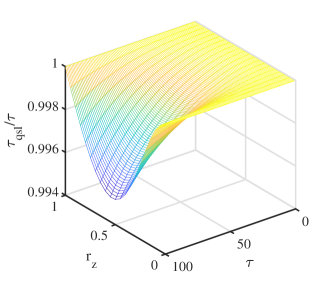
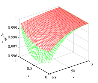
For the convenience of computation, we adopt the Bloch representation to describe the initial state $\rho_{11}=(1-r_{z})/2$ and $\rho_{10}$ is selected for ensuring the pure initial state. The ratio $\tau_{qsl}/\tau$ of QSL time to the actual evolution time is plotted in Fig. 3 (a), which indicates that the QSLT $\tau_{qsl}$ is less than the actual evolution time $\tau$ for most of the initial states, but is attainable if $\rho_{11}=0$ and $\rho_{11}=c$. In fact, one can find that $\rho_{11}=0$ or $c$ is the exact condition that can ensure $\dot{\rho}_{t}=\dot{\beta}(t)C$, where $C$ is time-independent, which is also the equivalent condition of geodesics dynamics. Additionally, we compare our QSLT with that proposed in Ref. [64] by the ratio $\tau_{qsl}/\tau$ in Fig. 3 (b). It is obvious that our QSLT is larger (tighter) than the QSLT in Ref. [64] .

Since the combination approach has been widely used in establishing tighter QSLT [57], combining the different QSLs could provide a tighter bound for the evolution time. Namely, a combination QSLT form as $\tau_{qsl}^{comb}=\left\{\tau_{qsl},\tau_{E}\right\}$ should be a good QSLT for an open system.

We have established a quantum speed limit for the open system by an intuitive geometrical picture. For any initial state, one can always find corresponding dynamics to achieve the ”fastest” evolution along the geodesic. We found the general condition for dynamics to saturate our QSL. By evidence, we consider the evolutions of a quantum state undergoing the generalized amplitude damping channel and the dephasing channel, which verify the attainability of our QSL when the decay rates are monotonic. But for the dynamics with the non-monotonic decay rate, such as the case of non-Markovian dynamics, the bound is unsaturated. We compare our QSLT with the tight one $\tau_{E}$ presented in Ref. [64]. We show our bound is tighter than $\tau_{E}$ for pure initial state governed by unitary (or close to unitary) evolution. Besides, we sample $1000$ non-unitary dynamics for qubit systems, and find that for most cases our bound is tighter than t$\tau_{E}$, but for some other cases the result is contrary, which implies the combination of the two QSLTs should be a tighter bound. In summary, we have presented attainable bound for QSLT, which provide a different understanding of QSLT.

This work was supported by the National Natural Science Foundation of China under Grants No.12175029, No. 12011530014 and No.11775040.

In this section, we show a proof to verify that Eq. (14) is the geodesics. Let $\Delta\rho_{\tau 0}=\rho_{\tau}-\rho_{0}$, then $\rho_{t}$ can be rewritten as $\rho_{t}=\rho_{0}+\beta(t)\Delta\rho_{\tau 0}.$ The derivation of $\rho_{t}$ reads $\dot{\rho}_{t}=\dot{\beta}(t)\left(\rho_{\tau}-\rho_{0}\right)$, which is exactly the equation (14). Solving the differential equation (14), one will obtain Eq. (15).

We will show that Eq. (14) is the geodesic. One can easily find

so the average evolution speed can be calculated as

where $\dot{\beta}(t)>0$ is considered since $\beta(t)$ is a monotonic function with $\beta(0)=0$ and $\beta(\tau)=1$. The evolution path is

A simple calculation can show that $\cos\int_{0}^{\tau}\left|v_{t}\right|dt=Tr\rho_{0}\rho_{\tau}/(\sqrt{Tr\rho_{0}^{2}}\sqrt{Tr\rho_{\tau}^{2}})$, which means Eq. (15) is the geodesic. The proof is finished. $\square$

Here we provide an example to illustrate that the system Hamiltonian can drive the evolution trajectory to deviate from the geodesics. Consider the master equation (18) in the Schrödinger picture as

where $\gamma$ is the time-independent decay rate, $\Sigma_{\pm}=U\sigma_{\pm}U^{\dagger}$ with $U=\cos\frac{\theta}{2}I-i\sin\frac{\theta}{2}\sigma_{y}$, $H_{\theta}$ is the parameter $\theta$ determined Hamiltonian with the eigenfrequency of $\Omega_{L}=\sqrt{\epsilon^{2}+\Omega^{2}}$, and $\epsilon$ and $\Omega$ denote the energy level difference and tunneling coupling, respectively. The solution of Eq. (37) is presented in Ref. [76] as

with

According to Eq. (16), the geodesics dynamics can be expressed as a product of real time-dependent factor and a time-independent hermitian matrix with zero-trace, hence the time-dependent imaginary factor of the non-diagonal entries should be vanish, it means that $r_{y}=0$, i.e., $r_{y}(0)=0$, $r_{x}(0)=r_{z}(0)$, $\theta=\pi/4$, one can immediately obtain that Eq. (38) is the geodesics due to $r_{x}(t)=r_{y}(t)$, and $[H_{\theta},\rho_{t}]=0$. That is, for this model, the system Hamiltonian drives the evolution trajectory deviate the geodesics except for the case when $\rho_{t}$ is commutative with the Hamiltonian. In the general cases, the presence of the time-dependent imaginary factor of the non-diagonal entries of the dynamics matrix always lead to a non-geodesics evolution.

References

- Giovannetti et al. [2011] V. Giovannetti, S. Lloyd, and L. Maccone, Advances in quantum metrology, Nature photonics 5, 222 (2011).
- Giovannetti et al. [2006] V. Giovannetti, S. Lloyd, and L. Maccone, Quantum metrology, Phys. Rev. Lett. 96, 010401 (2006).
- Chin et al. [2012] A. W. Chin, S. F. Huelga, and M. B. Plenio, Quantum metrology in non-markovian environments, Phys. Rev. Lett. 109, 233601 (2012).
- Caneva et al. [2009] T. Caneva, M. Murphy, T. Calarco, R. Fazio, S. Montangero, V. Giovannetti, and G. E. Santoro, Optimal control at the quantum speed limit, Phys. Rev. Lett. 103, 240501 (2009).
- Govenius et al. [2016] J. Govenius, R. E. Lake, K. Y. Tan, and M. Möttönen, Detection of zeptojoule microwave pulses using electrothermal feedback in proximity-induced josephson junctions, Phys. Rev. Lett. 117, 030802 (2016).
- Machnes et al. [2011] S. Machnes, U. Sander, S. J. Glaser, P. de Fouquières, A. Gruslys, S. Schirmer, and T. Schulte-Herbrüggen, Comparing, optimizing, and benchmarking quantum-control algorithms in a unifying programming framework, Phys. Rev. A 84, 022305 (2011).
- Poggi et al. [2013] P. M. Poggi, F. C. Lombardo, and D. A. Wisniacki, Quantum speed limit and optimal evolution time in a two-level system, Europhysics Letters 104, 40005 (2013).
- Girolami [2019] D. Girolami, How difficult is it to prepare a quantum state?, Phys. Rev. Lett. 122, 010505 (2019).
- Deffner [2020] S. Deffner, Quantum speed limits and the maximal rate of information production, Phys. Rev. Res. 2, 013161 (2020).
- Kobayashi and Yamamoto [2020] K. Kobayashi and N. Yamamoto, Quantum speed limit for robust state characterization and engineering, Phys. Rev. A 102, 042606 (2020).
- Zhang et al. [2015] Y.-J. Zhang, W. Han, Y.-J. Xia, J.-P. Cao, and H. Fan, Classical-driving-assisted quantum speed-up, Phys. Rev. A 91, 032112 (2015).
- Liu et al. [2016] H.-B. Liu, W. L. Yang, J.-H. An, and Z.-Y. Xu, Mechanism for quantum speedup in open quantum systems, Phys. Rev. A 93, 020105 (2016).
- García-Pintos et al. [2022] L. P. García-Pintos, S. B. Nicholson, J. R. Green, A. del Campo, and A. V. Gorshkov, Unifying quantum and classical speed limits on observables, Phys. Rev. X 12, 011038 (2022).
- Pires et al. [2016a] D. P. Pires, M. Cianciaruso, L. C. Céleri, G. Adesso, and D. O. Soares-Pinto, Generalized geometric quantum speed limits, Phys. Rev. X 6, 021031 (2016a).
- Marvian et al. [2016] I. Marvian, R. W. Spekkens, and P. Zanardi, Quantum speed limits, coherence, and asymmetry, Phys. Rev. A 93, 052331 (2016).
- Chenu et al. [2017] A. Chenu, M. Beau, J. Cao, and A. del Campo, Quantum simulation of generic many-body open system dynamics using classical noise, Phys. Rev. Lett. 118, 140403 (2017).
- Beau et al. [2017] M. Beau, J. Kiukas, I. L. Egusquiza, and A. del Campo, Nonexponential quantum decay under environmental decoherence, Phys. Rev. Lett. 119, 130401 (2017).
- Hamma et al. [2009] A. Hamma, F. Markopoulou, I. Prémont-Schwarz, and S. Severini, Lieb-robinson bounds and the speed of light from topological order, Phys. Rev. Lett. 102, 017204 (2009).
- Sawyer [2004] R. F. Sawyer, Evolution speed in some coupled-spin models, Phys. Rev. A 70, 022308 (2004).
- Sun et al. [2021] S.-N. Sun, Y.-G. Peng, X.-H. Hu, and Y.-J. Zheng, Quantum speed limit quantified by the changing rate of phase, Phys. Rev. Lett. 127, 100404 (2021).
- [21] G. N. Fleming, Unitarity bound on the evolution of nonstationary states, Nuovo Cim., A, v. 16A, no. 2, pp. 232-240 10.1007/BF02819419.
- Pires et al. [2021] D. P. Pires, K. Modi, and L. C. Céleri, Bounding generalized relative entropies: Nonasymptotic quantum speed limits, Phys. Rev. E 103, 032105 (2021).
- Bukov et al. [2019] M. Bukov, D. Sels, and A. Polkovnikov, Geometric speed limit of accessible many-body state preparation, Phys. Rev. X 9, 011034 (2019).
- del Campo [2021] A. del Campo, Probing quantum speed limits with ultracold gases, Phys. Rev. Lett. 126, 180603 (2021).
- Cui and Zheng [2012] X.-D. Cui and Y.-J. Zheng, Geometric phases in non-hermitian quantum mechanics, Phys. Rev. A 86, 064104 (2012).
- Liu et al. [2015] C. Liu, Z.-Y. Xu, and S.-Q. Zhu, Quantum-speed-limit time for multiqubit open systems, Phys. Rev. A 91, 022102 (2015).
- Kupferman and Reznik [2008] J. Kupferman and B. Reznik, Entanglement and the speed of evolution in mixed states, Phys. Rev. A 78, 042305 (2008).
- Xu et al. [2014] Z.-Y. Xu, S.-L. Luo, W. L. Yang, C. Liu, and S.-Q. Zhu, Quantum speedup in a memory environment, Phys. Rev. A 89, 012307 (2014).
- Zander et al. [2007] C. Zander, A. R. Plastino, A. Plastino, and M. Casas, Entanglement and the speed of evolution of multi-partite quantum systems, Journal of Physics A: Mathematical and Theoretical 40, 2861 (2007).
- Wu et al. [2014] S.-X. Wu, Y. Zhang, C.-S. Yu, and H.-S. Song, The initial-state dependence of the quantum speed limit, Journal of Physics A: Mathematical and Theoretical 48, 045301 (2014).
- Zhang et al. [2018] X.-M. Zhang, Z.-W. Cui, X. Wang, and M.-H. Yung, Automatic spin-chain learning to explore the quantum speed limit, Phys. Rev. A 97, 052333 (2018).
- García-Pintos and del Campo [2019] L. P. García-Pintos and A. del Campo, Quantum speed limits under continuous quantum measurements, New Journal of Physics 21, 033012 (2019).
- Campbell et al. [2018] S. Campbell, M. G. Genoni, and S. Deffner, Precision thermometry and the quantum speed limit, Quantum Science and Technology 3, 025002 (2018).
- Mandelstam and Tamm [1991] L. Mandelstam and I. Tamm, The uncertainty relation between energy and time in non-relativistic quantum mechanics, in Selected Papers, edited by B. M. Bolotovskii, V. Y. Frenkel, and R. Peierls (Springer Berlin Heidelberg, Berlin, Heidelberg, 1991) pp. 115–123.
- Deffner and Lutz [2013a] S. Deffner and E. Lutz, Energy–time uncertainty relation for driven quantum systems, Journal of Physics A: Mathematical and Theoretical 46, 335302 (2013a).
- Margolus and Levitin [1998] N. Margolus and L. B. Levitin, The maximum speed of dynamical evolution, Physica D: Nonlinear Phenomena 120, 188 (1998), proceedings of the Fourth Workshop on Physics and Consumption.
- Giovannetti et al. [2004] V. Giovannetti, S. Lloyd, and L. Maccone, The speed limit of quantum unitary evolution, Journal of Optics B: Quantum and Semiclassical Optics 6, S807 (2004).
- Giovannetti et al. [2003] V. Giovannetti, S. Lloyd, and L. Maccone, Quantum limits to dynamical evolution, Phys. Rev. A 67, 052109 (2003).
- Anandan and Aharonov [1990] J. Anandan and Y. Aharonov, Geometry of quantum evolution, Phys. Rev. Lett. 65, 1697 (1990).
- Russell and Stepney [2014] B. Russell and S. Stepney, A geometrical derivation of a family of quantum speed limit results (2014), arXiv:1410.3209 [quant-ph] .
- O’Connor et al. [2021] E. O’Connor, G. Guarnieri, and S. Campbell, Action quantum speed limits, Phys. Rev. A 103, 022210 (2021).
- Ektesabi et al. [2017] A. Ektesabi, N. Behzadi, and E. Faizi, Improved bound for quantum-speed-limit time in open quantum systems by introducing an alternative fidelity, Phys. Rev. A 95, 022115 (2017).
- Mondal et al. [2016] D. Mondal, C. Datta, and S. Sazim, Quantum coherence sets the quantum speed limit for mixed states, Physics Letters A 380, 689 (2016).
- Cai and Zheng [2017] X.-J. Cai and Y.-J. Zheng, Quantum dynamical speedup in a nonequilibrium environment, Phys. Rev. A 95, 052104 (2017).
- Wu and Yu [2018] S.-X. Wu and C.-S. Yu, Quantum speed limit for a mixed initial state, Phys. Rev. A 98, 042132 (2018).
- Campaioli et al. [2018] F. Campaioli, F. A. Pollock, F. C. Binder, and K. Modi, Tightening quantum speed limits for almost all states, Phys. Rev. Lett. 120, 060409 (2018).
- Zhang et al. [2014] Y.-J. Zhang, W. Han, Y.-J. Xia, J.-P. Cao, and H. Fan, Quantum speed limit for arbitrary initial states, Scientific reports 4, 1 (2014).
- Mondal and Pati [2016] D. Mondal and A. K. Pati, Quantum speed limit for mixed states using an experimentally realizable metric, Physics Letters A 380, 1395 (2016).
- Ness et al. [2022] G. Ness, A. Alberti, and Y. Sagi, Quantum speed limit for states with a bounded energy spectrum, Phys. Rev. Lett. 129, 140403 (2022).
- Andersson and Heydari [2014] O. Andersson and H. Heydari, Quantum speed limits and optimal hamiltonians for driven systems in mixed states, Journal of Physics A: Mathematical and Theoretical 47, 215301 (2014).
- del Campo et al. [2013] A. del Campo, I. L. Egusquiza, M. B. Plenio, and S. F. Huelga, Quantum speed limits in open system dynamics, Phys. Rev. Lett. 110, 050403 (2013).
- Sun et al. [2015a] Z. Sun, J. Liu, J. Ma, and X.-G. Wang, Quantum speed limits in open systems: Non-markovian dynamics without rotating-wave approximation, Scientific reports 5, 1 (2015a).
- Sun and Zheng [2019] S.-N. Sun and Y.-J. Zheng, Distinct bound of the quantum speed limit via the gauge invariant distance, Phys. Rev. Lett. 123, 180403 (2019).
- Zwierz [2012] M. Zwierz, Comment on “geometric derivation of the quantum speed limit”, Phys. Rev. A 86, 016101 (2012).
- Lidar et al. [2008] D. A. Lidar, P. Zanardi, and K. Khodjasteh, Distance bounds on quantum dynamics, Phys. Rev. A 78, 012308 (2008).
- Taddei et al. [2013] M. M. Taddei, B. M. Escher, L. Davidovich, and R. L. de Matos Filho, Quantum speed limit for physical processes, Phys. Rev. Lett. 110, 050402 (2013).
- Deffner and Lutz [2013b] S. Deffner and E. Lutz, Quantum speed limit for non-markovian dynamics, Phys. Rev. Lett. 111, 010402 (2013b).
- Campaioli et al. [2022] F. Campaioli, C.-S. Yu, F. A. Pollock, and K. Modi, Resource speed limits: maximal rate of resource variation, New Journal of Physics 24, 065001 (2022).
- Okuyama and Ohzeki [2018] M. Okuyama and M. Ohzeki, Quantum speed limit is not quantum, Phys. Rev. Lett. 120, 070402 (2018).
- Shanahan et al. [2018] B. Shanahan, A. Chenu, N. Margolus, and A. del Campo, Quantum speed limits across the quantum-to-classical transition, Phys. Rev. Lett. 120, 070401 (2018).
- Frey [2016] M. R. Frey, Quantum speed limits—primer, perspectives, and potential future directions, Quantum Information Processing 15, 3919 (2016).
- Deffner and Campbell [2017] S. Deffner and S. Campbell, Quantum speed limits: from heisenberg’s uncertainty principle to optimal quantum control, Journal of Physics A: Mathematical and Theoretical 50, 453001 (2017).
- Shao et al. [2020] Y.-Y. Shao, B. Liu, M. Zhang, H.-D. Yuan, and J. Liu, Operational definition of a quantum speed limit, Physical Review Research 2, 023299 (2020).
- Campaioli et al. [2019] F. Campaioli, F. A. Pollock, and K. Modi, Tight, robust, and feasible quantum speed limits for open dynamics, Quantum 3, 168 (2019).
- Schoenberg [1938] I. Schoenberg, Metric spaces and positive definite functions, Transactions of the American Mathematical Society 44, 522 (1938).
- Mendonça et al. [2008] P. E. M. F. Mendonça, R. d. J. Napolitano, M. A. Marchiolli, C. J. Foster, and Y.-C. Liang, Alternative fidelity measure between quantum states, Phys. Rev. A 78, 052330 (2008).
- Wang et al. [2008] X.-G. Wang, C.-S. Yu, and X. Yi, An alternative quantum fidelity for mixed states of qudits, Physics Letters A 373, 58 (2008).
- Poggi et al. [2021] P. M. Poggi, S. Campbell, and S. Deffner, Diverging quantum speed limits: A herald of classicality, PRX Quantum 2, 040349 (2021).
- Manzano [2020] D. Manzano, A short introduction to the Lindblad master equation, AIP Advances 10, 10.1063/1.5115323 (2020), 025106, https://pubs.aip.org/aip/adv/article-pdf/doi/10.1063/1.5115323/12881278/025106_1_online.pdf .
- Singh [1982] S. Singh, Field statistics in some generalized jaynes-cummings models, Phys. Rev. A 25, 3206 (1982).
- Breuer et al. [2002] H.-P. Breuer, F. Petruccione, et al., The theory of open quantum systems (Oxford University Press on Demand, 2002).
- Cianciaruso et al. [2017] M. Cianciaruso, S. Maniscalco, and G. Adesso, Role of non-markovianity and backflow of information in the speed of quantum evolution, Phys. Rev. A 96, 012105 (2017).
- Pires et al. [2016b] D. P. Pires, M. Cianciaruso, L. C. Céleri, G. Adesso, and D. O. Soares-Pinto, Generalized geometric quantum speed limits, Phys. Rev. X 6, 021031 (2016b).
- Sun et al. [2015b] Z. Sun, J. Liu, J. Ma, and X.-G. Wang, Quantum speed limits in open systems: Non-markovian dynamics without rotating-wave approximation, Scientific reports 5, 1 (2015b).
- Jin and Zhou [2015] L. Jin and Q. Zhou, Generalization of fan-todd inequality in the matrix theory, Journal of Anqing Normal University (Natural Science Edition) 21, 453001 (2015).
- Lan et al. [2022] K. Lan, S. Xie, and X. Cai, Geometric quantum speed limits for markovian dynamics in open quantum systems, New Journal of Physics 24, 055003 (2022).