


Illustrations of eight thunderstorm systems: tropical thunderstorms, winter thunderstorm, atmospheric river, single-cell, multi-cell, squall line, and supercell. Each image represents a unique thunderstorm system observed in meteorological studies.
Thunderscapes: Simulating the Dynamics of Mesoscale Convective System
Abstract.
A Mesoscale Convective System (MCS) is a collection of thunderstorms that function as a system, representing a widely discussed phenomenon in both the natural sciences and visual effects industries, and embodying the untamed forces of nature.In this paper, we present the first efficient, physically based mesoscale thunderstorms simulation model that integrates Grabowski-style cloud microphysics with hydrometeor electrification processes. Our model simulates thunderclouds development and lightning flashes within a unified meteorological framework, providing a realistic and efficient approach for graphical applications. By incorporating key physical principles, it effectively links cloud formation, electrification, and lightning generation. The simulation also encompasses various thunderstorm types and their corresponding lightning activities. For more details, see the dynamic video: Thunderscapes Video.
1. INTRODUCTION
Thunderstorms represent the wild power of nature and are a common atmospheric element in visual effects (VFX) industry. Notable works, such as Horizon Forbidden West: Burning Shores and Ghost of Tsushima(see Figure 2), demonstrate the importance of realistic atmospheric effects. Modern applications demand tools for efficient and realistic simulation of thunderstorms. However, current general purpose VFX software, such as Houdini and Maya, lacks standardized toolkits specifically designed for creating atmospheric phenomena like thunderstorms.

A scenic image from the video game Ghost of Tsushima showing dramatic landscapes and warrior scenes.

A scene from the video game Horizon Forbidden West: Burning Shores, showcasing futuristic landscapes and action.
Recent advances in computer graphics research have increasingly focused on cloud dynamics, incorporating atmospheric microphysical processes (Hädrich et al., 2020; Herrera et al., 2021; Amador Herrera et al., 2024). However, the critical role of atmospheric electrification in cloud development remains underexplored. This study aims to address this gap by integrating the electrification process, thus enhancing the consistency and realism of phenomena observed during thunderstorm events.
This paper presents an efficient, physically based method for simulating thunderstorm development. By coupling cloud microphysics with atmospheric hydrometeor electrification, our approach captures essential processes that contribute to the consistent formation of mesoscale thunderstorm phenomena.
The key contributions include:
-
(1)
We present a comprehensive framework for computing thunderstorm microphysics in the atmosphere, incorporating the transport of cloud hydrometeors and their electrification processes.
-
(2)
We introduce a lightweight parameterization that enables users to efficiently simulate various types of thunderstorms, along with their corresponding lightning effects.
-
(3)
We validate our simulation using different meteorological datasets to ensure the generation of physically credible and visually accurate atmospheric effects.
2. RELATED WORK
2.1. Simulating Thunderstorms in Computer Graphics
The simulation of atmospheric phenomena such as thunderstorms has been extensively explored through a variety of computational methods. Webanck et al. (Webanck et al., 2018) proposed a procedural approach for generating cloudscapes, while Miyazaki et al. (Miyazaki et al., 2002) simulated cumulus clouds by coupling computational fluid dynamics (CFD) with fundamental water transport equations. Ferreira et al. (Ferreira Barbosa et al., 2015) and Zhang et al. (Zhang et al., 2020) utilized position-based fluids (PBF) for adaptive cloud simulations. Smoothed Particle Hydrodynamics (SPH) techniques, as demonstrated by Goswami and Neyret (Goswami and Neyret, 2017), focus on real-time simulations of convective clouds. Additionally, Vimont et al. (Vimont et al., 2020) proposed a hybrid, 2D-layered atmospheric model to simulate mesoscale skyscapes.
Some studies have specifically focused on the simulation of volcanic cloud dynamics. Lastic et al. (Lastic et al., 2022) employed Lagrangian dynamics to simulate volcanic plumes and pyroclastic flows, while Pretorius et al. (Pretorius et al., 2024) integrated volcanic eruptions with atmospheric simulations to produce coherent skyscapes.
In the domain of lightning simulation, Reed and Wyvill (Reed and Wyvill, 1994), Kim and Lin (Kim and Lin, 2007), and Yun et al. (Yun et al., 2017) developed methods for the efficient development of lightning branches, contributing to a more realistic representation of the method of electrical discharges.
Recently, more sophisticated microphysical schemes from atmospheric science have been incorporated into computer graphics research. Garcia-Dorado et al. (Garcia-Dorado et al., 2017) and Hädrich et al. (Hädrich et al., 2020) adopted the classic Kessler warm cloud microphysics scheme (Kessler, 1969) in cloud simulations. Herrera et al. (Herrera et al., 2021) extended cloud simulations to include multiphase cloud dynamics. Amador Herrera et al. (Amador Herrera et al., 2024) developed a framework to simulate hurricane and tornado dynamics.
2.2. Thunderstorm models in atmospheric sciences
Thunderstorm microphysics and electrification have been widely discussed topics in the field of atmospheric science.
Kessler (Kessler, 1969) proposed a fundamental framework for the distribution and continuity of water substance in atmospheric circulations, which remains influential in the parameterization of the microphysics of warm clouds.
One notable development in cloud microphysics is the work by Grabowski (Grabowski, 1998), who introduced an extended warm cloud microphysics scheme for large-scale tropical circulations. His method divides the parameterization of warm and cold clouds using a temperature interpolation scheme, a significant inspiration for our approach.
In terms of thunderstorm electrification, Solomon et al. (Solomon et al., 2005) introduced a 1.5-dimensional explicit microphysics thunderstorm model that incorporates a lightning parameterization, addressing key aspects of thunderstorm electrification. Furthermore, Mansell et al. (Mansell et al., 2002) simulated three-dimensional branched lightning in a numerical thunderstorm model, providing insights on the complex activities of lightning formation. Barthe and Pinty (Barthe and Pinty, 2007) further advanced the field by simulating a supercell storm using a three-dimensional mesoscale model with an explicit lightning flash scheme, capturing the lightning activities specific to supercell thunderstorms.Mansell et al. (Mansell et al., 2010) also examined the electrification of small thunderstorms using a two-moment bulk microphysics scheme, extending the understanding of lightning activity in small multicell thunderstorms.
Our work focuses on the efficient simulation of common thunderstorm types, based on the standard categories in Mesoscale Convective Systems (MCS). According to the National Severe Storms Laboratory (NSSL)111https://www.nssl.noaa.gov/education/svrwx101/thunderstorms/types/, these types include single cell, multi-cell, squall line, and supercell thunderstorms. Additionally, our simulation includes common phenomena generated by thundercloud electrification, such as cloud-to-ground (CG) and intra-cloud (IC) lightning222https://www.nssl.noaa.gov/education/svrwx101/lightning/types/.

A diagram illustrating the stages of hydrometeor phase transitions and electrification during thunderstorm development.
3. OVERVIEW
The primary motivation of our approach is to create consistent atmospheric phenomena during thunderstorms, particularly focusing on thundercloud development and dissipation, along with lightning flashes resulting from the thundercloud electrification processes,as illustrated in Figure 3. By simulating both the microphysics of thunderstorms and their electrodynamic properties, we aim to achieve realistic, efficient weather simulations suitable for graphical applications.
Our model integrates key physical principles to simulate thunderstorm behavior at a mesoscale level. The thunderstorm microphysics component models atmospheric dynamics by coupling a Grabowski-style extended warm cloud microphysics scheme with hydrometeor electrification processing. This approach ensures that the microphysical processes driving cloud formation and growth are consistently linked to the electrification necessary for lightning generation.
The key atmospheric quantities driving our model include vapor, cloud water, ice, precipitated rain , precipitated snow , static charge (electric charge distribution within the thundercloud, crucial for lightning formation), and lightning (the flash itself, including both its onset and development).
The validation of our model involves presenting spatially simulated thundercloud structures alongside meteorological characteristics and comparing the temporally simulated results with real-world weather data. This includes analyzing cloud fraction profiles to assess cloud formation and structure, tracking the evolution of cloud coverage against real-time data from national weather services333https://www.visualcrossing.com/weather/weather-data-services/, and evaluating the temporal variation in lightning flash rates.

A schematic representation of the thunderstorm microphysics scheme, coupling the extended warm cloud microphysics with the electrification process of hydrometeors.
4. METHODOLOGY
Our microphysics model, shown in Figure 4, illustrates the interactions among hydrometeor phase transitions and the electrification mechanisms that lead to lightning. Key processes include the condensation of water vapor into droplets and ice crystals, which subsequently form precipitation through autoconversion and accretion. Evaporation recycles hydrometeors back into the vapor phase, while collisions and coalescence facilitate charge separation. Lightning occurs when the electric field strength exceeds a critical threshold, resulting in the discharge and redistribution of accumulated charge. This feedback loop provides a conceptual framework for understanding thunderstorm development within a mesoscale convective system.
4.1. Cloud Microphysics
The fundamental warm-cloud microphysics equations describe the evolution of potential temperature, water vapor, cloud condensate, and precipitation:
| (1) | |||
| (2) | |||
| (3) | |||
| (4) |
Here, represents potential temperature, is the latent heat of condensation or evaporation, and is the specific heat capacity at constant pressure. The variables , , and denote the mixing ratios of water vapor, cloud condensate, and precipitation, respectively. The terms , , , and represent the condensation rate, diffusional growth rate of precipitation, autoconversion rate, and accretion rate, respectively.
We adopt the equilibrium approach proposed by Grabowski, incorporating a temperature-dependent factor to differentiate warm and cold cloud microphysics. Warm clouds dominate above and cold clouds below , with a linear interpolation for intermediate temperatures:
| (5) | |||
| (6) | |||
| (7) |
Here, represents the total vapor saturation, combining vapor saturation over water () and ice (); and denote cloud water and ice, expressed as fractions of the cloud-ice mixture (); and represent rain and snow, derived as fractions of the rain-snow mixture ().
The transport equations for rain and snow processes include separate contributions from diffusional growth (), autoconversion (), and accretion () rates:
| (8) | |||
| (9) | |||
| (10) |
The terminal velocity of precipitation is modeled as a weighted combination of rain () and snow () velocities, with typical values for rain and :
| (11) |
The saturation vapor mixing ratio combines contributions from vapor saturation over water and ice, weighted by (Yau and Rogers, 1996):
| (12) |
Here, represents the pressure, and denotes the temperature. The saturation vapor is modeled as an exponential distribution for both liquid water and ice.
The diffusional growth rate accounts for condensation and evaporation rates, integrating water and ice contributions (Dudhia, 1989),where are phase-specific coefficients:
| (13) |
The autoconversion rate describes cloud condensate aggregation into precipitation (Kessler, 1995; Lin et al., 1983):
| (14) |
The accretion rate models the collection of cloud condensate by precipitation particles (Morrison et al., 2015):
| (15) |
4.2. Electrification
Based on the Reynolds-Brook theory of thunderstorm electrification (Latham and Miller, 1965), the fair-weather electric field () induces opposite charges on precipitation particles. Collisions between particles, influenced by their velocities and directions, result in partial charge neutralization and a residual net charge. This theory underpins the following mathematical model for electrification, with charge density () defined as:
| (16) |
where is a user-defined constant, and are their respective velocities of cloud-ice mixture and rain-snow mixture.
The threshold electric field () required for lightning initiation depends on the altitude () as defined by (Marshall et al., 1995):
| (17) |
Charge neutralization processes, occurring after a lightning discharge as described by (Barthe and Pinty, 2007), are governed by the following relationship:
| (18) |
Here, represents the net charge change, and denotes the threshold for excess charge density. The total neutralized charge density, accounting for the collective contributions of lightning growth points, is expressed as:
| (19) |
Finally, a suppression factor () is introduced to modulate lightning activity frequency as thunderstorms dissipate. This factor ensures consistent lightning activity during the lifecycle of thunderstorms:
| (20) |
4.3. Atmospheric Background
Our atmospheric background is based on the theory proposed by Hädrich et al. (Hädrich et al., 2020). Specifically, we assume that the atmosphere is initially electroneutral, with the charge density, denoted as , being zero.
The isentropic exponent for the air-water mixture (Anderson, 1990) is calculated as a weighted average of the vapor-specific exponent and the air-specific exponent , as shown below:
| (21) |
where represents the mass fraction of water vapor in the air. The values of and are taken as 1.4 and 1.33, respectively, based on standard thermodynamic properties of dry air and water vapor.
The atmospheric temperature profile (Atmosphere, 1975), , is modeled by a piecewise function that accounts for the lapse rate, including the effect of the inversion layer at a height . The temperature at a given altitude is expressed as:
| (22) |
where is the base temperature at sea level, and represent the lapse rates in the lower and upper layers.
The atmospheric pressure profile, , is derived from the hydrostatic equation (Houze Jr, 2014), considering the effect of gravity and the ideal gas law. It is given by:
| (23) |
where is the pressure at sea level, is the acceleration due to gravity, and is the specific gas constant.
To model the thermodynamic properties of humid air, we calculate the average molar mass of the air-water mixture . This is given by:
| (24) |
where is the mole fraction of water vapor, and and are the molar masses of water (18.02 g/mol) and dry air (28.96 g/mol), respectively.
The mass fraction of water vapor in the humid air, , is related to the mole fraction by:
| (25) |
The temperature of the air in the atmosphere can also be related to pressure changes through the isentropic relation, which governs the temperature at height in terms of the pressure profile. This is given by:
| (26) |
Finally, the buoyancy force, which drives the upward movement of thundercloud, is calculated based on Archimedes’ principle and Newton’s second law. The buoyancy force at height is given by:
| (27) |
4.4. Electrodynamics
The electrodynamic behavior of the atmosphere is governed by Maxwell’s equations(Ma et al., 1998), which define the relationships between the electric field , charge density , and electric potential . Gauss’s law describes how the divergence of is proportional to :
| (28) |
where is the permittivity of free space. The electric field is related to the potential through:
| (29) |
indicating that points in the direction of decreasing potential. Together, these equations describe the electrostatic field and potential in regions with charge density.
To analyze the electric potential in the atmosphere, we solve the Poisson equation, a fundamental equation derived from Gauss’s law in electrostatics. This equation describes the simplified spatial variation of the potential due to charge density (Kim and Lin, 2007):
| (30) |
For simulating lightning discharges, the Dielectric Breakdown Model (DBM) is employed(Niemeyer et al., 1984). The probability of a discharge at a specific point depends on the electric potential , expressed as:
| (31) |
Here, is a parameter controlling the spatial concentration of the discharge(Kim and Lin, 2007). Larger values of bias the discharge toward regions of higher potential, while smaller values allow for more diffusive propagation.
4.5. Fluid Dynamics
The motion of atmospheric fluids is described by the Navier-Stokes equations, which represent the conservation of momentum in a fluid medium (Wendt, 2008). These equations capture the effects of inertial forces, pressure gradients, viscosity, and external forces:
| (32) |
Here, is the fluid density, the velocity field, the pressure, the dynamic viscosity, the body force (e.g., gravity), and external forces. The incompressibility condition ensures mass conservation for incompressible flows.
5. ALGORITHMICS
The theoretical framework discussed in the previous section is translated into a numerical procedure, as outlined in Algorithm 1. Figure 3 visualizes the key interrelationships governing thunderstorm development. We first present our methodology for simulating the life cycle of a Mesoscale Convective System (MCS), followed by an explanation of the dynamics of lightning channel growth triggered when the electric field exceeds a defined threshold.
5.1. Mesoscale Convective System Cycle
The input fields for the MCS system, depicted in Figure 5, serve as the foundation for initializing state variables, including potential temperature (), pressure (), charge density (), velocity field (), and hydrometeor quantities (, , ).The solver updates these variables iteratively, producing an output that represents the evolved state of the MCS, incorporating changes driven by thundercloud microphysics and the electrification processes.


The procedure begins by updating the atmospheric background conditions,through governing equations (Eqs. 22–23).
The velocity field is then advected and diffused.Thermal buoyancy is computed (Eq. 27) and integrated into the velocity field, alongside contributions from wind and vorticity confinement forces.
Hydrometeor quantities (, , ) are transported according to the evolving velocity field through advection. Hydrometeor quantities (, , ) are transported through advection based on the evolving velocity field. For efficient pressure projection, we employ the compact Poisson filter scheme (Rabbani et al., 2022), a GPU-friendly method for solving large-scale sparse linear systems. Cloud microphysics are subsequently updated, incorporating processes such as condensation, evaporation, and precipitation, governed by parameterized equations (Eqs. 1–15).
Electrification is initiated when the charge density, modulated by the suppress factor (), exceeds the electric field threshold (, Eqs. 16–18). This triggers lightning discharges, which are detailed in the next subsection. Following lightning activity, the neutralized charge density (, Eqs. 30–31, 19) is updated, redistributing charge density (, Eq. 20). The suppress factor is recalibrated to reflect the diminished likelihood of subsequent lightning events as the system dissipates.
5.2. Lightning Channel Growth
The growth of the lightning channel begins at a trigger point, randomly selected from locations where the electric field exceeds a predefined threshold. Inspired by the DBM model proposed by (Kim and Lin, 2007), the lightning channel stops growing once it connects to a positively charged object. This approach not only enhances flexibility in controlling the final structure of the lightning channel but also improves computational efficiency. The positive charge is distributed along the top of the height field.
The solution is computed on a volumetric grid, and the results are subsequently converted from grid points to geometric points. To create a more natural branching structure, a random dithering technique is applied to these points. The points are then connected to form the final geometry of the lightning branches.
6. VISUALIZATION
Our tool is implemented as a HDA(Houdini Digital Asset) using Houdini 20.0.625’s microsolver framework with OpenCL for GPU acceleration. The hardware setup includes NVIDIA® GeForce® RTX A6000 GPU,13th Gen Intel® Core™ i9-13900 processor, and 128GB of RAM.
The simulation results demonstrate various thunderstorm and lightning phenomena, integrated with scenarios inspired by real-world weather events. As shown in Table 1, we summarize the lightweight parameter set used for the scenes presented in this section. All renders are produced using Houdini’s native volumetric rendering engine to ensure high-quality visual outputs.
| Fig. | Scene | (km) | (s) | |
|---|---|---|---|---|
| 6(a) | Single Cell | 0.48 | ||
| 6(b) | Multicell | 0.81 | ||
| 6(c) | Squall Line | 0.54 | ||
| 6(d) | Super Cell | 0.68 | ||
| 7(a) | Florida | 0.24 | ||
| 7(b) | New Mexico | 0.59 | ||
| 7(c) | Japan | 0.64 | ||
| 7(d) | California | 0.28 |
6.1. Thunderstorms Variation
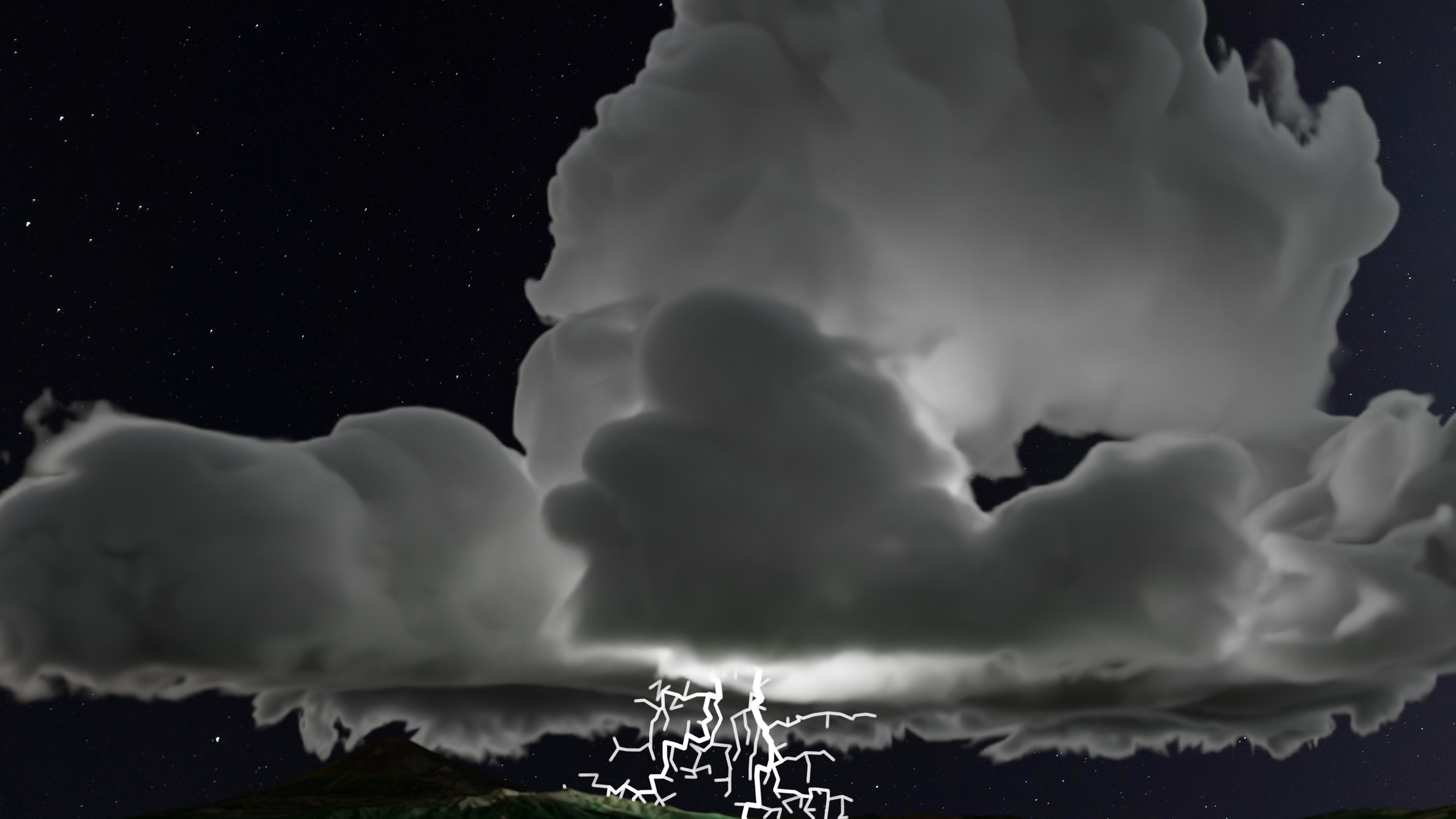
We simulate four common types of thunderstorms that occur within a mesoscale convective system (MCS), capturing their distinctive characteristics and dynamic behaviors:
-
•
Single Cell: Single cell thunderstorms, often referred to as “popcorn” convection, are small, isolated storms characterized by their brief lifespan, typically lasting less than an hour. These storms are visually compact with a single updraft and downdraft cycle, forming as isolated towering cumulus clouds.
-
•
Multicell: Multicell thunderstorms consist of clusters of individual convective cells, each at varying stages of development. They appear as a dynamic structure where new cells continuously form along the gust front, sustaining the system for several hours.
-
•
Squall Line: A squall line is a linear arrangement of thunderstorms, visually identifiable by a long and narrow band of cumulonimbus clouds. These storms can extend hundreds of miles in length but are typically narrow, often around 10-20 miles wide.
-
•
Supercell: The supercell is the most visually striking and organized thunderstorm type, dominated by a large, rotating updraft known as a mesocyclone. These storms feature massive, tilted, and rotating cloud structures, often rising up to 50,000 feet. The mesocyclone can span up to 10 miles in diameter and persists for hours.
These simulated variations allow us to explore the diverse behaviors and impacts of thunderstorms within an MCS. The visual comparison of these thunderstorm types is presented in Figure 6, highlighting their structural differences and unique features.
6.2. Severe Weather Phenomena
To explore the impact of thunderstorms in real-world scenarios, we reference severe weather events in geographically diverse locations. These events illustrate the variability and intensity of thunderstorms in different environments:
-
•
Biscayne National Park, Florida (25.3692, -80.243): On March 13, 1993, a tropical storm occurred in this region during the spring, bringing heavy rainfall and strong winds.
-
•
Chiricahua Mountains, New Mexico (35.7943, -106.443): On July 14, 1989, a severe thunderstorm swept through this mountainous area during the summer, producing heavy rain, hail, and strong winds.
-
•
Fuji-Hakone-Izu National Park, Japan (37.745, -119.54): On January 10, 2011, a sudden winter ;p‘thunderstorm formed in this region, resulting in brief but intense snowfall.
-
•
Monterey Bay, California (36.6197, -121.906): On December 2, 2012, an atmospheric river brought heavy rainfall and thunderstorms along the California coast, accompanied by strong gusty winds.
These events serve as the basis for our simulations, showcasing the capability of our model to replicate the diverse and complex phenomena associated with severe weather. The corresponding visualizations are presented in Figure 7.
7. VALIDATION
We adopt the evaluation methods outlined in (Shen et al., 2020) and (Cesana et al., 2019), utilizing altitude-based quantitative data to analyze cloud behavior across different atmospheric layers. The results are presented in Figure 8, which illustrates the relationship between cloud fraction and storm height. Notably, the maximum cloud fraction corresponds to the storm’s peak altitude, consistent with the classical vertical distribution of cumulonimbus clouds in meteorology.
For further validation, we specifically selected four regions frequently studied in thunderstorm meteorology (Uman, 2001; Harris and Carvalho, 2018). Following the methodology from (Herrera et al., 2021), we examine the temporal evolution of the thunderstorm described in section 6.2. The evolution of cloud coverage is compared with real-world weather data from public sources, showing dynamic changes in the distribution of cloud cover. This comparison helps assess the accuracy of the model in capturing cloud coverage patterns observed in nature.we present the maximum storm development height along with the corresponding cloud fraction, providing a detailed overview of the storm’s vertical structure. This information is used to validate the model’s ability to simulate the typical altitude and distribution of clouds during storm development.
In line with the evaluation method in (Formenton et al., 2013), we analyze the evolution of lightning flash rates to capture the electrical activity of thunderstorms. The flash rate increases as the storm develops and gradually declines to zero as the storm dissipates. This trend reflects the typical lifecycle of a thunderstorm and its charge dynamics. Additionally, the frequency of lightning occurrences is examined in relation to altitude.
Figure 9 provides a comparison across Florida, New Mexico, Japan, and California, illustrating the model’s ability to capture a wide range of climatic behaviors and atmospheric dynamics, and confirming its consistency with observed storm structures and lightning patterns.
8. CONCLUSION AND FUTURE WORK
We have developed a comprehensive framework for simulating atmospheric phenomena during thunderstorms, focusing on thundercloud development, dissipation, and lightning generation through cloud electrification processes. This framework integrates a Grabowski-style extended warm cloud microphysics scheme with hydrometeor electrification processes to ensure the consistent coupling of cloud formation and lightning dynamics. The model simulates key atmospheric quantities, including microphysical properties such as vapor, cloud water, ice, and precipitated rain and snow, as well as electrodynamic properties like static charge distribution and lightning flashes. Our framework reproduces various thundercloud types, including single-cell, multicell, squall line, supercell, and atmospheric river formations, and simulates lightning dynamics using the Dielectric Breakdown Model (DBM), capturing both CG and IC lightning. Validation against real-world weather data demonstrates the model’s accuracy in simulating cloud structure, temperature evolution, cloud coverage, relative humidity, and lightning flash rates, with results benchmarked against national weather services and observed lightning activity.
Future work will focus on expanding the framework to incorporate advanced atmospheric concepts and support a broader range of thunderstorm and lightning phenomena. Enhancements to thunderstorm microphysics, such as more detailed electrification processes and turbulence modeling, will improve the realism of lightning generation. The framework will also be extended to simulate additional thunderstorm types, including Mesoscale Convective Complex (MCC), Mesoscale Convective Vortex (MCV), and derechos, broadening its coverage of mesoscale systems. Furthermore, new lightning types such as anvil crawlers, bolts from the blue, and sheet lightning will be introduced, requiring refined electric field and branching models. Finally, scalability and real-time performance will be improved by leveraging advanced numerical techniques and hardware optimizations, enabling more detailed and efficient simulations.
References
- (1)
- Amador Herrera et al. (2024) Jorge Alejandro Amador Herrera, Jonathan Klein, Daoming Liu, Wojtek Pałubicki, Sören Pirk, and Dominik L Michels. 2024. Cyclogenesis: Simulating Hurricanes and Tornadoes. ACM Transactions on Graphics (TOG) 43, 4 (2024), 1–16.
- Anderson (1990) John David Anderson. 1990. Modern compressible flow: with historical perspective. (No Title) (1990).
- Atmosphere (1975) Standard Atmosphere. 1975. International organization for standardization. ISO 2533 (1975), 1975.
- Barthe and Pinty (2007) Christelle Barthe and Jean-Pierre Pinty. 2007. Simulation of a supercellular storm using a three-dimensional mesoscale model with an explicit lightning flash scheme. Journal of Geophysical Research: Atmospheres 112, D6 (2007).
- Cesana et al. (2019) Grégory Cesana, Anthony D Del Genio, and Hélène Chepfer. 2019. The cumulus and stratocumulus CloudSat-CALIPSO dataset (CASCCAD). Earth System Science Data 11, 4 (2019), 1745–1764.
- Dudhia (1989) Jimy Dudhia. 1989. Numerical study of convection observed during the winter monsoon experiment using a mesoscale two-dimensional model. Journal of Atmospheric Sciences 46, 20 (1989), 3077–3107.
- Ferreira Barbosa et al. (2015) Charles Welton Ferreira Barbosa, Yoshinori Dobashi, and Tsuyoshi Yamamoto. 2015. Adaptive cloud simulation using position based fluids. Computer Animation and Virtual Worlds 26, 3-4 (2015), 367–375.
- Formenton et al. (2013) M Formenton, G Panegrossi, D Casella, S Dietrich, A Mugnai, P Sanò, F Di Paola, H-D Betz, C Price, and Yoav Yair. 2013. Using a cloud electrification model to study relationships between lightning activity and cloud microphysical structure. Natural Hazards and Earth System Sciences 13, 4 (2013), 1085–1104.
- Garcia-Dorado et al. (2017) Ignacio Garcia-Dorado, Daniel G Aliaga, Saiprasanth Bhalachandran, Paul Schmid, and Dev Niyogi. 2017. Fast weather simulation for inverse procedural design of 3d urban models. ACM Transactions on Graphics (TOG) 36, 2 (2017), 1–19.
- Goswami and Neyret (2017) Prashant Goswami and Fabrice Neyret. 2017. Real-time landscape-size convective clouds simulation and rendering. In VRIPHYS 2017-13th Workshop on Virtual Reality Interaction and Physical Simulation.
- Grabowski (1998) Wojciech W Grabowski. 1998. Toward cloud resolving modeling of large-scale tropical circulations: A simple cloud microphysics parameterization. Journal of the Atmospheric Sciences 55, 21 (1998), 3283–3298.
- Hädrich et al. (2020) Torsten Hädrich, Miłosz Makowski, Wojtek Pałubicki, Daniel T Banuti, Sören Pirk, and Dominik L Michels. 2020. Stormscapes: Simulating cloud dynamics in the now. ACM Transactions on Graphics (TOG) 39, 6 (2020), 1–16.
- Harris and Carvalho (2018) Sarah M Harris and Leila MV Carvalho. 2018. Characteristics of southern California atmospheric rivers. Theoretical and applied climatology 132 (2018), 965–981.
- Herrera et al. (2021) Jorge Alejandro Amador Herrera, Torsten Hädrich, Wojtek Pałubicki, Daniel T Banuti, Sören Pirk, and Dominik L Michels. 2021. Weatherscapes: Nowcasting heat transfer and water continuity. ACM Transactions on Graphics (TOG) 40, 6 (2021), 1–19.
- Houze Jr (2014) Robert A Houze Jr. 2014. Cloud dynamics. Academic press.
- Kessler (1969) Edwin Kessler. 1969. On the distribution and continuity of water substance in atmospheric circulations. In On the distribution and continuity of water substance in atmospheric circulations. Springer, 1–84.
- Kessler (1995) Edwin Kessler. 1995. On the continuity and distribution of water substance in atmospheric circulations. Atmospheric research 38, 1-4 (1995), 109–145.
- Kim and Lin (2007) Theodore Kim and Ming C Lin. 2007. Fast animation of lightning using an adaptive mesh. IEEE Transactions on Visualization and Computer Graphics 13, 2 (2007), 390–402.
- Lastic et al. (2022) Maud Lastic, Damien Rohmer, Guillaume Cordonnier, Claude Jaupart, Fabrice Neyret, and Marie-Paule Cani. 2022. Interactive simulation of plume and pyroclastic volcanic ejections. Proceedings of the ACM on Computer Graphics and Interactive Techniques 5, 1 (2022), 1–15.
- Latham and Miller (1965) J Latham and AH Miller. 1965. The role of ice specimen geometry and impact velocity in the Reynolds-Brook theory of thunderstorm electrification. Journal of Atmospheric Sciences 22, 5 (1965), 505–508.
- Lin et al. (1983) Yuh-Lang Lin, Richard D Farley, and Harold D Orville. 1983. Bulk parameterization of the snow field in a cloud model. Journal of Applied Meteorology and climatology 22, 6 (1983), 1065–1092.
- Ma et al. (1998) Zhaofeng Ma, CL Croskey, and LC Hale. 1998. The electrodynamic responses of the atmosphere and ionosphere to the lightning discharge. Journal of atmospheric and solar-terrestrial physics 60, 7-9 (1998), 845–861.
- Mansell et al. (2002) Edward R Mansell, Donald R MacGorman, Conrad L Ziegler, and Jerry M Straka. 2002. Simulated three-dimensional branched lightning in a numerical thunderstorm model. Journal of Geophysical Research: Atmospheres 107, D9 (2002), ACL–2.
- Mansell et al. (2010) Edward R Mansell, Conrad L Ziegler, and Eric C Bruning. 2010. Simulated electrification of a small thunderstorm with two-moment bulk microphysics. Journal of the Atmospheric Sciences 67, 1 (2010), 171–194.
- Marshall et al. (1995) Thomas C Marshall, Michael P McCarthy, and W David Rust. 1995. Electric field magnitudes and lightning initiation in thunderstorms. Journal of Geophysical Research: Atmospheres 100, D4 (1995), 7097–7103.
- Miyazaki et al. (2002) Ryo Miyazaki, Yoshinori Dobashi, and Tomoyuki Nishita. 2002. Simulation of Cumuliform Clouds Based on Computational Fluid Dynamics.. In Eurographics (Short Presentations).
- Morrison et al. (2015) Hugh Morrison, Jason A Milbrandt, George H Bryan, Kyoko Ikeda, Sarah A Tessendorf, and Gregory Thompson. 2015. Parameterization of cloud microphysics based on the prediction of bulk ice particle properties. Part II: Case study comparisons with observations and other schemes. Journal of the Atmospheric Sciences 72, 1 (2015), 312–339.
- Niemeyer et al. (1984) Lucian Niemeyer, Luciano Pietronero, and Hans J Wiesmann. 1984. Fractal dimension of dielectric breakdown. Physical Review Letters 52, 12 (1984), 1033.
- Pretorius et al. (2024) Pieter C Pretorius, James Gain, Maud Lastic, Guillaume Cordonnier, Jiong Chen, Damien Rohmer, and M-P Cani. 2024. Volcanic Skies: coupling explosive eruptions with atmospheric simulation to create consistent skyscapes. In Computer Graphics Forum, Vol. 43. Wiley Online Library, e15034.
- Rabbani et al. (2022) Amir Hossein Rabbani, Jean-Philippe Guertin, Damien Rioux-Lavoie, Arnaud Schoentgen, Kaitai Tong, Alexandre Sirois-Vigneux, and Derek Nowrouzezahrai. 2022. Compact Poisson Filters for Fast Fluid Simulation. In ACM SIGGRAPH 2022 Conference Proceedings. 1–9.
- Reed and Wyvill (1994) Todd Reed and Brian Wyvill. 1994. Visual simulation of lightning. In Proceedings of the 21st annual conference on Computer graphics and interactive techniques. 359–364.
- Shen et al. (2020) Zhaoyi Shen, Kyle G Pressel, Zhihong Tan, and Tapio Schneider. 2020. Statistically steady state large-eddy simulations forced by an idealized GCM: 1. Forcing framework and simulation characteristics. Journal of Advances in Modeling Earth Systems 12, 2 (2020), e2019MS001814.
- Solomon et al. (2005) R Solomon, CM Medaglia, C Adamo, S Dietrich, A Mugnai, and Ugo Biader Ceipidor. 2005. An explicit microphysics thunderstorm model. International Journal of Modelling and Simulation 25, 2 (2005), 112–118.
- Stam (1999) Jos Stam. 1999. Stable fluids. In Proceedings of the 26th Annual Conference on Computer Graphics and Interactive Techniques (SIGGRAPH ’99). ACM Press/Addison-Wesley Publishing Co., USA, 121–128. https://doi.org/10.1145/311535.311548
- Uman (2001) Martin A Uman. 2001. The lightning discharge. Courier Corporation.
- Vimont et al. (2020) Ulysse Vimont, James Gain, Maud Lastic, Guillaume Cordonnier, Babatunde Abiodun, and Marie-Paule Cani. 2020. Interactive Meso-scale Simulation of Skyscapes. In Computer Graphics Forum, Vol. 39. Wiley Online Library, 585–596.
- Webanck et al. (2018) Antoine Webanck, Yann Cortial, Eric Guérin, and Eric Galin. 2018. Procedural cloudscapes. In Computer Graphics Forum, Vol. 37. Wiley Online Library, 431–442.
- Wendt (2008) John F Wendt. 2008. Computational fluid dynamics: an introduction. Springer Science & Business Media.
- Wu et al. (2023) Kenan Wu, Tianwen Wei, Jinlong Yuan, Haiyun Xia, Xin Huang, Gaopeng Lu, Yunpeng Zhang, Feifan Liu, Baoyou Zhu, and Weidong Ding. 2023. Thundercloud structures detected and analyzed based on coherent Doppler wind lidar. Atmospheric Measurement Techniques Discussions 2023 (2023), 1–22.
- Yau and Rogers (1996) Man Kong Yau and Roddy Rhodes Rogers. 1996. A short course in cloud physics. Elsevier.
- Yun et al. (2017) Jeongsu Yun, Myungbae Son, Byungyoon Choi, Theodore Kim, and Sung-Eui Yoon. 2017. Physically inspired, interactive lightning generation. Computer Animation and Virtual Worlds 28, 3-4 (2017), e1760.
- Zhang et al. (2020) Zili Zhang, Yunfei Li, Bailin Yang, Frederick WB Li, and Xiaohui Liang. 2020. Target-driven cloud evolution using position-based fluids. Computer Animation and Virtual Worlds 31, 6 (2020), e1937.