Throughput of Freeway Networks under Ramp Metering Subject to Vehicle Safety Constraints
Abstract
Ramp metering is one of the most effective tools to combat traffic congestion. In this paper, we present a ramp metering policy for a network of freeways with arbitrary number of on- and off-ramps, merge, and diverge junctions. The proposed policy is designed at the microscopic level and takes into account vehicle following safety constraints. In addition, each on-ramp operates in cycles during which it releases vehicles as long as the number of releases does not exceed its queue size at the start of the cycle. Moreover, each on-ramp dynamically adjusts its release rate based on the traffic condition. To evaluate the performance of the policy, we analyze its throughput, which is characterized by the set of arrival rates for which the queue sizes at all on-ramps remain bounded in expectation. We show that the proposed policy is able to maximize the throughput if the merging speed at all the on-ramps is equal to the free flow speed and the network has no merge junction. We provide simulations to illustrate the performance of our policy and compare it with a well-known policy from the literature.
I Introduction
Ramp metering, which controls the inflow of traffic to a freeway, is one of the most efficient tools to combat traffic congestion. In this paper, we propose a microscopic (vehicle)-level ramp metering policy for freeway networks with arbitrary number of on- and off-ramps, merge and diverge junctions. Our approach builds up on our previous work [1], where we considered a single freeway with no merge or diverge junctions.
Ramp metering policies are commonly designed using macroscopic traffic flow models, which use spatio-temporal averaging of vehicle interactions to model the traffic. Many ramp metering policies have been proposed in the literature using this approach [2, 3]. These policies are either: (i) fixed-time [4], where no real-time traffic measurement is used, or (ii) local traffic-responsive [5], where on-ramps use only local measurements, or (iii) coordinated traffic-responsive [6, 7, 8], where on-ramps also use measurements from other parts of the network. In spite of its generality, the macroscopic-level approach is not suitable in the context of Connected and Automated Vehicles (CAVs) as it does not capture some of their capabilities, such as the ability to dissipate traffic disturbance and provide accurate measurements of traffic through Vehicle-to-Vehicle (V2V) and Vehicle-to-Infrastructure (V2I) communication systems [9, 10, 11]. Additionally, macroscopic-level ramp metering policies do not account for vehicle following safety constraints. As a consequence, the vehicles may find themselves in unsafe situations near an on-ramp, which can trigger congestion or even an accident. While adding safety filters on top of the ramp metering policy is a potential solution, it may adversely affect other performance criteria such as the total travel time [1].
A more systematic approach is to explicitly include vehicle safety, connectivity, and automation protocols in the ramp metering design by considering the vehicles at the microscopic level. Somewhat surprisingly, the literature on the microscopic-level ramp metering design is sparse and only limited to isolated on-ramps [12, 13]. Relatively little attention has been given to analyzing the overall performance of a freeway network. For example, are certain system-level performance metrics such as throughput optimized? To bridge this gap and expand our previous work for a single freeway [1], we consider a network of freeways to design and analyze a microscopic ramp metering policy that can maximize the throughput.
The freeway network is modeled as a directed acyclic graph, with arbitrary number of on- and off-ramps, merge, and diverge junctions. Vehicles arrive from outside the network to the on-ramps and join the on-ramp queues. The on-ramp arrivals are sampled from i.i.d Bernoulli processes that are independent across different on-ramps, and the vehicle routes are sampled independently from a routing matrix. Once released from an on-ramp, each vehicle follows standard safety and speed rules until it reaches its destination off-ramp. Vehicles in the network have the same acceleration and braking capabilities, and are equipped with V2V and V2I communication systems. We leverage these connectivity capabilities to design a coordinated traffic-responsive ramp metering policy. The proposed policy operates under vehicle following safety constraints, where new vehicles are released only if there is enough gap on the mainline. Additionally, the on-ramps operate under synchronous cycles during which each on-ramp does not release more vehicles than its queue size at the start of the cycle. Moreover, an on-ramp’s release rate is adjusted during a cycle according to the traffic condition in the network.
We evaluate the performance of a policy in terms of its throughput, which is characterized by the set of arrival rates under which the queue sizes at every on-ramp remain bounded in expectation. We show that the proposed policy is able to maximize the throughput when the merging speed at all the on-ramps equals the free flow speed and the network has no merge junction, e.g., a single freeway.
The remainder of the paper is organized as follows: in Section II, we describe the network structure, the vehicles behavior in the network, the demand model, and the performance metric. We provide our ramp metering policy and its performance analysis in Section III. We provide simulation results in Section IV, and conclude the paper in Section V.
We collect key notations to be used throughout the paper. Let and respectively denote the set of positive integers, and non-negative integers. For , denotes the set . For a set , denotes its cardinality.
II Problem Formulation
II-A Network Topology
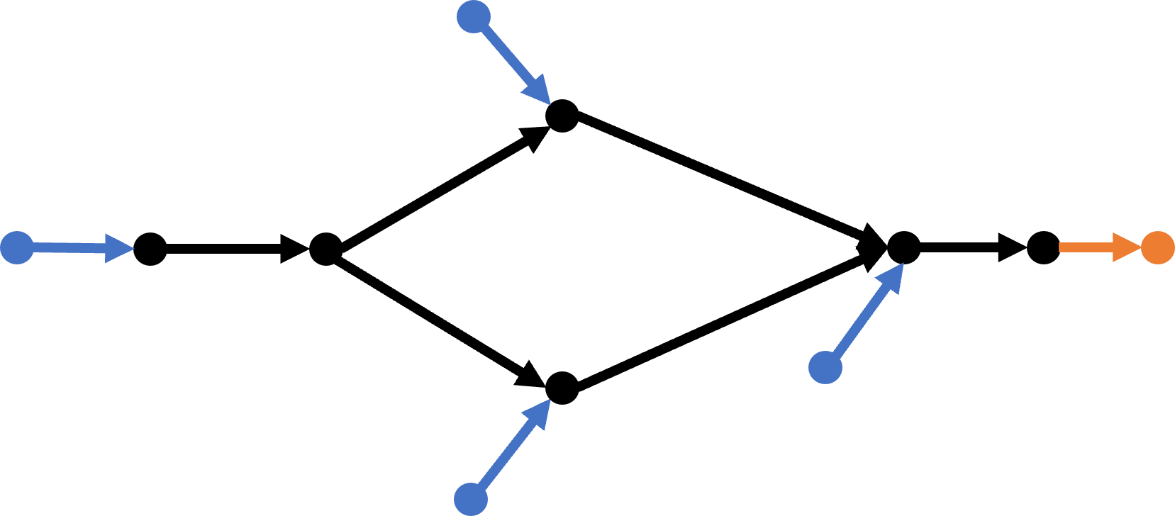
The network is modeled as a directed acyclic graph. The nodes represent either junctions (merge or diverge), or sources/sinks; the edges represent either single-lane freeway segments that connect two junctions, or on- and off-ramps that connect sources to merge nodes and diverge nodes to sinks, respectively; see Figure 1. We refer to any subset of the freeway segments as the mainline. For simplicity, we assume that each source has exactly one outgoing on-ramp, and each sink has exactly one incoming off-ramp. We distinguish between two types of merge node: on-ramp nodes, which have at least one incoming on-ramp, and regular merge nodes (or simply merge nodes), which have no incoming on-ramp. Similarly, we distinguish between an off-ramp node and a diverge node. We denote the set of on-ramp nodes by . For simplicity, we assume that each on-ramp node has exactly one incoming on-ramp edge. Thus, also specifies the set of on-ramp edges. For on-ramp , we let be the set of its successor on-ramps, i.e., the set of all on-ramps that are immediately downstream of on-ramp . An element of is denoted by . Similarly, we let be the set of its predecessor on-ramps. We say that two edges are adjacent if the head of one edge is the tail of the other edge. A route is a sequence of adjacent edges, with the first edge being an on-ramp and the last edge being an off-ramp. The collection of all routes is denoted by .
Vehicles arrive to on-ramps according to some exogenous stochastic process and join the on-ramp queues. For any on-ramp, we assume a point queue model with unlimited capacity. We also assume that vehicles that reach their destination off-ramp node, immediately leave the network without creating any obstruction. Once a vehicles is released from an on-ramp into the mainline, it follows standard speed and safety rules, which will be explained in the following section.
II-B Vehicle-Level Objectives
Vehicles have the same length , the same acceleration and braking capabilities, and are equipped with V2V and V2I communication systems. The exact information communicated by a vehicle will be specified in Section III, where we introduce our ramp metering policy. We use the term ego vehicle to refer to a specific vehicle under consideration, and denote it by . Consider a vehicle following scenario and let (resp. ) be the speed of the ego vehicle (resp. its leading vehicle), and be the safety distance between the two vehicles required to avoid collision. We assume that satisfies , which is calculated based on an emergency stopping scenario with details given in [14]. Here, is a safe time headway constant, is an additional constant gap, and is the minimum possible deceleration of the leading vehicle. We consider two general modes of operation for each vehicle: the speed tracking mode and the safety mode. The main objective in the speed tracking mode is to adjust and maintain the speed to the free flow speed when the ego vehicle is far from any leading vehicle; the main objective in the safety mode is to avoid rear-end collision once the ego vehicle gets close to the leading vehicle.
We assume that vehicles obey the following rules:
-
(VC1)
The ego vehicle maintains the constant speed if:
-
(a)
it is at a safe distance with respect to its leading vehicle 111At a diverge node, the leading vehicle is uniquely determined by the ego vehicle’s route choice., i.e., , where is the distance between the two vehicles. Note that if its leading vehicle is also at the constant speed , then . This distance is equivalent to a time headway of at least between the front bumpers of the two vehicles.
-
(b)
it is near a merge node and predicts to be at a safe distance with respect to its leading vehicle after reaching the merging node, i.e., , where is the time the ego vehicle predicts to reach the merge node, is the predicted distance between the two vehicles, and is the predicted speed. Each vehicle uses the following speed prediction rule to calculate its predicted time of merging, position, and speed: if in the speed tracking mode, it assumes that it remains in this mode in the future; if in the safety mode, it assumes a constant speed trajectory. These information are then communicated among all vehicles near a merge node via V2V communication.
-
(a)
-
(VC2)
there exists such that for any initial condition, vehicles reach the free flow equilibrium after at most time if no other vehicle is released from the on-ramps. The free flow equilibrium refers to a state where each vehicle is moving at the constant speed and will maintain this speed in the future if no additional vehicle is released from the on-ramps.
Remark 1.
Due to lack of space, we assume that the ego vehicle immediately joins the mainline after being released. In other words, we ignore the vehicle dynamics between release from an on-ramp and joining the mainline. We also assume the speed at which the ego vehicle joins the mainline, i.e., the merging speed, is . The general case where these assumptions are relaxed can be treated similar to [1]. We should emphasize, however, that the merging speed assumption can affect the performance of a ramp metering policy; see Remark 3.
In order to have a complete description of the network, we also need to specify the demand at the microscopic level. We will do this in the next section.
II-C Demand Model
For convenience in the analysis, we adopt a discrete time setting with time steps of size , where is the minimum safe time headway at the free flow speed defined in Section II-B. Let vehicles arrive to on-ramp according to an i.i.d. Bernoulli process with parameter . The arrival processes are assumed to be independent across different on-ramps. That is, at any given time step, the probability that a vehicle arrives at the -th on-ramp is independent of everything else. We let . A vehicle arriving to on-ramp , chooses to take route with probability independent of everything else. Naturally, for every on-ramp , , and for any that is not compatible with the network topology. We assume that the vehicles do not change their route choice while in the network. We stack the routing probabilities in a routing matrix . Let be the average induced load on on-ramp , where the notation means that on-ramp ’s node is on route . This is the average number of arrivals in the network that wants to cross on-ramp ’s node in order to reach their destination. The performance of a ramp metering policy is quantified in terms of the maximum demand it can handle. We will formalize this in the next section.
II-D Ramp Metering and Performance Metric
To conveniently track vehicle locations in discrete time, we introduce the notion of slot. A slot is associated with a particular point on the mainline at a particular time. Consider the maximum number of distinct slots that can be placed on a freeway segment, such that the distance between adjacent slots is , i.e., the minimum safety distance at the free flow speed as per (VC1) plus the vehicle length. Consider a configuration of these slots at . At the end of each time step , each slot replaces the next slot with the last slot replacing the first slot of that segment. Without loss of generality, we let the location of the first and last slots of each segment coincide with the tail and head of that segment at the end of each time step. Thus, if the ego vehicle is released from an on-ramp at the end of a given time step, its location coincides with a slot.
For , let be the set of the route choices of the vehicles waiting at on-ramp , arranged in the order of their arrival, at time . We use to denote the queue size at on-ramp at time . Let be the vector of queue sizes at all the on-ramps at time . A ramp metering policy is a function , where if a vehicle is released from on-ramp at time , and otherwise. The key metric we use to evaluate the performance of a ramp metering policy is its throughput, which is defined as follows: for a given ramp metering policy and routing matrix , let be the set of ’s for which for all . We say that the network is under-saturated if ; otherwise, it is called saturated. The throughput is the boundary of the set . We are interested in finding a ramp metering policy such that for every and any other policy , we have . We say such a policy maximizes the throughput.
III Main Results
III-A Dynamic Release Rate Policy with Rate Allocation
In this section we present and analyze our ramp metering policy. The policy presented is coordinated, in the sense that each on-ramp may require information from other parts of the network in addition to the information obtained from its vicinity. However, it does not require any information about the demand or the route choice of the vehicles, i.e., it is reactive [15]. The policy operates under synchronous cycles of fixed length during which each on-ramp does not release more vehicles than its queue size at the beginning of the cycle. The synchronization of cycles is done once offline. This policy allocates a fixed maximum release rate to each on-ramp. In addition, it imposes dynamic minimum time gap criterion between release of successive vehicles from the same on-ramp. Changing the time gap between release of successive vehicles by an on-ramp is akin to changing its release rate. An inner approximation to the throughput of this policy is provided, and is then compared to an outer approximation.
Definition 1.
(Dynamic Release Rate policy with rate Allocation (DRRA)) The policy works in cycles of fixed length , where . At the beginning of the -th cycle at , each on-ramp allocates itself a “quota” equal to the queue size at that on-ramp at . At time during the -th cycle, on-ramp releases the ego vehicle if:
-
(M1)
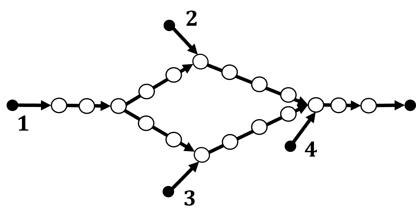
, where , , and , , are such that the release times at all the on-ramps are conflict-free, meaning that no two vehicles that move at the constant speed after being released can simultaneously reach a merging node; see Figure 2. The term is the maximum release rate allocated to on-ramp .
-
(M2)
the on-ramp has not reached its quota.
-
(M3)
the ego vehicle is at a safe distance with respect to its leading and following vehicles at the moment of release.
-
(M4)
at least time has passed since the release of the last vehicle from on-ramp .
Once an on-ramp reaches its quota, it does not release a vehicle during the rest of the cycle. The minimum time gap is piecewise constant, updated periodically at , as described in Algorithm 1. In Algorithm 1, is defined as follows: for the ego vehicle, let , where is the indicator function, and is the acceleration. The state of all the vehicles is collectively denoted as , where is the total number of vehicles on the mainline. We let . Moreover, for , let , where the sum is over all the vehicles in the time interval that predicted to violate the safety distance after reaching a merging node. We let . Roughly, measures the distance to the free flow equilibrium state at time .
Theorem 1.
For any initial condition, , design constants in Algorithm 1, and such that , , and the release times are conflict-free, the DRRA policy keeps the network under-saturated if for all .
Proof.
See Appendix B. ∎
V2I communication requirements: This policy uses information about (if ) and . After a finite time, the mainline vehicles only communicate to all the on-ramps at the end of each update period . The number of vehicles that constitute is no more than the total number of slots. Furthermore, at the end of each time step during a cycle, the vehicles near an on-ramp communicate their state to that on-ramp for the safety gap evaluation.
Remark 2.
A non-reactive version of the DRRA policy with better throughput: suppose that the first vehicle in every on-ramp’s queue also communicates its route choice to that on-ramp. Consider a version of the DRRA policy, where, in addition to the releasing times in (M1), on-ramp releases the ego vehicle at , , if the ego vehicle’s route contains no merge node. This policy is non-reactive since it uses the route choice of the vehicles, but gives a better throughput since more vehicles are released compared to the DRRA policy. We compare the performance of these two policies via simulations in Section IV.
Remark 3.
Recall from Section II-B that we made the simplifying assumption that the merging speed at all the on-ramps is . One can relax this assumption, but the throughput would suffer due to the larger safety distance required at the moment of merging. However, the main steps of the proof of Theorem 1 remain the same and a similar bound for the throughput can be obtained; see [1, Theorem 2].
III-B A Necessary Condition
We now provide a necessary condition for under-saturation, against which we benchmark the sufficient condition in Theorem 1. Let be the cumulative number of vehicles that has crossed point on the mainline up to time , , under the ramp-metering policy . Then, the crossing rate at point is defined as and the “long-run” crossing rate is . Recall the definition of for on-ramp ’s node. We can extend this definition to every node in the network that is not a source or sink. Let , where is any node that is not a source or sink.
Theorem 2.
Suppose that the long-run crossing rate is no more than one vehicle per seconds for at least one point on each freeway segment. If the network is under-saturated under the policy , then .
Proof.
The proof is similar to [1, Theorem 4]. ∎
Remark 4.
Remark 5.
Consider a network with no merge node, and note that for any node that is not a source or sink, we have for some . For such a network, one can set for all in the DRRA policy. The sufficient condition of Theorem 1 then becomes . Combining with Theorem 2, it follows for any routing matrix and any other ramp metering policy that , except, maybe at the boundary of . Since the boundary of has zero volume (measure), we can conclude that the DRRA policy maximizes the throughput for all practical purposes.
IV Simulations


We simulate the DRRA policy and compare its performance with its non-reactive version introduced in Remark 2 and a well-known policy from the literature. All the simulations were performed in MATLAB. We use the following setup in all the simulations: let , , , and . The initial queue size at all the on-ramps is set to zero, and vehicles arrive at the on-ramps according to i.i.d Bernoulli processes with the same rate .
IV-A Total Travel Time
In this section, we compare the total travel time under the DRRA policy and ALINEA [5], which is a macroscopic ramp metering policy. We also add the safety filter (M3) on top of ALINEA, and use the name Safe-ALINEA to refer to the resulting policy. An on-ramp’s outflow in the ALINEA policy is determined according to the following equation:
Here, is the on-ramp’s outflow, is a positive design constant, is the occupancy of the mainline downstream of the on-ramp, and is the desired occupancy. We use time steps of size , [5], and corresponding to the capacity flow. For the DRRA policy, we use the following parameters: , , , , , , and , . The network is a ring road with perimeter and on- and off-ramps. The on-ramps are located symmetrically at locations , , and ; the off-ramps are also located symmetrically upstream of each on-ramp. We consider a congested initial condition where the initial number of vehicles on the mainline is ; each vehicle is at the constant speed of , and is at the distance from its leading vehicle. The details of the vehicle following behavior is given in [1]. We also let and
where columns specify the off-ramps.
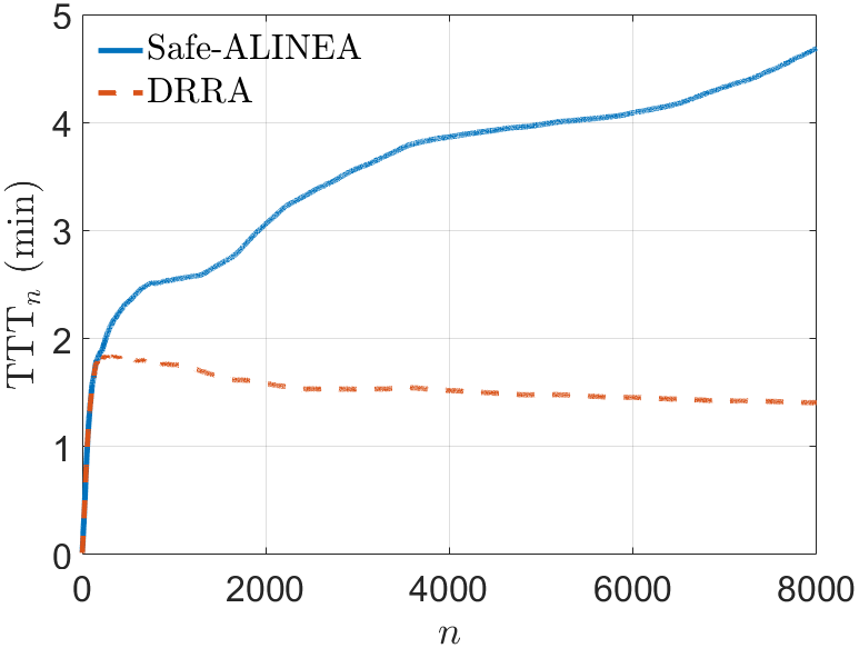
We evaluate the average Total Travel Time (TTTn), which is computed by averaging the total travel time of the first vehicles that complete their trips. The total travel time of a vehicle equals its waiting time in an on-ramp queue plus the time it spends on the freeway to reach its destination. Figure 3 shows the simulation result. From the figure, we can see that the DRRA policy provides significant improvement in the TTTn compared to the Safe-ALINEA policy. In fact, the network becomes saturated under the Safe-ALINEA policy, which implies that the TTTn will grow steadily with .
IV-B Acyclic Network with Merge Junction
The second network is a symmetric three-legged merge junction; see Figure 4(a). The total length of freeway segments on each leg is . on-ramps and are located at the beginning, while on-ramp is located in the middle of their corresponding legs. Similarly, off-ramps and are in the middle, while off-ramp is at the end of their corresponding legs. The mainline is initially empty and
The on-ramps use the DRRA policy with and other parameters chosen similar to Section IV-A. In addition, the release times of on-ramps and are set to and , respectively, while for on-ramp , (thus, , , , and ). For the given routing matrix, the inner and outer estimates of the under-saturation region given by Theorems 1 and 2 are and , respectively. From simulations, the under-saturation regions of the DRRA policy and its non-reactive version are estimated to be and , respectively. This suggest that there is a gap between the inner and outer estimates of the under-saturation region in the DRRA policy, but not in its non-reactive version.
IV-C Cyclic Network with Merge Juction
The third network is constructed by making the second network cyclic; see Figure 4(b). The length of the additional segment in this network is . The mainline is initially empty and
The on-ramps again use the DRRA policy with the same parameters as in the previous section. The inner and outer estimates of the under-saturation region are and , respectively. From simulations, the under-saturation regions of the DRRA policy and its non-reactive version are estimated to be and , respectively. Therefore, Theorem 1 holds for this cyclic network. Based on the simulation results and the results in [1] given for a ring road network, we conjecture that Theorem 1 holds for general cyclic networks.
V Conclusion and Future Work
In this paper, we provided a microscopic ramp metering policy for freeway networks with arbitrary number of on- and off-ramps, merge, and diverge junctions. We analyzed the throughput of our policy for acyclic networks, and showed via simulations that it achieves a similar throughput for cyclic networks. We plan to confirm this observation analytically in the future. Moreover, we plan to extend our analysis to policies with tighter estimates of the throughput.
References
- [1] M. Pooladsanj, K. Savla, and P. A. Ioannou, “Saturation region of freeway networks under safe microscopic ramp metering,” arXiv preprint arXiv:2207.02360, 2022.
- [2] M. Papageorgiou and A. Kotsialos, “Freeway ramp metering: An overview,” IEEE transactions on intelligent transportation systems, vol. 3, no. 4, pp. 271–281, 2002.
- [3] M. Papageorgiou, C. Diakaki, V. Dinopoulou, A. Kotsialos, and Y. Wang, “Review of road traffic control strategies,” Proceedings of the IEEE, vol. 91, no. 12, pp. 2043–2067, 2003.
- [4] J. A. Wattleworth, “Peak-period analysis and control of a freeway system,” tech. rep., Texas Transportation Institute, 1965.
- [5] M. Papageorgiou, H. Hadj-Salem, J.-M. Blosseville, et al., “Alinea: A local feedback control law for on-ramp metering,”
- [6] M. Papageorgiou, J.-M. Blosseville, and H. Haj-Salem, “Modelling and real-time control of traffic flow on the southern part of boulevard périphérique in paris: Part ii: Coordinated on-ramp metering,” Transportation Research Part A: General, vol. 24, no. 5, pp. 361–370, 1990.
- [7] I. Papamichail, A. Kotsialos, I. Margonis, and M. Papageorgiou, “Coordinated ramp metering for freeway networks–a model-predictive hierarchical control approach,” Transportation Research Part C: Emerging Technologies, vol. 18, no. 3, pp. 311–331, 2010.
- [8] G. Gomes and R. Horowitz, “Optimal freeway ramp metering using the asymmetric cell transmission model,” Transportation Research Part C: Emerging Technologies, vol. 14, no. 4, pp. 244–262, 2006.
- [9] R. E. Stern, S. Cui, M. L. Delle Monache, R. Bhadani, M. Bunting, M. Churchill, N. Hamilton, H. Pohlmann, F. Wu, B. Piccoli, et al., “Dissipation of stop-and-go waves via control of autonomous vehicles: Field experiments,” Transportation Research Part C: Emerging Technologies, vol. 89, pp. 205–221, 2018.
- [10] M. Pooladsanj, K. Savla, and P. Ioannou, “Vehicle following over a closed ring road under safety constraint,” in 2020 IEEE Intelligent Vehicles Symposium (IV), pp. 413–418, IEEE.
- [11] M. Pooladsanj, K. Savla, and P. A. Ioannou, “Vehicle following on a ring road under safety constraints: Role of connectivity and coordination,” IEEE Transactions on Intelligent Vehicles, vol. 8, no. 1, pp. 628–638, 2022.
- [12] J. Rios-Torres and A. A. Malikopoulos, “Automated and cooperative vehicle merging at highway on-ramps,” IEEE Transactions on Intelligent Transportation Systems, vol. 18, no. 4, pp. 780–789, 2016.
- [13] J. Rios-Torres and A. A. Malikopoulos, “A survey on the coordination of connected and automated vehicles at intersections and merging at highway on-ramps,” IEEE Transactions on Intelligent Transportation Systems, vol. 18, pp. 1066–1077, May 2017.
- [14] P. Ioannou and C. Chien, “Autonomous intelligent cruise control,” IEEE Transactions On Vehicular Technology, vol. 42, no. 4, pp. 657–672, 1993.
- [15] I. Papamichail and M. Papageorgiou, “Traffic-responsive linked ramp-metering control,” IEEE Transactions on Intelligent Transportation Systems, vol. 9, no. 1, pp. 111–121, 2008.
- [16] S. P. Meyn and R. L. Tweedie, Markov chains and stochastic stability. Springer Science & Business Media, 2012.
- [17] G. B. Folland, Real analysis: modern techniques and their applications, vol. 40. John Wiley & Sons, 1999.
Appendix A Performance Analysis Tool
Consider an initial condition where the vehicles are in the free flow equilibrium, and the location of each vehicle coincides with a slot. Thus, their location coincide with a slot in the future. Thereafter, during each time step, the following sequence of events occurs: (i) the slots on each segment replace the next slot with the last slot replacing the first slot; the numbering of slots is reset with the new first slot numbered , and the rest numbered in an increasing order in the direction of the flow, (ii) vehicles that reach their destination off-ramp exit the network, (iii) if permitted by the ramp metering policy, a vehicle is released into a slot at the free flow speed. Since the initial location of all vehicles coincide with a slot and the released times are conflict-free, the location of the released vehicle will also coincide with a slot in the future.
For the aforementioned initial condition, we can cast the network dynamics as a discrete-time Markov chain, with time steps of size . Let be the set of the routes of the occupants of all the slots: if the vehicle occupying slot at time has to take route , and if slot is empty at time . Consider the following discrete-time Markov chain with the state , , where , and will be specified for the policy being analyzed. The transition probabilities are determined by the ramp metering policy being analyzed, but will not be specified explicitly for brevity. For the ramp metering policy considered in this paper, the state is reachable from all other states, and . Hence, the Markov chain is irreducible and aperiodic.
Appendix B Proof of Theorem 1
For any initial condition, we first show that there exists some such that for all , . This and (VC1) imply that every vehicle moves at the free flow speed for all . Hence, after a finite time after , , and the location of every vehicle coincides with a slot thereafter. We can then use the Markov chain setting from Appendix A.
Using an argument similar to [1], one can easily show that is uniformly bounded for all . To show after a finite time, we use a proof by contradiction. Suppose that for infinitely many . Since is uniformly bounded, there exists an infinite sequence such that for all . This implies that for all . Since is non-decreasing and , it follows that , which in turn implies that . Let be such that , where is an upper bound on the additional time required for all vehicles on the mainline to leave the network after reaching the free flow state, if no additional vehicle is released. Let . Note that for all , . Thus, each on-ramp releases at most one vehicle during the interval . Hence, there exists a time interval of length at least in during which no on-ramp releases a vehicle. Condition (VC2) then implies that all vehicles reach the free flow state after at most time, and leave the network after at most an additional time, at the end of which (say at time ), the network becomes empty. Thus, for all , , which is a contradiction to the assumption that for infinitely many .

We assume that the vehicles are initially in the free flow equilibrium state, and the location of each vehicle coincides with a slot at as in Appendix A. For the sake of readability, we present proofs of intermediate claims at the end. We adopt the Markov chain setting from Appendix A with as the Markov chain, where and is to be determined. For on-ramp , let be the degree of on-ramp representing the number of vehicles in the network at time that need to cross on-ramp ’s node in order to reach their destination. We recursively define the following collections of index sets:
and for ,
where each is treated as a multiset; see Figure 5. In words, , i.e., , is the set of all on-ramps that precede on-ramp ; if , then for any on-ramp that precedes on-ramp , either or all on-ramps that precede belong to ; and so on. Note that since the network is acyclic, the number of sets is finite for every . Let . Consider the candidate Lyapunov function defined as:
| (1) |
where is the range of values of in Appendix A, and .
Note that (1) implies . We show at the end of the proof that if is large enough, specifically if , where and , then
| (2) |
where satisfies the following: it is independent of , and there exists such that for all we have
| (3) |
The inequality (2) implies that
| (4) | ||||
By choosing and taking conditional expectation from both sides of (4) we obtain
Since for any , , we have . Hence, choosing gives
If is chosen such that for all ,
| (5) | ||||
then . Such a always exists because the term in (5) dominates for sufficiently large . We let be the minimum natural number that is divisible by .
Finally, if , then . Also, because the total number of arrivals at each time step does not exceed . Combining this with the previously considered case of , we get
where (a finite set). The result then follows from the well-known Foster-Lyapunov drift criterion [16, Theorem 14.0.1].
Proof of (2)
Consider on-ramp . If for every interval in , vehicles cross on-ramp , then
where is the total number of arrivals in the network during the time interval that want to cross on-ramp ’s node in order to reach their destination. If not, then there exist some time step in during which a valid slot that is empty crosses on-ramp ’s node. Let be the last time step at which this happens, i.e., . Hence,
| (6) | ||||
By the assumption of the theorem, i.e., for all , there exists such that for all ,
Thus, (6) can be rewritten as
| (7) | ||||
Furthermore, the queue size at on-ramp at time cannot exceed , i.e., . This is because, a valid slot that is empty crosses on-ramp at time step . Therefore, the quotas of on-ramp at time must be zero. This implies that only consists of vehicles arriving after the start of the most recent cycle before . Since the number of arrivals to on-ramp is no more than one per time step, it follows that . Hence, , where is the total number of slots between on-ramp and any on-ramp . Combining this with (7) gives
| (8) | ||||
Repeating the above steps for any on-ramp gives
where is defined similar to if at least one valid slot that is empty crosses on-ramp , and otherwise. This process can be repeated until we find a multiset of on-ramps, such that for each with multiplicity , either , or and , . Indeed, such a always exist since the network is acyclic. Let be a multiset containing all the on-ramps visited in this process (for example, if , then ). For simplicity of notation, we drop the superscript in with the understanding that could take different values for on-ramps with multiplicity greater than one. We also use to denote an on-ramp that succeeds on-ramp . By combining all the inequalities in this process we obtain
Note that if for some , then , which implies . Therefore, , where
| (9) | ||||
where we have dropped the dependence of on other parameters for brevity. Generally, if we start with any , we can repeat the above steps to obtain , where has the same form as (9), with defined similarly. Hence, (2) follows with
| (10) |
Note that for each , we may assume that there exists some for which . For if for all , then for all , which implies
| (11) |
where in the first inequality we have used the following fact: the total number of arrivals to the network is bounded by at each time step. Hence, for each , . Also, in the third inequality we have used the following fact: decreases by at most one during each time step. Therefore, . The inequality (11) implies that we can exclude from the maximum in (10). Thus, we may assume such with exists.
Proof of (3)
Given with the corresponding multiset , let for some . Hence, there exists a sequence of on-ramps with and such that for , . Therefore, . Consider the sequence , where the indices are allowed to depend on time . For a given , the term is independent of the other terms in the sequence, is bounded, and is (uniformly) bounded for all . As a result, is also bounded. From Kolmogorov’s strong law of large numbers [17, Theorem 10.12], we have, with probability ,
Hence, with probability one, there exists such that and for we have
This implies that, with probability one, for we have
Furthermore, for any other , with probability one, there exists such that implies , and if , then , since the total number of arrivals to the network is bounded by at each time step. Therefore, with probability one, for we have
| (12) | ||||
which in turn implies that, with probability one, . It follows that, with probability one, .
Finally,
| (13) |
where we have used in the first inequality using the fact that the total number of arrivals to the network is bounded by at each time step. Therefore, the sequences and are upper bounded by integrable functions. Fatou’s lemma [17] then implies
where is some constant. This in turn gives (3).