Threshold KNN-Shapley: A Linear-Time and Privacy-Friendly Approach to Data Valuation

The Shapley value (SV) [Sha53] is a classic concept from game theory to attribute the total gains generated by the coalition of all players. At a high level, it appraises each point based on the (weighted) average utility change caused by adding the point into different subsets of the training set. Formally, given a utility function $v(\cdot)$ and a training set $D$, the Shapley value of a data point $z\in D$ is defined as

For notation simplicity, when the context is clear, we omit the utility function and/or leave-one-out dataset, and write $\phi_{z}(D_{-z})$, $\phi_{z}(v)$ or $\phi_{z}$ depending on the specific dependency we want to stress.

The popularity of the Shapley value is attributable to the fact that it is the unique data value notion satisfying four axioms: Dummy player, Symmetry, Linearity, and Efficiency. We refer the readers to [GZ19], [JDW⁺19b] and the references therein for a detailed discussion about the interpretation and necessity of the four axioms in the ML context. Here, we introduce the linearity axiom which will be used later.

Formula (1) suggests that the exact Shapley value can be computationally prohibitive in general, as it requires evaluating $v(S)$ for all possible subsets $S\subseteq D$. Surprisingly, [JDW⁺19a, WJ23b] showed that for $K$-Nearest Neighbor (KNN), the computation of the exact Data Shapley score is highly efficient. Following its introduction, KNN-Shapley has rapidly gained attention and follow-up works across diverse areas of machine learning [GZE22, LZY20, LLY21, CS21]. In particular, it has been recognized by recent studies as “the most practical data valuation technique capable of handling large-scale data effectively” [PFTS21, KDI⁺22].

Specifically, the performance of an unweighted KNN classifier is typically evaluated by its validation accuracy. For a given validation set $D^{(\mathrm{val})}=\{z_{i}^{(\mathrm{val})}\}_{i=1}^{N_{\mathrm{val}}}$, we can define KNN’s utility function $v^{\texttt{KNN}}_{D^{(\mathrm{val})}}$ on a non-empty training set $S$ as $v^{\texttt{KNN}}_{D^{(\mathrm{val})}}(S):=\sum_{z^{(\mathrm{val})}\in D^{(\mathrm{val})}}v^{\texttt{KNN}}_{z^{(\mathrm{val})}}(S)$, where

is the probability of a (soft-label) KNN classifier in predicting the correct label for a validation point $z^{(\mathrm{val})}=(x^{(\mathrm{val})},y^{(\mathrm{val})})\in D^{(\mathrm{val})}$. In (2), $\pi^{(S)}(i;x^{(\mathrm{val})})$ is the index of the $i$th closest data point in $S$ to $x^{(\mathrm{val})}$. When $|S|=0$, $v^{\texttt{KNN}}_{z^{(\mathrm{val})}}(S)$ is set to the accuracy by random guessing. The distance is measured through suitable metrics such as $\ell_{2}$ distance. Here is the main result in [JDW⁺19a, WJ23b]:

Theorem 2 tells that for any validation data point $z^{(\mathrm{val})}$, we can compute the exact Shapley value $\phi^{\texttt{KNN}}_{z_{i}}\left(D_{-z_{i}};v^{\texttt{KNN}}_{z^{(\mathrm{val})}}\right)$ for all $z_{i}\in D$ by using a recursive formula within a total runtime of $O(N\log N)$. After computing the Shapley value $\phi^{\texttt{KNN}}_{z_{i}}\left(v^{\texttt{KNN}}_{z^{(\mathrm{val})}}\right)$ for each $z^{(\mathrm{val})}\in D^{(\mathrm{val})}$, one can compute the Shapley value corresponding to the full validation set by simply taking the sum of each $\phi^{\texttt{KNN}}_{z_{i}}\left(v^{\texttt{KNN}}_{z^{(\mathrm{val})}}\right)$, due to the linearity property (Theorem 1) of the Shapley value.

The growing popularity of data valuation techniques, particularly KNN-Shapley, underscores the critical need to mitigate the inherent privacy risks. In the quest for privacy protection, differential privacy (DP) [DMNS06] has emerged as the leading framework. DP has gained considerable recognition for providing robust, quantifiable privacy guarantees, thereby becoming the de-facto choice in privacy protection. However, while DP may seem like the ideal solution, its integration with KNN-Shapley is riddled with challenges. In this section, we introduce the background of DP and highlight the technical difficulties in constructing a differentially private variant for the current version of KNN-Shapley.

Background of Differential Privacy. We use $D,D^{\prime}\in\mathbb{N}^{\mathcal{X}}$ to denote two datasets with an unspecified size over space $\mathcal{X}$. We call two datasets $D$ and $D^{\prime}$ adjacent (denoted as $D\sim D^{\prime}$) if we can construct one by adding/removing one data point from the other, e.g., $D=D^{\prime}\cup\{z\}$ for some $z\in\mathcal{X}$.

That is, $(\varepsilon,\delta)$-DP requires that for all adjacent datasets $D,D^{\prime}$, the output distribution $\mathcal{M}(D)$ and $\mathcal{M}(D^{\prime})$ are close, where the closeness is measured by the parameters $\varepsilon$ and $\delta$. In our scenario, we would like to modify data valuation function $\phi_{z_{i}}(D_{-z_{i}})$ to satisfy $(\varepsilon,\delta)$-DP in order to protect the privacy of the rest of the dataset $D_{-z_{i}}$. Gaussian mechanism [DKM⁺06] is a common way for privatizing a function; it introduces Gaussian noise aligned with the function’s global sensitivity, which is the maximum output change when a single data point is added/removed from any given dataset.

Challenges in making KNN-Shapley being differentially private (overview). Here, we give an overview of the inherent difficulties in making the KNN-Shapley $\phi^{\texttt{KNN}}_{z_{i}}(D_{-z_{i}})$ (Theorem 2) to be differentially private, and we provide a more detailed discussion in Appendix B.3. (1) Large global sensitivity: In Appendix B.3, we show that the global sensitivity of $\phi^{\texttt{KNN}}_{z_{i}}(D_{-z_{i}})$ can significantly exceed the magnitude of $\phi^{\texttt{KNN}}_{z_{i}}$. Moreover, we prove that the global sensitivity bound cannot be further improved by constructing a specific pair of neighboring datasets that matches the bound. Hence, if we introduce random noise proportional to the global sensitivity bound, the resulting privatized data value score could substantially deviate from its non-private counterpart, thereby compromising the utility of the privatized data value scores. (2) Computational challenges in incorporating privacy amplification by subsampling: “Privacy amplification by subsampling” [BBG18] is a technique where the subsampling of a dataset amplifies the privacy guarantees due to the reduced probability of an individual’s data being included. Being able to incorporate such a technique is often important for achieving a decent privacy-utility tradeoff. However, in Appendix B.3 we show that the recursive nature of KNN-Shapley computation causes a significant increase in computational demand compared to non-private KNN-Shapley.

These challenges underscore the pressing need for new data valuation techniques that retain the efficacy and computational efficiency of KNN-Shapley, while being amenable to privatization.

Threshold-KNN (TKNN) [Ben75, ZZGW23] is a variant of KNN classifier that considers neighbors within a pre-specified threshold of the query example, rather than exclusively focusing on the exact $K$ nearest neighbors. Formally, for a training set $S$ and a validation data point $z^{(\mathrm{val})}=(x^{(\mathrm{val})},y^{(\mathrm{val})})$, we denote $\texttt{NB}_{x^{(\mathrm{val})},\tau}(S):=\{(x,y)|(x,y)\in S,d(x,x^{(\mathrm{val})})\leq\tau\}$ the set of neighbors of $x^{(\mathrm{val})}$ in $S$ within a pre-specified threshold $\tau$. Similar to the utility function for KNN, we define the utility function for TKNN classifier when using a validation set $D^{(\mathrm{val})}$ as the aggregated prediction accuracy $v^{\texttt{TKNN}}_{D^{(\mathrm{val})}}(S):=\sum_{z^{(\mathrm{val})}\in D^{(\mathrm{val})}}v^{\texttt{TKNN}}_{z^{(\mathrm{val})}}(S)$ where

where Constant can be the trivial accuracy of random guess.

Comparison with standard KNN. (1) Robustness to outliers. Compared with KNN, TKNN is better equipped to deal with prediction phase outliers [Ben75]. When predicting an outlier that is far from the entire training set, TKNN prevents the influence of distant, potentially irrelevant neighbors, leading to a more reliable prediction score for outliers. (2) Inference Efficiency. TKNN has slightly better computational efficiency compared to KNN, as it has $O(N)$ instead of $O(N\log N)$ inference time. This improvement is achieved because TKNN only requires the computation of neighbors within the threshold $\tau$, rather than searching for the exact $K$ nearest neighbors. (3) TKNN is also a consistent estimator. The consistency of standard KNN is a well-known theoretical result [GKKW02]. That is, for any target function that satisfies certain regularity conditions, KNN binary classifier/regressor is guaranteed to converge to the target function as the size of the training set grows to infinite. In Appendix C.1, we derived a similar consistency result for TKNN binary classifier/regressor.

With the introduction of TKNN classifier and its utility function, we now present our main result, the closed-form, efficiently computable Data Shapley formula for the TKNN classifier.

The main technical challenges of proving Theorem 5 lies in showing $\textbf{C}_{z^{(\mathrm{val})}}=(\mathbf{c},\mathbf{c}_{x^{(\mathrm{val})},\tau},\mathbf{c}_{z^{(\mathrm{val})},\tau}^{(+)})$, three simple counting queries on $D_{-z_{i}}$, are the key quantities for computing $\phi^{\texttt{TKNN}}_{z_{i}}$. In later part of the paper, we will often view $\phi^{\texttt{TKNN}}_{z_{i}}$ as a function of $\textbf{C}_{z^{(\mathrm{val})}}$ and denote $\phi^{\texttt{TKNN}}_{z_{i}}\left[\textbf{C}_{z^{(\mathrm{val})}}\right]:=f(\textbf{C}_{z^{(\mathrm{val})}})$ when we want to stress this dependency. The full version and the proof for TKNN-Shapley can be found in Appendix C.2.1. Here, we briefly discuss why TKNN-Shapley can achieve $O(N)$ runtime in total.

Efficient Computation of TKNN-Shapley. As we can see, all of the quantities in $\textbf{C}_{z^{(\mathrm{val})}}$ are simply counting queries on $D_{-z_{i}}$, and hence $\textbf{C}_{z^{(\mathrm{val})}}(D_{-z_{i}})$ can be computed in $O(N)$ runtime for any $z_{i}\in D$. A more efficient way to compute $\textbf{C}_{z^{(\mathrm{val})}}(D_{-z_{i}})$ for all $z_{i}\in D$, however, is to first compute $\textbf{C}_{z^{(\mathrm{val})}}(D)$ on the full dataset $D$, and we can easily show that each of $\textbf{C}_{z^{(\mathrm{val})}}(D_{-z_{i}})$ can be computed from that in $O(1)$ runtime (see Appendix C.2.2 for details). Hence, we can compute TKNN-Shapley $\phi^{\texttt{TKNN}}_{z_{i}}(v^{\texttt{TKNN}}_{z^{(\mathrm{val})}})$ for all $z_{i}\in D$ within an overall computational cost of $O(N)$.

Comparison with KNN-Shapley. TKNN-Shapley offers several advantages over the original KNN-Shapley. (1) Non-recursive: In contrast to the KNN-Shapley formula (Theorem 2), which is recursive, TKNN-Shapley has an explicit formula for computing the Shapley value of every point $z_{i}$. This non-recursive nature not only simplifies the implementation, but also makes it straightforward to incorporate techniques like subsampling. (2) Computational efficiency: TKNN-Shapley has $O(N)$ runtime in total, which is better than the $O(N\log N)$ runtime for KNN-Shapley.

As $\textbf{C}_{z^{(\mathrm{val})}}=(\mathbf{c},\mathbf{c}_{x^{(\mathrm{val})},\tau},\mathbf{c}_{z^{(\mathrm{val})},\tau}^{(+)})$ are the only quantities that depend on the dataset $D_{-z_{i}}$ in (4), privatizing these quantities is sufficient for overall privacy preservation, as DP guarantee is preserved under any post-processing [DR⁺14]. Since all of $\mathbf{c},\mathbf{c}_{x^{(\mathrm{val})},\tau}$ and $\mathbf{c}_{z^{(\mathrm{val})},\tau}^{(+)}$ are just counting queries, the function of $\textbf{C}_{z^{(\mathrm{val})}}(\cdot)$ has global sensitivity $\sqrt{3}$ in $\ell_{2}$-norm. This allows us to apply the commonly used Gaussian mechanism (Theorem 4) to release $\textbf{C}_{z^{(\mathrm{val})}}$ in a differentially private way, i.e., $\widehat{\textbf{C}}_{z^{(\mathrm{val})}}(D_{-z_{i}}):=\texttt{round}\left(\textbf{C}_{z^{(\mathrm{val})}}(D_{-z_{i}})+\mathcal{N}\left(0,\sigma^{2}\mathbbm{1}_{3}\right)\right)$ where $\widehat{\textbf{C}}_{z^{(\mathrm{val})}}$ is the privatized version of $\textbf{C}_{z^{(\mathrm{val})}}$, and the function round rounds each entry of noisy value to the nearest integer. The differentially private version of TKNN-Shapley value $\widehat{\phi}^{\texttt{TKNN}}_{z_{i}}(D_{-z_{i}})$ is simply the value score computed by (4) but use the privatized quantities $\widehat{\textbf{C}}_{z^{(\mathrm{val})}}$. The privacy guarantee of releasing DP-TKNN-Shapley $\widehat{\phi}^{\texttt{TKNN}}_{z_{i}}(D_{-z_{i}})$ follows from the guarantee of Gaussian mechanism (see Appendix D.1 for proof).

While our approach may seem simple, we stress that simplicity is appreciated in DP as complex mechanisms pose challenges for correct implementation and auditing [LSL17, GHV20].

We give an overview (detailed in Appendix D.2) of several advantages of DP-KNN-Shapley here, including the efficiency, collusion resistance, and simplicity in incorporating subsampling.

By reusing privatized statistics, $\widehat{\phi}^{\texttt{TKNN}}_{z_{i}}$ can be efficiently computed for all $z_{i}\in D$. Recall that in practical data valuation scenarios, it is often desirable to compute the data value scores for all of $z_{i}\in D$. As we detailed in Section 4.2, for TKNN-Shapley, such a computation only requires $O(N)$ runtime in total if we first compute $\textbf{C}_{z^{(\mathrm{val})}}(D)$ and subsequently $\textbf{C}_{z^{(\mathrm{val})}}(D_{-z_{i}})$ for each $z_{i}\in D$. In a similar vein, we can efficiently compute the DP variant $\widehat{\phi}^{\texttt{TKNN}}_{z_{i}}$ for all $z_{i}\in D$. To do so, we first calculate $\widehat{\textbf{C}}_{z^{(\mathrm{val})}}(D)$ and then, for each $z_{i}\in D$, we compute $\widehat{\textbf{C}}_{z^{(\mathrm{val})}}(D_{-z_{i}})$. It is important to note that when releasing $\widehat{\phi}^{\texttt{TKNN}}_{z_{i}}$ to individual $i$, the data point they hold, $z_{i}$, is not private to the individual themselves. Therefore, as long as $\widehat{\textbf{C}}_{z^{(\mathrm{val})}}(D)$ is privatized, $\widehat{\textbf{C}}_{z^{(\mathrm{val})}}(D_{-z_{i}})$ and hence $\widehat{\phi}^{\texttt{TKNN}}_{z_{i}}$ also satisfy the same privacy guarantee due to DP’s post-processing property.

By reusing privatized statistics, DP-TKNN-Shapley is collusion resistance. In Section 5.1, we consider the single Shapley value $\phi^{\texttt{TKNN}}_{z_{i}}(D_{-z_{i}})$ as the function to privatize. However, when we consider the release of all Shapley values $(\widehat{\phi}^{\texttt{TKNN}}_{z_{1}},\ldots,\widehat{\phi}^{\texttt{TKNN}}_{z_{N}})$ as a unified mechanism, one can show that such a mechanism satisfies joint differential privacy (JDP) [KPRU14] if we reuse the privatized statistic $\widehat{\textbf{C}}_{z^{(\mathrm{val})}}(D)$ for the release of all $\widehat{\phi}^{\texttt{TKNN}}_{z_{i}}$. The consequence of satisfying JDP is that our mechanism is resilient against collusion among groups of individuals without any privacy degradation. That is, even if an arbitrary group of individuals in $[N]\setminus i$ colludes (i.e., shares their respective $\widehat{\phi}^{\texttt{TKNN}}_{z_{j}}$ values within the group), the privacy of individual $i$ remains uncompromised. Our method also stands resilient in scenarios where a powerful adversary sends multiple data points and receives multiple value scores.

Incorporating Privacy Amplification by Subsampling. In contrast to KNN-Shapley, the non-recursive nature of DP-TKNN-Shapley allows for the straightforward incorporation of subsampling. Besides the privacy guarantee, subsampling also significantly boosts the computational efficiency of DP-TKNN-Shapley.

Recall that the TKNN-Shapley corresponding to the full validation set $D^{(\mathrm{val})}$ is $\phi^{\texttt{TKNN}}_{z_{i}}\left(v^{\texttt{TKNN}}_{D^{(\mathrm{val})}}\right)=\sum_{z^{(\mathrm{val})}\in D^{(\mathrm{val})}}\phi^{\texttt{TKNN}}_{z_{i}}(D_{-z_{i}};z^{(\mathrm{val})})$. We can compute privatized $\phi^{\texttt{TKNN}}_{z_{i}}\left(v^{\texttt{TKNN}}_{D^{(\mathrm{val})}}\right)$ by simply releasing $\phi^{\texttt{TKNN}}_{z_{i}}(D_{-z_{i}};z^{(\mathrm{val})})$ for all $z^{(\mathrm{val})}\in D^{(\mathrm{val})}$. To better keep track of the privacy cost, we use the current state-of-the-art privacy accounting technique based on the notion of the Privacy Loss Random Variable (PRV) [DR16]. We provide more details about the background of privacy accounting in Appendix D.3. We note that PRV-based privacy accountant computes the privacy loss numerically, and hence the final privacy loss has no closed-form expressions.

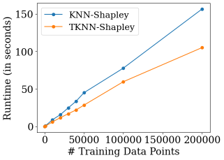
We evaluate the runtime efficiency of TKNN-Shapley in comparison to KNN-Shapley (see Appendix E.2 for details as well as more experiments). We choose a range of training data sizes $N$, and compare the runtime of both methods at each $N$. As demonstrated in Figure 2, TKNN-Shapley achieves better computational efficiency than KNN-Shapley across all training data sizes. In particular, TKNN-Shapley is around 30% faster than KNN-Shapley for large $N$. This shows the computational advantage of TKNN-Shapley mentioned in Section 4.2.

In this section, we evaluate the performance of both DP and non-DP version of TKNN-Shapley in discerning data quality. Tasks: We evaluate the performance of TKNN-Shapley on two standard tasks: mislabeled data detection and noisy data detection, which are tasks that are often used for evaluating the performance of data valuation techniques in prior works [KZ22, WJ23a]. Since mislabeled/noisy data often negatively affect the model performance, it is desirable to assign low values to these data points. In the experiment of mislabeled (or noisy) data detection, we randomly choose 10% of the data points and flip their labels (or add strong noise to their features). Datasets: We conduct our experiments on a diverse set of 13 datasets, where 11 of them have been used in previous data valuation studies [KZ22, WJ23a]. Additionally, we experiment on 2 NLP datasets (AG News [WSZY21] and DBPedia [ABK⁺07]) that have been rarely used in the past due to their high-dimensional nature and the significant computational resources required. Settings & Hyperparameters of TKNN-/KNN-Shapley: for both TKNN/KNN-Shapley, we use the popular cosine distance as the distance measure [Raj21], which is always bounded in $[-1,+1]$. Throughout all experiments, we use $\tau=-0.5$ and $K=5$ for TKNN-/KNN-Shapley, respectively, as we found the two choices consistently work well across all datasets. We conduct ablation studies on the choice of hyperparameters in Appendix E.

References

- [ABK+07] Sören Auer, Christian Bizer, Georgi Kobilarov, Jens Lehmann, Richard Cyganiak, and Zachary Ives. Dbpedia: A nucleus for a web of open data. In The Semantic Web: 6th International Semantic Web Conference, 2nd Asian Semantic Web Conference, ISWC 2007+ ASWC 2007, Busan, Korea, November 11-15, 2007. Proceedings, pages 722–735. Springer, 2007.
- [ACG+16] Martin Abadi, Andy Chu, Ian Goodfellow, H Brendan McMahan, Ilya Mironov, Kunal Talwar, and Li Zhang. Deep learning with differential privacy. In Proceedings of the 2016 ACM SIGSAC conference on computer and communications security, pages 308–318, 2016.
- [BBG18] Borja Balle, Gilles Barthe, and Marco Gaboardi. Privacy amplification by subsampling: Tight analyses via couplings and divergences. Advances in Neural Information Processing Systems, 31, 2018.
- [BC21] Mark Alexander Burgess and Archie C Chapman. Approximating the shapley value using stratified empirical bernstein sampling. In IJCAI, pages 73–81, 2021.
- [Ben75] Jon L Bentley. Survey of techniques for fixed radius near neighbor searching. Technical report, Stanford Linear Accelerator Center, Calif.(USA), 1975.
- [BPS19] Eugene Bagdasaryan, Omid Poursaeed, and Vitaly Shmatikov. Differential privacy has disparate impact on model accuracy. Advances in neural information processing systems, 32, 2019.
- [BRX+21] Yatao Bian, Yu Rong, Tingyang Xu, Jiaxiang Wu, Andreas Krause, and Junzhou Huang. Energy-based learning for cooperative games, with applications to valuation problems in machine learning. arXiv preprint arXiv:2106.02938, 2021.
- [CCN+22] Nicholas Carlini, Steve Chien, Milad Nasr, Shuang Song, Andreas Terzis, and Florian Tramer. Membership inference attacks from first principles. In 2022 IEEE Symposium on Security and Privacy (SP), pages 1897–1914. IEEE, 2022.
- [CEP+23] Rachel Cummings, Hadi Elzayn, Emmanouil Pountourakis, Vasilis Gkatzelis, and Juba Ziani. Optimal data acquisition with privacy-aware agents. In 2023 IEEE Conference on Secure and Trustworthy Machine Learning (SaTML), pages 210–224. IEEE, 2023.
- [CS21] Christie Courtnage and Evgueni Smirnov. Shapley-value data valuation for semi-supervised learning. In Discovery Science: 24th International Conference, DS 2021, Halifax, NS, Canada, October 11–13, 2021, Proceedings 24, pages 94–108. Springer, 2021.
- [DKM+06] Cynthia Dwork, Krishnaram Kenthapadi, Frank McSherry, Ilya Mironov, and Moni Naor. Our data, ourselves: Privacy via distributed noise generation. In Advances in Cryptology-EUROCRYPT 2006: 24th Annual International Conference on the Theory and Applications of Cryptographic Techniques, St. Petersburg, Russia, May 28-June 1, 2006. Proceedings 25, pages 486–503. Springer, 2006.
- [DMNS06] Cynthia Dwork, Frank McSherry, Kobbi Nissim, and Adam Smith. Calibrating noise to sensitivity in private data analysis. In Theory of cryptography conference, pages 265–284. Springer, 2006.
- [DN03] Irit Dinur and Kobbi Nissim. Revealing information while preserving privacy. In Proceedings of the twenty-second ACM SIGMOD-SIGACT-SIGART symposium on Principles of database systems, pages 202–210, 2003.
- [DNW81] Pradeep Dubey, Abraham Neyman, and Robert James Weber. Value theory without efficiency. Mathematics of Operations Research, 6(1):122–128, 1981.
- [DPCJB15] Andrea Dal Pozzolo, Olivier Caelen, Reid A Johnson, and Gianluca Bontempi. Calibrating probability with undersampling for unbalanced classification. In 2015 IEEE Symposium Series on Computational Intelligence, pages 159–166. IEEE, 2015.
- [DR+14] Cynthia Dwork, Aaron Roth, et al. The algorithmic foundations of differential privacy. Foundations and Trends® in Theoretical Computer Science, 9(3–4):211–407, 2014.
- [DR16] Cynthia Dwork and Guy N. Rothblum. Concentrated differential privacy. CoRR, abs/1603.01887, 2016.
- [DRV10] Cynthia Dwork, Guy N Rothblum, and Salil Vadhan. Boosting and differential privacy. In 2010 IEEE 51st Annual Symposium on Foundations of Computer Science, pages 51–60. IEEE, 2010.
- [DSSU17] Cynthia Dwork, Adam Smith, Thomas Steinke, and Jonathan Ullman. Exposed! a survey of attacks on private data. Annual Review of Statistics and Its Application, 4:61–84, 2017.
- [FMMO22] Alireza Fallah, Ali Makhdoumi, Azarakhsh Malekian, and Asuman Ozdaglar. Optimal and differentially private data acquisition: Central and local mechanisms. In Proceedings of the 23rd ACM Conference on Economics and Computation, pages 1141–1141, 2022.
- [GHV20] Marco Gaboardi, Michael Hay, and Salil Vadhan. A programming framework for opendp. Manuscript, May, 2020.
- [GKKW02] László Györfi, Michael Köhler, Adam Krzyżak, and Harro Walk. A distribution-free theory of nonparametric regression, volume 1. Springer, 2002.
- [GKZ20] Amirata Ghorbani, Michael Kim, and James Zou. A distributional framework for data valuation. In International Conference on Machine Learning, pages 3535–3544. PMLR, 2020.
- [GLW21] Sivakanth Gopi, Yin Tat Lee, and Lukas Wutschitz. Numerical composition of differential privacy. Advances in Neural Information Processing Systems, 34:11631–11642, 2021.
- [GZ19] Amirata Ghorbani and James Zou. Data shapley: Equitable valuation of data for machine learning. In International Conference on Machine Learning, pages 2242–2251. PMLR, 2019.
- [GZE22] Amirata Ghorbani, James Zou, and Andre Esteva. Data shapley valuation for efficient batch active learning. In 2022 56th Asilomar Conference on Signals, Systems, and Computers, pages 1456–1462. IEEE, 2022.
- [HZRS16] Kaiming He, Xiangyu Zhang, Shaoqing Ren, and Jian Sun. Deep residual learning for image recognition. In Proceedings of the IEEE conference on computer vision and pattern recognition, pages 770–778, 2016.
- [IK19] Ferenc Illés and Péter Kerényi. Estimation of the shapley value by ergodic sampling. arXiv preprint arXiv:1906.05224, 2019.
- [JDW+19a] Ruoxi Jia, David Dao, Boxin Wang, Frances Ann Hubis, Nezihe Merve Gurel, Bo Li, Ce Zhang, Costas J Spanos, and Dawn Song. Efficient task-specific data valuation for nearest neighbor algorithms. Proceedings of the VLDB Endowment, 2019.
- [JDW+19b] Ruoxi Jia, David Dao, Boxin Wang, Frances Ann Hubis, Nick Hynes, Nezihe Merve Gürel, Bo Li, Ce Zhang, Dawn Song, and Costas J Spanos. Towards efficient data valuation based on the shapley value. In The 22nd International Conference on Artificial Intelligence and Statistics, pages 1167–1176. PMLR, 2019.
- [JWS+21] Ruoxi Jia, Fan Wu, Xuehui Sun, Jiacen Xu, David Dao, Bhavya Kailkhura, Ce Zhang, Bo Li, and Dawn Song. Scalability vs. utility: Do we have to sacrifice one for the other in data importance quantification? In Proceedings of the IEEE/CVF Conference on Computer Vision and Pattern Recognition, pages 8239–8247, 2021.
- [KDI+22] Bojan Karlaš, David Dao, Matteo Interlandi, Bo Li, Sebastian Schelter, Wentao Wu, and Ce Zhang. Data debugging with shapley importance over end-to-end machine learning pipelines. arXiv preprint arXiv:2204.11131, 2022.
- [KH+09] Alex Krizhevsky, Geoffrey Hinton, et al. Learning multiple layers of features from tiny images. 2009.
- [KH21] Antti Koskela and Antti Honkela. Computing differential privacy guarantees for heterogeneous compositions using fft. CoRR, abs/2102.12412, 2021.
- [KJH20] Antti Koskela, Joonas Jälkö, and Antti Honkela. Computing tight differential privacy guarantees using fft. In International Conference on Artificial Intelligence and Statistics, pages 2560–2569. PMLR, 2020.
- [KL17] Pang Wei Koh and Percy Liang. Understanding black-box predictions via influence functions. In International Conference on Machine Learning, pages 1885–1894. PMLR, 2017.
- [KPR23] Justin Kang, Ramtin Pedarsani, and Kannan Ramchandran. The fair value of data under heterogeneous privacy constraints. arXiv preprint arXiv:2301.13336, 2023.
- [KPRU14] Michael Kearns, Mallesh Pai, Aaron Roth, and Jonathan Ullman. Mechanism design in large games: Incentives and privacy. In Proceedings of the 5th conference on Innovations in theoretical computer science, pages 403–410, 2014.
- [KZ22] Yongchan Kwon and James Zou. Beta shapley: a unified and noise-reduced data valuation framework for machine learning. In International Conference on Artificial Intelligence and Statistics, pages 8780–8802. PMLR, 2022.
- [KZ23] Yongchan Kwon and James Zou. Data-oob: Out-of-bag estimate as a simple and efficient data value. ICML, 2023.
- [LeC98] Yann LeCun. The mnist database of handwritten digits. http://yann. lecun. com/exdb/mnist/, 1998.
- [LJX22] Xinjian Luo, Yangfan Jiang, and Xiaokui Xiao. Feature inference attack on shapley values. In Proceedings of the 2022 ACM SIGSAC Conference on Computer and Communications Security, pages 2233–2247, 2022.
- [LLL+21] Jinfei Liu, Jian Lou, Junxu Liu, Li Xiong, Jian Pei, and Jimeng Sun. Dealer: an end-to-end model marketplace with differential privacy. Proceedings of the VLDB Endowment, 14(6), 2021.
- [LLY21] Weixin Liang, Kai-Hui Liang, and Zhou Yu. Herald: An annotation efficient method to detect user disengagement in social conversations. In Proceedings of the 59th Annual Meeting of the Association for Computational Linguistics and the 11th International Joint Conference on Natural Language Processing (Volume 1: Long Papers), pages 3652–3665, 2021.
- [LSL17] Min Lyu, Dong Su, and Ninghui Li. Understanding the sparse vector technique for differential privacy. Proceedings of the VLDB Endowment, 10(6), 2017.
- [LZL+22] Jinkun Lin, Anqi Zhang, Mathias Lécuyer, Jinyang Li, Aurojit Panda, and Siddhartha Sen. Measuring the effect of training data on deep learning predictions via randomized experiments. In International Conference on Machine Learning, pages 13468–13504. PMLR, 2022.
- [LZY20] Weixin Liang, James Zou, and Zhou Yu. Beyond user self-reported likert scale ratings: A comparison model for automatic dialog evaluation. In Proceedings of the 58th Annual Meeting of the Association for Computational Linguistics, pages 1363–1374, 2020.
- [MCFH22] Rory Mitchell, Joshua Cooper, Eibe Frank, and Geoffrey Holmes. Sampling permutations for shapley value estimation. 2022.
- [NS06] Arvind Narayanan and Vitaly Shmatikov. How to break anonymity of the netflix prize dataset. arXiv preprint cs/0610105, 2006.
- [OL21] Ramin Okhrati and Aldo Lipani. A multilinear sampling algorithm to estimate shapley values. In 2020 25th International Conference on Pattern Recognition (ICPR), pages 7992–7999. IEEE, 2021.
- [Ope23] OpenAI. Planning for agi and beyond, 2023.
- [PFTS21] Konstantin D Pandl, Fabian Feiland, Scott Thiebes, and Ali Sunyaev. Trustworthy machine learning for health care: scalable data valuation with the shapley value. In Proceedings of the Conference on Health, Inference, and Learning, pages 47–57, 2021.
- [Raj21] Sabita Rajbanshi. Chapter 1: K nearest neighbors (supervised machine learning algorithm), 2021.
- [RG19] Nils Reimers and Iryna Gurevych. Sentence-bert: Sentence embeddings using siamese bert-networks. In Proceedings of the 2019 Conference on Empirical Methods in Natural Language Processing. Association for Computational Linguistics, 11 2019.
- [Sha53] Lloyd S Shapley. A value for n-person games. Contributions to the Theory of Games, 2(28):307–317, 1953.
- [SMJ+21] Dongsub Shim, Zheda Mai, Jihwan Jeong, Scott Sanner, Hyunwoo Kim, and Jongseong Jang. Online class-incremental continual learning with adversarial shapley value. In Proceedings of the AAAI Conference on Artificial Intelligence, volume 35, pages 9630–9638, 2021.
- [SS98] Pierangela Samarati and Latanya Sweeney. Protecting privacy when disclosing information: k-anonymity and its enforcement through generalization and suppression. 1998.
- [SSSS17] Reza Shokri, Marco Stronati, Congzheng Song, and Vitaly Shmatikov. Membership inference attacks against machine learning models. In 2017 IEEE symposium on security and privacy (SP), pages 3–18. IEEE, 2017.
- [TLL+22] Zhihua Tian, Jian Liu, Jingyu Li, Xinle Cao, Ruoxi Jia, and Kui Ren. Private data valuation and fair payment in data marketplaces. arXiv preprint arXiv:2210.08723, 2022.
- [War19] Mark Warner. Warner & hawley introduce bill to force social media companies to disclose how they are monetizing user data, 2019.
- [WAYS22] Lauren Watson, Rayna Andreeva, Hao-Tsung Yang, and Rik Sarkar. Differentially private shapley values for data evaluation. arXiv preprint arXiv:2206.00511, 2022.
- [Wei] Cynthia Weiss. Mayo clinic platform: A patient’s experience and beyond.
- [WJ23a] Jiachen T Wang and Ruoxi Jia. Data banzhaf: A robust data valuation framework for machine learning. In International Conference on Artificial Intelligence and Statistics, pages 6388–6421. PMLR, 2023.
- [WJ23b] Jiachen T Wang and Ruoxi Jia. A note on" efficient task-specific data valuation for nearest neighbor algorithms". arXiv preprint arXiv:2304.04258, 2023.
- [WJ23c] Jiachen T Wang and Ruoxi Jia. A note on" towards efficient data valuation based on the shapley value”. arXiv preprint arXiv:2302.11431, 2023.
- [WRZ+20] Tianhao Wang, Johannes Rausch, Ce Zhang, Ruoxi Jia, and Dawn Song. A principled approach to data valuation for federated learning. In Federated Learning, pages 153–167. Springer, 2020.
- [WSL22] Zhaoxuan Wu, Yao Shu, and Bryan Kian Hsiang Low. Davinz: Data valuation using deep neural networks at initialization. In International Conference on Machine Learning, pages 24150–24176. PMLR, 2022.
- [WSZY21] Zhen Wang, Xu Shan, Xiangxie Zhang, and Jie Yang. N24news: A new dataset for multimodal news classification. arXiv preprint arXiv:2108.13327, 2021.
- [WYJ22] Tianhao Wang, Yu Yang, and Ruoxi Jia. Improving cooperative game theory-based data valuation via data utility learning. ICLR 2022 Workshop on Socially Responsible Machine Learning, 2022.
- [Yao82] Andrew C Yao. Protocols for secure computations. In 23rd annual symposium on foundations of computer science (sfcs 1982), pages 160–164. IEEE, 1982.
- [YL09] I-Cheng Yeh and Che-hui Lien. The comparisons of data mining techniques for the predictive accuracy of probability of default of credit card clients. Expert systems with applications, 36(2):2473–2480, 2009.
- [ZZGW23] Yuqing Zhu, Xuandong Zhao, Chuan Guo, and Yu-Xiang Wang. Private prediction strikes back! Private kernelized nearest neighbors with individual Rényi filter. In Proceedings of the Thirty-Ninth Conference on Uncertainty in Artificial Intelligence, pages 2586–2596, 2023.
Appendix A Extended Related Work
KNN-Shapley & Its Applications.
The Shapley value is known for being computationally expensive. Fortunately, [JDW+19a] found that computing the Data Shapley for K-Nearest Neighbors (KNN), one of the most classic yet still popular ML algorithms, is surprisingly easy and efficient. To the best of our knowledge, unweighted KNN is the only commonly-used ML model for which the exact Data Shapley can be efficiently computed, referred to as ‘KNN-Shapley’. Owing to its superior computational efficiency and effectiveness in distinguishing data quality, KNN-Shapley has become one of the most popular and practical data valuation techniques. In the realm of ML research, for instance, [GZE22] extends KNN-Shapley to active learning, [SMJ+21] employs it in a continual learning setting, [LZY20, LLY21] utilize KNN-Shapley for removing confusing samples in NLP applications, and [CS21] adopts KNN-Shapley for data valuation in semi-supervised learning. Furthermore, KNN-Shapley has also proven to be highly practical in real-life applications: [PFTS21] demonstrates that KNN-Shapley is the only practical data valuation technique for valuing large amounts of healthcare data, and [KDI+22] builds the first data debugging system for end-to-end ML pipelines based on KNN-Shapley.
Remark 5 (KNN-Shapley vs General Data Shapley).
In comparison to the work of general Data Shapley [GZ19] (including Beta Shapley [KZ22] as well as Data Banzhaf [WJ23a]), KNN-Shapley may have the following differences: (1) KNN-Shapley focuses on KNN classifiers. As a result, the applicability of KNN-Shapley scores as a proxy of data points’ value with respect to other ML models may not be straightforward. However, it is noteworthy that KNN is asymptotically Bayes optimal, implying that KNN-Shapley scores can be justified as a proxy for the data’s value relative to the best possible model, i.e., the Bayes classifier, under certain asymptotic conditions. (2) For high-dimensional data, such as images, KNN-Shapley requires a public model to first map the original data into data embeddings, and evaluates the value of these embeddings rather than the original data. While this is indeed a constraint in certain scenario, it is important to recognize that utilizing a publicly available foundation model to convert original data into embeddings, followed by the fine-tuning of the model’s last layer, has become a common practice. Therefore, in many situations, it might be more desirable to evaluate the value of data embeddings instead of the original data.
Privacy and Data Valuation.
Few studies in the literature consider the privacy risks of data valuation. [TLL+22] explores a scenario where a trusted server does not exist, and different data holders collaboratively compute each other’s Shapley values without actually examining the data holder’s data points, utilizing Multi-party Computation (MPC) techniques. The privacy risks addressed in [TLL+22] are orthogonal to those in our paper, and we can combine both techniques for end-to-end privacy protection. Another orthogonal line of works [LLL+21, FMMO22, CEP+23, KPR23] studies the scenario of a central platform collecting private data from privacy-aware agents and offering a differentially private statistic computed from the submitted data as a service in return. Agents consider the privacy costs and benefits of obtaining the statistic when deciding whether to participate and reveal their data truthfully. [LJX22] proposes a privacy attack on the Shapley value for feature attribution, while in this work we study the privacy risks when using the Shapley value for data valuation.
The unpublished manuscript by [WAYS22] is the work most closely related to ours. [WAYS22] explores how to make the Shapley values of a data point to be differentially private against the rest of the dataset. However, instead of focusing on KNN-Shapley, they study the privatization of the less practical, retrain-based Data Shapley [GZ19, JDW+19b]. Furthermore, their algorithm is highly restrictive in that the differential privacy guarantee relies on the "uniform stability" assumption, which is not verifiable for modern learning algorithms such as neural networks. Moreover, while [WAYS22] argues the "uniform stability" assumption holds for Logistic regression on bounded data domain, it is unclear whether the uniform stability assumption still holds when the Logistic regression is trained by SGD (which may involve training stochasticity and early stopping). In addition, [WAYS22] does not release the implementation. Hence, in our experiment, we do not compare with it.
Remark 6 (Brief background for the privacy risks in releasing aggregated statistics).
Since 1998, researchers have observed that a lot of seemingly benevolent aggregate statistics of a dataset can be used to reveal sensitive information about individuals [SS98]. A classic example is Netflix Prize fiasco, where the researchers show that an anonymized dataset can leak many sensitive information about individuals [NS06]. Dinur and Nissim [DN03] proved that “revealing too many statistics too accurately leads to data privacy breach”. A great amount of discussion and practical realization of these privacy attacks on aggregated statistics can be found in [DSSU17]. In 2020, the US Census Bureau used these privacy attacks to justify its use of differential privacy.
KNN-Shapley score for an individual is one kind of aggregated statistic that depends on the rest of the dataset. Hence, KNN-Shapley score intrinsically reveals private information about the rest of the dataset (where we use membership inference attack as a concrete example in our paper). In addition, when users collude, their KNN-shapley values can be combined to make joint inferences about the rest of the dataset.
Appendix B Details about KNN-Shapley, its Privacy Risks & Challenges of Privatization
B.1 Full version of KNN-Shapley
KNN-Shapley was originally proposed in [JDW+19a] and was later refined in [WJ23b]. Specifically, [WJ23b] considers the KNN’s utility function formula (2) we present in the main text. Here is the main result of [WJ23b]:
Theorem 7 (KNN-Shapley [WJ23b]).
Consider the utility function in (2). Given a validation data point and a distance metric , if we sort the training set according to in ascending order, then the Shapley value of each data point corresponding to utility function can be computed recursively as follows:
where denotes the number of classes for the classification task.
B.1.1 Older version of KNN-Shapley from [JDW+19a]
Prior to the current formulation of KNN-Shapley introduced by [WJ23b], [JDW+19a] proposed an older version of the algorithm. There is only a small distinction between the updated version by [WJ23b] and the older version from [JDW+19a]. Specifically, the difference between the versions proposed by [WJ23b] and [JDW+19a] lies in the utility function considered when computing the Shapley value. [WJ23b] use the utility function (2) as presented in the main text, while the utility function used in [JDW+19a] is slightly less interpretable: