Threshold for a Discrete-Variable Sensor of Quantum Reservoirs
Abstract
Quantum sensing employs quantum resources of a sensor to attain a smaller estimation error of physical quantities than the limit constrained by classical physics. To measure a quantum reservoir, which is significant in decoherence control, a nonunitary-encoding sensing scheme becomes necessary. However, previous studies showed that the reservoir-induced degradation to quantum resources of the sensor makes the errors divergent with the increase of encoding time. We here propose a scheme to use two-level systems as the sensor to measure a quantum reservoir. A threshold, above which the shot-noise-limited sensing error saturates or even persistently decreases with the encoding time, is uncovered. Our analysis reveals that it is due to the formation of a bound state of the total sensor-reservoir system. Solving the outstanding error-divergency problem in previous studies, our result supplies an insightful guideline in realizing a sensitive measurement of quantum reservoirs.
I Introduction
Quantum sensing aims at achieving a highly precise measurement to physical quantities with the help of quantum resources of a sensor Degen et al. (2017). The sensing error governed by classical physics is constrained by the so-called shot-noise limit (SNL) Caves (1981). It has been demonstrated that the SNL can be beaten by using quantum entanglement Pezzè et al. (2018); Zhang et al. (2018); Nagata et al. (2007) and squeezing Evrard et al. (2019); Haine and Hope (2020); Muessel et al. (2014); Nolan et al. (2017). Many fantastic applications of quantum sensing have been made in gravitational-wave detection Tse et al. (2019); Acernese et al. (2019), quantum radar Maccone and Ren (2020), atom clocks Kessler et al. (2014); Mehlstäubler et al. (2018), magnetometers Potts et al. (2019); Bouton et al. (2020); Troiani and Paris (2018); Razzoli et al. (2019), and thermometries Cavina et al. (2018); Hovhannisyan and Correa (2018). A common feature of these applications is that the quantities of interest are encoded into the sensor state via a unitary dynamics Huelga et al. (1997); Caves (1981); Wang et al. (2019); Chabuda et al. (2020); Gessner et al. (2019); Gatto et al. (2019); Yu et al. (2020); Zhuang and Zhang (2019); Kura and Ueda (2020); Che et al. (2019). Such unitary-encoding scheme is applicable only in measuring the quantities of classical systems. When the ones of a quantum system are measured, the sensor-system coupling for quantity encoding inevitably results in a nonunitary dynamics of the sensor. How do we generalize the well-developed unitary-encoding sensing scheme to the nonunitary case and achieve a highly precise sensing of quantum systems in the nonunitary-encoding setting?
Recently, much attention has been focused on precisely measuring quantum reservoirs Chen et al. (2020); Goldwater et al. (2019); Mascherpa et al. (2017); Xu et al. (2019); Farfurnik and Bar-Gill (2020); Benedetti et al. (2018); Bina et al. (2018); Tamascelli et al. (2020); Sehdaran et al. (2019a, b). The coupling of the reservoir to any microscopic system would cause the system to lose its quantum coherence, which is called decoherence. Controlling the detrimental impacts of decoherence on the relevant system is crucial in realizing quantum information processing and many other quantum technologies Li et al. (2018); Breuer et al. (2016); de Vega and Alonso (2017); Rivas et al. (2014); Streltsov et al. (2017); Li et al. (2018). Decoherence is essentially determined by the spectral density of the reservoir, which characterizes the system-reservoir coupling strength per unit frequency of the reservoir. Therefore, the grasping of the feature of the spectral density is a prerequisite for decoherence control Kofman and Kurizki (2001); Soare et al. (2014). However, in many occasions, the spectral density cannot be microscopically derived from first principle. Thus, a precise sensing to the spectral density of quantum reservoir is strongly necessary Chen et al. (2020); Goldwater et al. (2019); Mascherpa et al. (2017); Xu et al. (2019); Farfurnik and Bar-Gill (2020). Several nonunitary-encoding schemes of sensing the quantum reservoir have been proposed. Unfortunately, as shown in previous works Benedetti et al. (2018); Bina et al. (2018); Tamascelli et al. (2020); Sehdaran et al. (2019a, b), although the nonunitary dynamics can successfully encode the spectral density into the sensor state, it meanwhile erases the quantum resource attached to the sensor, which causes the sensing error to become larger and larger with the increase of encoding time. Thus, solving the error-divergency problem in the long-encoding-time regime still remains as an open question and is necessary for any scheme to sense a quantum reservoir.
In this work, using two-level systems (TLSs) as the sensor, we propose a nonunitary-encoding sensing scheme to estimate the spectral density of a quantum reservoir. Going beyond the widely used pure-dephasing coupling and the Born-Markovian approximation, we exactly study the performance of an initial product and a Greenberger-Horne-Zeilinger (GHZ) entangled state of the sensor on the estimation error via the dissipative interactions for encoding. A threshold, above which the sensing error decreases with the encoding time as for the initial product state and saturates to a finite value with the encoding time for the entangled state, is found. This is in sharp contrast to the error-divergency result in the previous works. Further study reveals that it is due to the formation of a bound state of the composite system consisting of each TLS and the reservoir. Supplying an efficient way to eliminate the longstanding error-divergency problem in sensing a quantum reservoir by manipulating the formation of the bound state, our scheme can be used to realize a SNL-type estimation to the spectral density of the quantum reservoir.
II Quantum parameter estimation
A quantum sensing scheme generally contains the steps of initial-state preparation, parameter encoding, and measurements. To sense a quantity of certain physical system, one first prepares a well-tailored quantum sensor in an initial state . The sensed quantity is encoded into the sensor state via coupling the sensor to the physical system. Finally, one measures a chosen physical observable of the sensor and infers the value of from the measurement results. In any quantum sensing process, one cannot completely eliminate the errors and estimate the quantity of interest precisely. According to quantum parameter-estimation theory Liu et al. (2019), whatever the observable is measured, the ultimate estimation error of is constrained by the famous quantum Cramér-Rao bound . Here is the root mean square as the error of , is the number of repeated measurements which is set to 1 in this work for explicitness, and , with being determined by , is quantum Fisher information (QFI) describing the most information of contained in . It can be readily found that the minimal sensing error is completely determined by the QFI: a larger QFI always means a smaller estimation error. Maximizing the value of QFI by optimizing the quantum resource in and the sensor-system interaction is the major objective of quantum sensing. When , or equivalently, , with being the total particle number in the sensor, such scaling relation is called SNL. It has been demonstrated that the SNL can be surpassed by using entanglement Giovannetti et al. (2004, 2006); Bollinger et al. (1996); Huelga et al. (1997); Daryanoosh et al. (2018), by the encoding process via quantum criticality Frérot and Roscilde (2018); Rams et al. (2018), and by using nonlinear interactions Chen et al. (2018).
III Quantum sensing of a dissipative reservoir
In order to precisely sense a quantum reservoir, we employ identical TLSs as the sensor. The information of the reservoir is encoded into the sensor via the individual interactions of each TLS with the reservoir described by the following Hamiltonian ():
| (1) |
where is the ladder operators between the ground state and excited state of the th TLS with frequency , denotes the annihilation operator of the th mode with frequency of the reservoir coupled to the th TLS, and denote their coupling strengths. The specific properties of the reservoir is described by its spectral density , which in turn determines the decoherence effect caused by this reservoir to any quantum system.
Assuming the sensor-reservoir coupling is switched on at the initial time, thus we have the initial state of the total system as with and being the initial sate of the sensor and the reservoirs, respectively. After tracing out the degrees of freedom of the reservoirs, we find that the dynamics of the sensor is governed by the non-Markovian master equation Wang et al. (2017)
| (2) |
where describes the dissipation induced by reservoirs, is the renormalized frequency of the th TLS and denotes the dissipation rate. Here, is determined by the integro-differential equation
| (3) |
with and . It can be seen that the information of the reservoir characterized by the spectral density has been successfully encoded in the sensor state via the master equation (2).
It should be emphasized that, different from the widely used unitary evolution, the parameter encoding governed by Eq. (2) is a nonunitary dynamics of the sensor. Such nonunitary dynamics in turn causes decoherence to the sensor, which destroys the quantum resource carried by the sensor. Therefore, balancing the necessary parameter-encoding process and the decoherence effect in the nonunitary dynamics is crucial in achieving the high precision of our sensing scheme. Taking the Ohmic-family spectral density as an example, we explore the performance of our sensing scheme to the reservoir. Here is a dimensionless coupling constant, is a cutoff frequency, and is the so-called Ohmicity parameter. Depending on the value of , a quantum reservoir can be classified into three categories: a sub-Ohmic reservoir (), an Ohmic reservoir (), and a super-Ohmic reservoir () Leggett et al. (1987). In this paper, , , and are the quantities to be estimated.
We consider two different initial states: an uncorrelated state and a GHZ-type maximally entangled state . The solution of the master equation (2) can be expressed in the Kraus representation as with , where and with Wang et al. (2017); Ma et al. (2011); Tan et al. (2013). We can derive the reduced density matrix of the sensor for the two initial states as
| (4) | |||||
| (5) | |||||
After some algebra (see Appendix A), we obtain the QFI of as
| (6) |
where being the Bloch vector and . The one of is with (see Appendix A)
| (7) | |||
| (8) |
where , , and .
In the special case when the sensor-reservoir coupling is weak and the characteristic time scale of the reservoir is smaller than that of the sensor, we can safely apply the Markovian approximation to Eq. (3). Under this approximation, we have Yang et al. (2014), where determines the decay rate and is a frequency shift induced by the reservoirs. Substituting the above approximate into Eqs. (4) and (5), one can immediately find
| (9) |
Due to the fact that this long-time steady state does not contain any information about the spectral density, we can conclude that and corresponding sensing error becomes divergent in the long-encoding-time regime. Such an error-divergence problem has been reported in previous works Benedetti et al. (2018); Bina et al. (2018); Tamascelli et al. (2020); Sehdaran et al. (2019a, b), which severely restricts the realization of precisely sensing the quantum reservoir.
IV Threshold of the sensitivity
In the non-Markovian case, one needs to numerically solve Eq. (3) to obtain the QFI. However, before performing these numerical simulations, we would like to use the Laplace transformation to analyze the long-time dynamical behavior of , which can provide some qualitative results and is benefit for us to establish a clear physical picture. Applying Laplace transformation on Eq. (3), one can find . The expression of can be derived by using the Cauchy residue theorem via finding the poles of from
| (10) |
It can be proven that the roots of Eq. (10) are just the eigenenergies of the single sensor-reservoir Hamiltonian in the single-excitation subspace Tong et al. (2010). Therefore, the dynamical behavior of is closely associated with the feature of the energy spectrum of the sensor-reservoir system. Since is a monotonically decreasing function in the regime , Eq. (10) has only one isolated root provided . We call the eigenstate corresponding to this isolated eigenenergy the bound state. In contrast, Eq. (10) has infinite roots in the regime , which form a continuous energy band. With the help of the above analysis, the inverse Laplace transform can be exactly done, which results in
| (11) |
with . The first term in Eq. (11) is contributed by the potentially formed bound state, while the second term is from the continuous band energies. The second term gradually vanishes with time due to out-of-phase interference. Thus, if a bound state is formed, then , leading a dissipationless dynamics; while if the bound state is absent, then , which characterizes a complete decoherence. For the Ohmic-family spectral density considered in this paper, the criterion of forming a bound state can be analytically expressed as Yang et al. (2014), where is Euler’s function.
Due to the fact that in the absence of the bound state, our sensing scheme is then qualitatively consistent with the Markovian case, in which the sensing error diverges in the long-encoding-time regime irrespective of whether the initial state is the product state or the GHZ state. In the presence of the bound state, substituting the long-time form into Eqs. (6), (7), and (8), we find that the long-time asymptotic QFI in the large- limit are given by (see Appendix A)
| (12) | |||||
| (13) |
It is remarkable to see from the above expression that the QFI behaves as when the initial state is the uncorrelated state. This result implies the sensing error can be continuously diminished by prolonging the encoding time, i.e., . Such a time-scaling relation is the same as the noiseless Ramsey-spectroscopy metrology scheme Huelga et al. (1997); Wang et al. (2017). It means that, much different from the previous work Benedetti et al. (2018); Bina et al. (2018); Tamascelli et al. (2020); Sehdaran et al. (2019a, b) and the Markovian approximate case, the encoding time in our scheme can be used as a resource to improve the sensing precision, which is similar to the widely used unitary-encoding scheme in the ideal case. On the other hand, if the initial state is the GHZ state, the QFI ultimately approaches a nonzero steady value. It is not a surprise that the product state outperforms the GHZ state in taking the encoding time as a resource because the entanglement contained in the GHZ state is fragile to the local decoherence. The resource of multipartite entanglement carried by the GHZ state has already been destroyed at the early evolution and cannot show its superiority in the long-time regime. Even so, both of the above results are completely different from the Markovian approximate result in which the QFI vanishes in the long-encoding-time regime. The bound state favored nonzero QFI in the long-time limit can be understood as follows. As a stationary state of the total system, the bound state is immune to the reservoir-induced decoherence. Therefore, the messages of spectral density encoded in the bound state is preserved and thus a nonzero QFI is achieved in the long-time limit. This sufficiently solves the error-divergency problem. Another result revealed by Eqs. (12) and (13) is that the sensing precision scales with the number of the TLSs as the SNL in the large- limit. This result once again exhibits the advantage of our scheme over the Markovian approximate one, in which the SNL is totally destroyed in the long-time limit. It is noted that the distinguished roles played by the bound state in continuous-variable sensor Wu et al. (2021) and the Mech-Zehnder-interferometry-based quantum metrology Bai et al. (2019) have been reported.
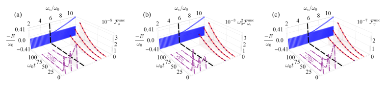
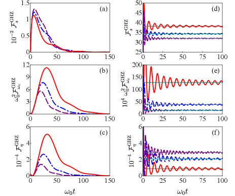
To verify the above analytical results, we present the numerical calculations on the QFI as the function of in Figs. 1 and 2. We can see that the QFI exhibits a similar behavior in the regime where the bound state is absent regardless of whether the initial state is the uncorrelated or GHZ states. At the beginning, the QFI gradually increases from its initial value to the maximal values. Then the QFI begins to decrease and eventually disappears in the long-encoding-time limit. This numerical result is consistent with many previous studies Benedetti et al. (2018); Bina et al. (2018); Tamascelli et al. (2020); Sehdaran et al. (2019a, b). In sharp contrast to this, when the bound state is present, the QFI for the uncorrelated state exhibits a square power-law increase with the encoding time (see Fig. 1), while the one for the GHZ state saturates to a nonzero value [see Figs. 2(d), 2(e), and 2(f)]. The numerical results in both Figs. 1 and 2 are in good agreement with our analytical Eqs. (12) and (13) in the long-time limit, which validates our analytical results. It is noted that, although only the large- case is studied, the constructive role of the bound state in enhancing the sensing sensitivity is also valid in the small- case (see Appendix B).
V Discussion and conclusions
It is necessary to point out that our sensing scheme is independent of the explicit form of the spectral density. Although only the Ohmic-family spectral densities are displayed in this paper, our sensing scheme can be generalized to other cases without difficulty. For non-Ohmic-family cases, the specific condition of forming a bound state might be quantitatively different, but the effectiveness of our scheme remains unchanged. Recently, the observation of the bound-state effect, which is the key recipe in our scheme, has been reported in circuit quantum electrodynamics architecture Liu and Houck (2017) as well as matter-wave systems Krinner et al. (2018). These experimental achievements provide a strong support to our sensing scheme and indicate that our finding is realizable by employing the experimental technique of quantum optics.
In summary, using TLSs as a sensor, we present a nonunitary-encoding sensing scheme to estimate the spectral density of a quantum reservoir. A mechanism to overcome the outstanding error-divergence problem in the literature is revealed. It is found that, accompanying the formation of a TLS-reservoir bound state, the shot-noise-limited estimation error saturates to a finite value for the GHZ-type entangled state and persistently decreases for the product state with the encoding time. An analytical threshold to achieve this amazing result is given explicitly. Our result supplies an insightful guideline to practically realize the sensing to the quantum reservoir and may have a deep impact on controlling the reservoir-induced decoherence to microscopic quantum systems.
Acknowledgments
The work is supported by the National Natural Science Foundation (Grants No. 11704025, No. 11875150, No. 11834005, and No. 12047501).
Appendix A Derivation of QFI
We give the detailed derivation of the QFI here. In the uncorrelated state case, one can find that the reduced density matrix of the sensor is an -fold tensor product of , i.e., with
| (A1) |
and . According to the additivity feature of QFI for product state, we have . Thus the derivation of is simplified to calculate the QFI of a single-TLS state . One can see that is a two-by-two matrix in the basis . It has been found that the QFI for such state with the dimension of Hilbert space being two relates to the Bloch vector as Liu et al. (2019)
| (A2) |
When the bound state is formed, the substitution of into Eq. (A2) results in
| (A3) |
The first term on the right side of Eq. (A3) is independent of time and becomes much smaller than the second term in the long-time regime. Therefore, we can safely drop the first term and finally obtain
| (A4) |
When the initial state is the GHZ state, we find the reduced density matrix of the sensor is given by
| (A5) |
Expanding the first term of Eq. (A5) as Ma et al. (2011); Tan et al. (2013)
| (A6) |
where represents all possible bipartite permutations, we can rearrange Eq. (A5) as with
| (A7) |
and
| (A8) |
It is easy to see that is a two-by-two matrix in the basis and is a -dimensional diagonal matrix. According to the fact that the QFI is additive for a direct-sum density matrix, we have with being the QFI of .
The QFI for an arbitrary state reads Liu et al. (2019)
| (A9) |
where . It can be proven that Eq. (A9) returns to Eq. (A2) in the one-TLS case. With Eq. (A9) and the eigendecomposition of at hand, is readily calculated. Substituting in the presence of the bound state into Eq. (A7), one can find reduces to
| (A10) |
Although Eq. (A10) can contribute a time-dependent QFI, it tends to
| (A11) |
in the large- limit due to the fact . Equation (A11) is independent of and thus has no contribution to the QFI, i.e., . On the other hand, since the eigenvectors of the diagonal matrix are independent of , the nonzero component is only the first term of Eq. (A9) as
| (A12) | |||||
The substitution of into Eq. (A12) results in
| (A13) |
which is independent of the encoding time regardless of whether is small or large. In the large- limit, Eq. (A13) can be further simplified to
| (A14) |
Appendix B QFI in the small- regime
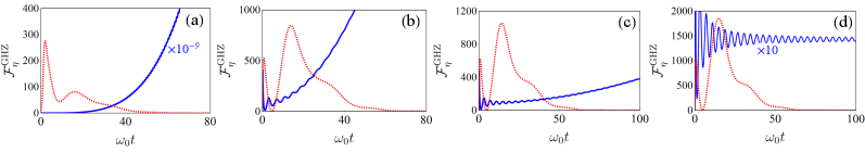
In the main text, we show the bound-state-favored quantum sensing of the reservoir in the large- limit. It is noted that the constructive role of the bound state in enhancing the sensing sensitivity is also present in the small- limit. Taking as an example, we plot in Fig. 3 its evolution in different . In the absence of the bound state, tends to zero irrespective of the value of . In contrast, becomes larger and larger with time in the small case when the bound state is formed. As analyzed in the last section, such persistent increasing QFI is contributed from in Eq. (A10). With the increasing of , the QFI from becomes smaller and smaller and tends to zero in the large- limit. Therefore, in this limit contains only the contribution from , which is a constant [see Eq. (A14)]. The numerical results in Fig. 3 are in good agreement with our above analytical solution, which validates our conclusion.
References
- Degen et al. (2017) C. L. Degen, F. Reinhard, and P. Cappellaro, “Quantum sensing,” Rev. Mod. Phys. 89, 035002 (2017).
- Caves (1981) Carlton M. Caves, “Quantum-mechanical noise in an interferometer,” Phys. Rev. D 23, 1693–1708 (1981).
- Pezzè et al. (2018) Luca Pezzè, Augusto Smerzi, Markus K. Oberthaler, Roman Schmied, and Philipp Treutlein, “Quantum metrology with nonclassical states of atomic ensembles,” Rev. Mod. Phys. 90, 035005 (2018).
- Zhang et al. (2018) Junhua Zhang, Mark Um, Dingshun Lv, Jing-Ning Zhang, Lu-Ming Duan, and Kihwan Kim, “NOON states of nine quantized vibrations in two radial modes of a trapped ion,” Phys. Rev. Lett. 121, 160502 (2018).
- Nagata et al. (2007) Tomohisa Nagata, Ryo Okamoto, Jeremy L. O’Brien, Keiji Sasaki, and Shigeki Takeuchi, “Beating the standard quantum limit with four-entangled photons,” Science 316, 726–729 (2007).
- Evrard et al. (2019) Alexandre Evrard, Vasiliy Makhalov, Thomas Chalopin, Leonid A. Sidorenkov, Jean Dalibard, Raphael Lopes, and Sylvain Nascimbene, “Enhanced magnetic sensitivity with non-gaussian quantum fluctuations,” Phys. Rev. Lett. 122, 173601 (2019).
- Haine and Hope (2020) Simon A. Haine and Joseph J. Hope, “Machine-designed sensor to make optimal use of entanglement-generating dynamics for quantum sensing,” Phys. Rev. Lett. 124, 060402 (2020).
- Muessel et al. (2014) W. Muessel, H. Strobel, D. Linnemann, D. B. Hume, and M. K. Oberthaler, “Scalable spin squeezing for quantum-enhanced magnetometry with Bose-Einstein condensates,” Phys. Rev. Lett. 113, 103004 (2014).
- Nolan et al. (2017) Samuel P. Nolan, Stuart S. Szigeti, and Simon A. Haine, “Optimal and robust quantum metrology using interaction-based readouts,” Phys. Rev. Lett. 119, 193601 (2017).
- Tse et al. (2019) M. Tse, Haocun Yu, N. Kijbunchoo, A. Fernandez-Galiana, P. Dupej, L. Barsotti, C. D. Blair, D. D. Brown, S. E. Dwyer, A. Effler, et al., “Quantum-enhanced advanced LIGO detectors in the era of gravitational-wave astronomy,” Phys. Rev. Lett. 123, 231107 (2019).
- Acernese et al. (2019) F. Acernese, M. Agathos, L. Aiello, A. Allocca, A. Amato, S. Ansoldi, S. Antier, M. Arène, N. Arnaud, S. Ascenzi, et al. (Virgo Collaboration), “Increasing the astrophysical reach of the advanced virgo detector via the application of squeezed vacuum states of light,” Phys. Rev. Lett. 123, 231108 (2019).
- Maccone and Ren (2020) Lorenzo Maccone and Changliang Ren, “Quantum radar,” Phys. Rev. Lett. 124, 200503 (2020).
- Kessler et al. (2014) E. M. Kessler, P. Kómár, M. Bishof, L. Jiang, A. S. Sørensen, J. Ye, and M. D. Lukin, “Heisenberg-limited atom clocks based on entangled qubits,” Phys. Rev. Lett. 112, 190403 (2014).
- Mehlstäubler et al. (2018) Tanja E Mehlstäubler, Gesine Grosche, Christian Lisdat, Piet O Schmidt, and Heiner Denker, “Atomic clocks for geodesy,” Reports on Progress in Physics 81, 064401 (2018).
- Potts et al. (2019) Patrick P. Potts, Jonatan Bohr Brask, and Nicolas Brunner, “Fundamental limits on low-temperature quantum thermometry with finite resolution,” Quantum 3, 161 (2019).
- Bouton et al. (2020) Quentin Bouton, Jens Nettersheim, Daniel Adam, Felix Schmidt, Daniel Mayer, Tobias Lausch, Eberhard Tiemann, and Artur Widera, “Single-atom quantum probes for ultracold gases boosted by nonequilibrium spin dynamics,” Phys. Rev. X 10, 011018 (2020).
- Troiani and Paris (2018) Filippo Troiani and Matteo G. A. Paris, “Universal quantum magnetometry with spin states at equilibrium,” Phys. Rev. Lett. 120, 260503 (2018).
- Razzoli et al. (2019) Luca Razzoli, Luca Ghirardi, Ilaria Siloi, Paolo Bordone, and Matteo G. A. Paris, “Lattice quantum magnetometry,” Phys. Rev. A 99, 062330 (2019).
- Cavina et al. (2018) Vasco Cavina, Luca Mancino, Antonella De Pasquale, Ilaria Gianani, Marco Sbroscia, Robert I. Booth, Emanuele Roccia, Roberto Raimondi, Vittorio Giovannetti, and Marco Barbieri, “Bridging thermodynamics and metrology in nonequilibrium quantum thermometry,” Phys. Rev. A 98, 050101(R) (2018).
- Hovhannisyan and Correa (2018) Karen V. Hovhannisyan and Luis A. Correa, “Measuring the temperature of cold many-body quantum systems,” Phys. Rev. B 98, 045101 (2018).
- Huelga et al. (1997) S. F. Huelga, C. Macchiavello, T. Pellizzari, A. K. Ekert, M. B. Plenio, and J. I. Cirac, “Improvement of frequency standards with quantum entanglement,” Phys. Rev. Lett. 79, 3865–3868 (1997).
- Wang et al. (2019) W. Wang, Y. Wu, Y. Ma, W. Cai, L. Hu, X. Mu, Y. Xu, Zi-Jie Chen, H. Wang, Y. P. Song, H. Yuan, C.-L. Zou, L.-M. Duan, and L. Sun, “Heisenberg-limited single-mode quantum metrology in a superconducting circuit,” Nature Communications 10, 4382 (2019).
- Chabuda et al. (2020) Krzysztof Chabuda, Jacek Dziarmaga, Tobias J. Osborne, and Rafal Demkowicz-Dobrzanski, “Tensor-network approach for quantum metrology in many-body quantum systems,” Nature Communications 11, 250 (2020).
- Gessner et al. (2019) Manuel Gessner, Augusto Smerzi, and Luca Pezzè, “Metrological nonlinear squeezing parameter,” Phys. Rev. Lett. 122, 090503 (2019).
- Gatto et al. (2019) Dario Gatto, Paolo Facchi, Frank A. Narducci, and Vincenzo Tamma, “Distributed quantum metrology with a single squeezed-vacuum source,” Phys. Rev. Research 1, 032024(R) (2019).
- Yu et al. (2020) Juan Yu, Yue Qin, Jinliang Qin, Hong Wang, Zhihui Yan, Xiaojun Jia, and Kunchi Peng, “Quantum enhanced optical phase estimation with a squeezed thermal state,” Phys. Rev. Applied 13, 024037 (2020).
- Zhuang and Zhang (2019) Quntao Zhuang and Zheshen Zhang, “Physical-layer supervised learning assisted by an entangled sensor network,” Phys. Rev. X 9, 041023 (2019).
- Kura and Ueda (2020) Naoto Kura and Masahito Ueda, “Standard quantum limit and Heisenberg limit in function estimation,” Phys. Rev. Lett. 124, 010507 (2020).
- Che et al. (2019) Yanming Che, Jing Liu, Xiao-Ming Lu, and Xiaoguang Wang, “Multiqubit matter-wave interferometry under decoherence and the Heisenberg scaling recovery,” Phys. Rev. A 99, 033807 (2019).
- Chen et al. (2020) Yu-Qin Chen, Kai-Li Ma, Yi-Cong Zheng, Jonathan Allcock, Shengyu Zhang, and Chang-Yu Hsieh, “Non-Markovian noise characterization with the transfer tensor method,” Phys. Rev. Applied 13, 034045 (2020).
- Goldwater et al. (2019) Daniel Goldwater, P. F. Barker, Angelo Bassi, and Sandro Donadi, “Quantum spectrometry for arbitrary noise,” Phys. Rev. Lett. 123, 230801 (2019).
- Mascherpa et al. (2017) F. Mascherpa, A. Smirne, S. F. Huelga, and M. B. Plenio, “Open systems with error bounds: Spin-boson model with spectral density variations,” Phys. Rev. Lett. 118, 100401 (2017).
- Xu et al. (2019) Shuang Xu, H. Z. Shen, X. X. Yi, and W. Wang, “Readout of the spectral density of an environment from the dynamics of an open system,” Phys. Rev. A 100, 032108 (2019).
- Farfurnik and Bar-Gill (2020) D. Farfurnik and N. Bar-Gill, “Characterizing spin-bath parameters using conventional and time-asymmetric Hahn-echo sequences,” Phys. Rev. B 101, 104306 (2020).
- Benedetti et al. (2018) Claudia Benedetti, Fahimeh Salari Sehdaran, Mohammad H. Zandi, and Matteo G. A. Paris, “Quantum probes for the cutoff frequency of Ohmic environments,” Phys. Rev. A 97, 012126 (2018).
- Bina et al. (2018) Matteo Bina, Federico Grasselli, and Matteo G. A. Paris, “Continuous-variable quantum probes for structured environments,” Phys. Rev. A 97, 012125 (2018).
- Tamascelli et al. (2020) Dario Tamascelli, Claudia Benedetti, Heinz-Peter Breuer, and Matteo G A Paris, “Quantum probing beyond pure dephasing,” New Journal of Physics 22, 083027 (2020).
- Sehdaran et al. (2019a) Fahimeh Salari Sehdaran, Mohammad H. Zandi, and Alireza Bahrampour, “The effect of probe-ohmic environment coupling type and probe information flow on quantum probing of the cutoff frequency,” Physics Letters A 383, 126006 (2019a).
- Sehdaran et al. (2019b) Fahimeh Salari Sehdaran, Matteo Bina, Claudia Benedetti, and Matteo G. A. Paris, “Quantum probes for ohmic environments at thermal equilibrium,” Entropy 21, 486 (2019b).
- Li et al. (2018) Li Li, Michael J.W. Hall, and Howard M. Wiseman, “Concepts of quantum non-Markovianity: A hierarchy,” Physics Reports 759, 1 – 51 (2018).
- Breuer et al. (2016) Heinz-Peter Breuer, Elsi-Mari Laine, Jyrki Piilo, and Bassano Vacchini, “Colloquium: Non-Markovian dynamics in open quantum systems,” Rev. Mod. Phys. 88, 021002 (2016).
- de Vega and Alonso (2017) Inés de Vega and Daniel Alonso, “Dynamics of non-Markovian open quantum systems,” Rev. Mod. Phys. 89, 015001 (2017).
- Rivas et al. (2014) Ángel Rivas, Susana F Huelga, and Martin B Plenio, “Quantum non-Markovianity: characterization, quantification and detection,” Reports on Progress in Physics 77, 094001 (2014).
- Streltsov et al. (2017) Alexander Streltsov, Gerardo Adesso, and Martin B. Plenio, “Colloquium: Quantum coherence as a resource,” Rev. Mod. Phys. 89, 041003 (2017).
- Kofman and Kurizki (2001) A. G. Kofman and G. Kurizki, “Universal dynamical control of quantum mechanical decay: Modulation of the coupling to the continuum,” Phys. Rev. Lett. 87, 270405 (2001).
- Soare et al. (2014) A. Soare, H. Ball, D. Hayes, J. Sastrawan, M. C. Jarratt, J. J. McLoughlin, X. Zhen, T. J. Green, and M. J. Biercuk, “Experimental noise filtering by quantum control,” Nature Physics 10, 825–829 (2014).
- Liu et al. (2019) Jing Liu, Haidong Yuan, Xiao-Ming Lu, and Xiaoguang Wang, “Quantum Fisher information matrix and multiparameter estimation,” Journal of Physics A: Mathematical and Theoretical 53, 023001 (2019).
- Giovannetti et al. (2004) Vittorio Giovannetti, Seth Lloyd, and Lorenzo Maccone, “Quantum-enhanced measurements: Beating the standard quantum limit,” Science 306, 1330–1336 (2004).
- Giovannetti et al. (2006) Vittorio Giovannetti, Seth Lloyd, and Lorenzo Maccone, “Quantum metrology,” Phys. Rev. Lett. 96, 010401 (2006).
- Bollinger et al. (1996) J. J . Bollinger, Wayne M. Itano, D. J. Wineland, and D. J. Heinzen, “Optimal frequency measurements with maximally correlated states,” Phys. Rev. A 54, R4649–R4652 (1996).
- Daryanoosh et al. (2018) Shakib Daryanoosh, Sergei Slussarenko, Dominic W. Berry, Howard M. Wiseman, and Geoff J. Pryde, “Experimental optical phase measurement approaching the exact Heisenberg limit,” Nature Communications 9, 4606 (2018).
- Frérot and Roscilde (2018) Irénée Frérot and Tommaso Roscilde, “Quantum critical metrology,” Phys. Rev. Lett. 121, 020402 (2018).
- Rams et al. (2018) Marek M. Rams, Piotr Sierant, Omyoti Dutta, Paweł Horodecki, and Jakub Zakrzewski, “At the limits of criticality-based quantum metrology: Apparent super-Heisenberg scaling revisited,” Phys. Rev. X 8, 021022 (2018).
- Chen et al. (2018) Geng Chen, Nati Aharon, Yong-Nan Sun, Zi-Huai Zhang, Wen-Hao Zhang, De-Yong He, Jian-Shun Tang, Xiao-Ye Xu, Yaron Kedem, Chuan-Feng Li, and Guang-Can Guo, “Heisenberg-scaling measurement of the single-photon kerr non-linearity using mixed states,” Nature Communications 9, 93 (2018).
- Wang et al. (2017) Yuan-Sheng Wang, Chong Chen, and Jun-Hong An, “Quantum metrology in local dissipative environments,” New Journal of Physics 19, 113019 (2017).
- Leggett et al. (1987) A. J. Leggett, S. Chakravarty, A. T. Dorsey, Matthew P. A. Fisher, Anupam Garg, and W. Zwerger, “Dynamics of the dissipative two-state system,” Rev. Mod. Phys. 59, 1–85 (1987).
- Ma et al. (2011) Jian Ma, Yi-xiao Huang, Xiaoguang Wang, and C. P. Sun, “Quantum Fisher information of the greenberger-horne-zeilinger state in decoherence channels,” Phys. Rev. A 84, 022302 (2011).
- Tan et al. (2013) Qing-Shou Tan, Yixiao Huang, Xiaolei Yin, Le-Man Kuang, and Xiaoguang Wang, “Enhancement of parameter-estimation precision in noisy systems by dynamical decoupling pulses,” Phys. Rev. A 87, 032102 (2013).
- Yang et al. (2014) Chun-Jie Yang, Jun-Hong An, Hong-Gang Luo, Yading Li, and C. H. Oh, “Canonical versus noncanonical equilibration dynamics of open quantum systems,” Phys. Rev. E 90, 022122 (2014).
- Tong et al. (2010) Qing-Jun Tong, Jun-Hong An, Hong-Gang Luo, and C. H. Oh, “Mechanism of entanglement preservation,” Phys. Rev. A 81, 052330 (2010).
- Wu et al. (2021) Wei Wu, Si-Yuan Bai, and Jun-Hong An, “Non-Markovian sensing of a quantum reservoir,” Phys. Rev. A 103, L010601 (2021).
- Bai et al. (2019) Kai Bai, Zhen Peng, Hong-Gang Luo, and Jun-Hong An, “Retrieving ideal precision in noisy quantum optical metrology,” Phys. Rev. Lett. 123, 040402 (2019).
- Liu and Houck (2017) Yanbing Liu and Andrew A. Houck, “Quantum electrodynamics near a photonic bandgap,” Nature Physics 13, 48–52 (2017).
- Krinner et al. (2018) Ludwig Krinner, Michael Stewart, Arturo Pazmiño, Joonhyuk Kwon, and Dominik Schneble, “Spontaneous emission of matter waves from a tunable open quantum system,” Nature 559, 589–592 (2018).