Threshold-Based Fast Successive-Cancellation Decoding of Polar Codes

In this paper, blackboard letters, such as $\mathbb{X}$, denote a set and $\left|\mathbb{X}\right|$ denotes the number of elements in $\mathbb{X}$. Bold letters, such as $\boldsymbol{v}$, denote a row vector, $\boldsymbol{v}^{T}$ denotes the transpose of $\boldsymbol{v}$, and notation $v\left[i:j\right]$, $1\leq i<j$ represents a subvector $\left(v\left[i\right],v\left[i+1\right],\dots,v\left[j\right]\right)$. $\oplus$ is used as the bitwise XOR operation and $v\left[i:j\right]\oplus z=\left(v\left[i\right]\oplus z,v\left[i+1\right]\oplus z,\dots,v\left[j\right]\oplus z\right)$, $z\in\left\{0,1\right\}$. The Kronecker product of two matrices $\mathbf{F}$ and $\mathbf{G}$ is written as $\displaystyle\mathbf{F}\otimes\mathbf{G}$. ${\mathbf{F}}_{N}$ represents an $N\times N$ square matrix and $\mathbf{F}_{N}^{\otimes n}$ denotes the $n$-th Kronecker power of $\mathbf{F}_{N}$. Throughout this paper, $\ln(x)$ denotes the natural logarithm and $\log(x)$ indicates the base-$2$ logarithm of $x$, respectively.

A polar code with code length $N=2^{n}$ and information length $K$ is denoted by $\mathcal{P}\left(N,K\right)$ and has rate $R=K/N$. The encoding can be expressed as $\boldsymbol{x}=\boldsymbol{u}\mathbf{G}_{N}$, where $\boldsymbol{u}=\left(u\left[1\right],u\left[2\right],\ldots,u\left[{N}\right]\right)$ is the input bit sequence and $\boldsymbol{x}=\left(x\left[1\right],x\left[2\right],\ldots,x\left[{N}\right]\right)$ is the encoded bit sequence. $\mathbf{G}_{N}=\mathbf{R}_{N}\mathbf{F}_{2}^{\otimes n}$ is the generator matrix, where $\mathbf{R}_{N}$ is a bit-reversal permutation matrix and $\mathbf{F}_{2}=\left[\begin{smallmatrix}1&0\\ 1&1\end{smallmatrix}\right]$.

The input bit sequence $\boldsymbol{u}$ consists of $K$ information bits and $N-K$ frozen bits. The information bits form set $\mathbb{A}$, transmitting information bits, while the frozen bits form set $\mathbb{A}^{c}$, transmitting fixed bits known to the receiver. For symmetric channels, without loss of generality, all frozen bits are set to zero [1]. To distinguish between frozen and information bits, a vector of flags $\boldsymbol{d}=\left(d\left[1\right],d\left[2\right],\ldots,d\left[{N}\right]\right)$ is used where each flag $d\left[k\right]$ is assigned as

The codeword $\boldsymbol{x}$ is transmitted through a channel after modulation. In this paper, non-systematic polar codes and binary phase-shift keying (BPSK) modulation that maps $\left\{0,1\right\}$ to $\left\{+1,-1\right\}$ are considered. Transmission takes place over an additive white Gaussian noise (AWGN) channel.

SC decoding can be illustrated on the factor graph of polar codes as shown in Fig. 2. The factor graph consists of $n+1$ levels and, by grouping all the operations that can be performed in parallel, SC decoding can be represented as the traversal of a binary tree. This traversal is shown in Fig. 2, starting from the left side of the binary tree. At level $j$ of the SC decoding tree with $n+1$ levels, there are $2^{n-j}$ nodes ($0\leq j\leq n$), and the $i$-th node at level $j$ ($1\leq i\leq 2^{n-j}$) of the SC decoding tree is denoted as $\mathcal{N}_{j}^{i}$. The left and the right child nodes of $\mathcal{N}_{j}^{i}$ are $\mathcal{N}_{j-1}^{2i-1}$ and $\mathcal{N}_{j-1}^{2i}$, respectively, as illustrated in Fig. 2. For $\mathcal{N}_{j}^{i}$, $\alpha_{j}^{i}\left[k\right]$, $1\leq k\leq 2^{j}$, indicates the $k$-th input logarithmic likelihood ratio (LLR) value, and $\beta_{j}^{i}\left[k\right]$, $1\leq k\leq 2^{j}$, denotes the $k$-th output binary hard-valued message. For the AWGN channel, the received vector $\boldsymbol{y}=\left(y\left[1\right],y\left[2\right],\ldots,y\left[N\right]\right)$ from the channel can be used to calculate the channel LLR as $2\boldsymbol{y}/\sigma^{2}$, where $\sigma^{2}$ is the variance of the Gaussian noise. SC decoding starts by setting $\alpha_{n}^{1}\left[1:N\right]=2\boldsymbol{y}/\sigma^{2}$. A node will be activated once all its inputs are available. When LLR messages pass through a node in the factor graph which is indicated by the $\oplus$ sign, the $f$ function over the LLR domain is executed as

and when LLR messages pass through a node in the factor graph which is indicated by the $$=$$ sign, the $g$ function over the LLR domain is executed as

where

The $f$ function can be approximated as [34]

When the LLR value of the $k$-th bit at level zero $\alpha_{0}^{k},\;1\leq k\leq N$, is calculated, the estimation of $u\left[k\right]$, denoted as ${\hat{u}}\left[k\right]$, can be obtained as

The hard-valued messages are propagated back to the parent node as

After traversing all the nodes in the SC decoding tree, $\hat{\boldsymbol{u}}$ contains the decoding result. Thus the latency of SC decoding for a polar code of length $N$ in terms of the number of time steps can be represented by the number of nodes in the SC decoding tree as [1]

The SC decoding has strong data dependencies that limit the amount of parallelism that can be exploited within the algorithm because the estimation of each bit depends on the estimation of all previous bits. This leads to a large latency in the SC decoding algorithm. It was shown in [9] that for a node $\mathcal{N}_{j}^{i}$, $\beta_{j}^{i}\left[1:2^{j}\right]$ can be estimated without traversing the decoding tree as

where $\mathbb{C}_{j}^{i}$ is the set of all the codewords associated with node $\mathcal{N}_{j}^{i}$. Multibit decoding can be performed directly in an intermediate level instead of bit-by-bit sequential decoding at level $0$, in order to traverse fewer nodes in the SC decoding tree and consequently, to reduce the latency caused by data computation and exchange. However, the evaluation of (10) generally requires exhaustive search over all the codewords in the set $\mathbb{C}_{j}^{i}$ which is computationally intensive in practice. In [12], a fast SC (FSC) decoding algorithm was proposed which performs fast parallel decoding when specific special node types are encountered. The sequences of information and frozen bits of these node types have special bit-patterns. Therefore, they can be decoded more efficiently without the need for exhaustive search. Using the vector $\boldsymbol{d}$, the five special node types proposed in [12] are described as:

• •

  Rate-0 node: all bits are frozen bits, $\boldsymbol{d}=\left(0,0,...,0\right)$.

• •

  Rate-1 node: all bits are non-frozen bits, $\boldsymbol{d}=\left(1,1,...,1\right)$.

• •

  REP node: all bits are frozen bits except the last one, $\boldsymbol{d}=\left(0,...,0,1\right)$.

• •

  SPC node: all bits are non-frozen bits except the first one, $\boldsymbol{d}=\left(0,1,...,1\right)$.

• •

  ML node: a code of length $4$ with $\boldsymbol{d}=\left(0,1,0,1\right)$.

By merging the aforementioned special nodes, five additional nodes were proposed, namely, the REP-SPC node, which is a REP node followed by a SPC node; the P-01/P-0SPC node, which is generated by merging a Rate-0 node with a Rate-1/SPC node; and the P-R1/P-RSPC node, which is generated by merging a $g$ function branch operation in (5) with the following Rate-1/SPC node. In [19], five additional special node types and their corresponding fast decoders were introduced. This enhanced FSC decoding algorithm can achieve a lower decoding latency than FSC decoding. The five special node types are:

• •

  Type-I node: all bits are frozen bits except the last two, $\boldsymbol{d}=\left(0,...,0,1,1\right)$.

• •

  Type-II node: all bits are frozen bits except the last three, $\boldsymbol{d}=\left(0,...,0,1,1,1\right)$.

• •

  Type-III node: all bits are non-frozen bits except the first two, $\boldsymbol{d}=\left(0,0,1,...,1\right)$.

• •

  Type-IV node: all bits are non-frozen bits except the first three, $\boldsymbol{d}=\left(0,0,0,1,...,1\right)$.

• •

  Type-V node: all bits are frozen bits except the last three and the fifth to last, $\boldsymbol{d}=\left(0,...,0,1,0,1,1,1\right)$.

A generalized FSC (GFSC) decoding algorithm was proposed in [20] by introducing the G-PC node and the G-REP node (previously identified as Multiple-G0 nodes in [23]). The G-PC node is a node at level $j$ having all its descendants as Rate-1 nodes except the leftmost one at a certain level $r<j$, that is a Rate-0 node. The G-REP node is a node at level $j$ for which all its descendants are Rate-0 nodes, except the rightmost one at a certain level $r<j$, which is a generic node of rate $C$ (Rate-C).

In [18], in addition to the nodes in [12], three special node types are added: the REP1 node, with the REP node on the left and the Rate-1 node on the right; the 0REPSPC node, which is a concatenation of the Rate-0, REP, and SPC nodes; and the 001 node, whose left $3/4$ of bits are frozen bits and right $1/4$ of bits are unfrozen bits.

To further reduce the latency, the operation merging scenarios are generalized in [22] and [23] where, in addition to merging special nodes, branch operation ((4),(5) and (8)) merging is also considered. Consequently, REP-REPSPC, REP-Rate1, and Rate0-ML nodes are adopted as the merging of special nodes, and F-REP node is adopted as a node-branch merger, which is generated by performing an $f$ function operation followed by a REP node. The following branch operation mergers are further introduced:

• •

  $\text{F}^{\times 2}$: two consecutive $f$ function operations in (4).

• •

  $\text{G0}^{\times 2}$: two consecutive G0 operations, where G0 is the $g$ function in (5) assuming $u=0$.

• •

  C^×2, C^×3: up to three consecutive operations in (8).

• •

  C0^×2, C0^×3: up to three consecutive operations in (8), assuming the estimations from the left branch are all zeros.

• •

  G-F: $g$ function operation followed by an $f$ function operation.

• •

  F-G0: $f$ function operation followed by a G0 operation.

The key advantage of using specific parallel decoders for the aforementioned special nodes is that, since the SC decoding tree is not traversed when one of these nodes is encountered, significant latency saving can be achieved. For example, if $\mathcal{N}_{j}^{i}$ is a Rate-1 node, hard decision decoding can be used to immediately obtain the decoding result as

If $\mathcal{N}_{j}^{i}$ is a SPC node, hard decision based on (11) is first derived followed by the calculation of the parity of the output using modulo-2 addition. The index of the least reliable bit is found as

Finally, the bits in a SPC node are estimated as

This operation can be performed in a single time step [19]. Finally, if $\mathcal{N}_{j}^{i}$ is a G-PC node, the decoding can be viewed as a parallel decoding of several separate SPC nodes. The decoding of a G-PC node can generally be performed in one time step considering parallel SPC decoders [20].

All of the aforementioned fast SC decoding algorithms perform decoding at an intermediate level of the decoding tree in order to reduce the number of traversed nodes. A decoding algorithm that can decode a node at a higher level of the decoding tree generally results in more savings in terms of latency than one that decodes a node at a lower level of the decoding tree.

For a binary AWGN channel with standard deviation $\sigma_{n}$, it was shown in [35] that, considering all the previous bits are decoded correctly, the LLR value $a_{j}^{i}\left[k\right]$, $1\leq k\leq 2^{j}$, input into node $\mathcal{N}_{j}^{i}$ can be approximated as a Gaussian variable using a Gaussian approximation as

where $M_{j}^{i}\left[k\right]$ is the expectation of $\alpha_{j}^{i}\left[k\right]$ [36] such that

and $m_{j}^{i}$ can be calculated recursively offline assuming the all-zero codeword is transmitted as

where

It was shown in [32] that, when the magnitude of the LLR values at a certain node in the SC decoding tree is large enough, the node has enough reliability to perform hard decision directly at the node without tangibly altering the error-correction performance. To determine the reliability of the node, a threshold is defined in [32] as

where $c_{t}\geq 1$ is a constant that is selected empirically. The hard-decision estimate of the received LLR values is calculated using

The issue with the method in [32] is that the threshold defined in (18) contains complex calculations of complementary error functions $\mathrm{erfc}\left(\cdot\right)$, making the corresponding calculation inefficient. Moreover, the hard-decision threshold is calculated empirically rather than for a desired error-correction performance and the threshold comparison in (19) is performed every time a node with no specific structure is encountered in the SC decoding process.

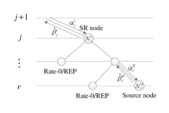
Let $\mathcal{N}_{j}^{i}$ be a node at level $j$ of the tree representation of SC decoding as shown in Fig. 2. An SR node is any node at stage $j$ whose descendants are all either Rate-0 or REP nodes, except the rightmost one at a certain stage $r$, $0\leq r\leq j$, that is a generic node of rate $C$. The structure of an SR node is depicted in Fig. 4. The rightmost node $\mathcal{N}_{r}^{i\times 2^{j-r}}$ at stage $r$ is denoted as the source node of the SR node $\mathcal{N}_{j}^{i}$. Let $E=i\times 2^{j-r}$ so the source node can be denoted as $\mathcal{N}_{r}^{E}$.

An SR node can be represented by three parameters as $\text{SR}(\boldsymbol{v},\text{SNT},r)$, where $r$ is the level of the SC decoding tree in which $\mathcal{N}_{r}^{E}$ is located, SNT is the source node type, and $\boldsymbol{v}=\left(v\left[{j}\right],v\left[{j-1}\right],\ldots,v\left[{r+1}\right]\right)$ is a vector of length $\left(j-r\right)$ such that for the left child node of the parent node of $\mathcal{N}_{r}^{E}$ at level $k$, $r<k\leq j$, $v\left[{k}\right]$ is calculated as

Note that when $r=j$, $\mathcal{N}_{j}^{i}$ is a source node and thus $\boldsymbol{v}$ is an empty vector denoted as $\boldsymbol{v}=\emptyset$.

To define the source node type, an extended class of G-PC (EG-PC) nodes is first introduced. The structure of the EG-PC node is depicted in Fig. 4. The EG-PC node is different from the G-PC node in its leftmost descendant node that can be either a Rate-0 or a REP node. The bits in an EG-PC node satisfy the following parity check constraint,

where $k\in\left\{1,\ldots,2^{r}\right\}$, and $z\in\left\{0,1\right\}$ is the parity. Unlike G-PC nodes whose parity is always even ($z=0$), the EG-PC node can have either even parity ($z=0$) or odd parity ($z=1$). The parity of the EG-PC node can be calculated as

where $\alpha_{k}=2\tanh^{-1}\left(\prod_{m=\left(k-1\right)2^{j-r}+1}^{k2^{j-r}}\tanh\left(\frac{\alpha_{j}^{i}\left[m\right]}{2}\right)\right)$. After computing $z$, Wagner decoders [37] can be used to decode the $2^{r}$ SPC codes with either even or odd parity constraints. A Wagner decoder performs hard decisions on the bits, and if the parity does not hold, it flips the bit with the lowest absolute LLR value.

SPC, Type-III, Type-IV, and G-PC nodes can be represented as special cases of EG-PC nodes. As a result, most of the common special nodes can be represented as SR nodes, as shown in Table I. Note that the node-branch mergers like P-RSPC and F-REP, and branch operation mergers such as $\text{F}^{\times 2}$, G‐F, $\text{G0}^{\times 2}$, F‐G0, do not fit into the category of SR nodes. It is worth mentioning that other parameter choices for SR nodes may lead to the discovery of more types of special nodes that can be decoded efficiently, but this exploration is beyond the scope of this work.

In this subsection, a set of sequences, called repetition sequences, is defined that can be used to calculate the output bit estimates of an SR node based on the output bit estimates of its source node. To derive the repetition sequences, $\boldsymbol{v}$ is used to generate all the possible sequences that have to be XORed with the output of the source node to generate the output bit estimates of the SR node. Let $\eta_{k}$ denote the rightmost bit value of the left child node of the parent node of $\mathcal{N}^{E}_{r}$ at level $k+1$. When $v[k+1]=0$, the left child node is a Rate-0 node so $\eta_{k}=0$. When $v[k+1]=1$, the left child node is a REP node, thus $\eta_{k}$ can take the value of either $0$ or $1$. The number of repetition sequences is dependent on the number of different values that $\eta_{k}$ can take. Let $W_{\boldsymbol{v}}$ denote the number of ‘$1$’s in $\boldsymbol{v}$. The number of all possible repetition sequences is thus $2^{W_{\boldsymbol{v}}}$. Let $\mathbb{S}=\{\boldsymbol{s}_{1},\ldots,\boldsymbol{s}_{2^{W_{\boldsymbol{v}}}}\}$ denote the set of all possible repetition sequences.

The output bits of SR node $\beta_{i}^{j}[1:2^{j}]$ have the property that their repetition sequence is repeated in blocks of length $2^{j-r}$. Let $\beta_{r}^{E}[1:2^{r}]$ denote the output bits of the source node of an SR node $\mathcal{N}_{j}^{i}$. The output bits for each block of length $2^{j-r}$ in $\mathcal{N}_{j}^{i}$ with respect to the output bits of its source node can be written as

where $k\in\left\{1,\dots,2^{r}\right\}$ and $\boldsymbol{s}_{l}=\{s_{l}[1],\ldots,s_{l}[2^{j-r}]\}$ is the $l$-th repetition sequence in $\mathbb{S}$. To obtain the repetition sequence $\boldsymbol{s}_{l}$ and with a slight abuse of terminology and notation for convenience, the Kronecker sum operator $\boxplus$ is used, which is equivalent to the Kronecker product operator, except that addition in GF($2$) is used instead of multiplication. For each set of values that $\eta_{k}$’s can take, $\boldsymbol{s}_{l}$ can be calculated as

For a polar code with a given $\boldsymbol{d}$, the locations of SR nodes in the decoding tree are fixed and can be determined off-line. Therefore, the repetition sequences in ${\mathbb{S}}$ of all of the SR nodes can be pre-computed and used in the course of decoding.

To decode SR nodes, the LLR values $\alpha_{r_{l}}^{E}[1:2^{r}]$ of the source node $\mathcal{N}_{r}^{E}$ are calculated based on the LLR values $\alpha_{j}^{i}[1:2^{j}]$ of the SR node $\mathcal{N}_{j}^{i}$ for every repetition sequence $\boldsymbol{s}_{l}$ as follows:

Using (23) and (25), (10) can be written as

Thus, the bit estimates of an SR node $\hat{\beta}_{j}^{i}\left[1:2^{j}\right]$ can be calculated by finding the bit estimates of its source node $\beta_{r}^{E}\left[1:2^{r}\right]$ using (26) and the repetition sequences as shown in (23).

The decoding algorithm of an SR node $\mathcal{N}_{j}^{i}$ is described in Algorithm 1. It first computes $\alpha_{r_{l}}^{E}$ for $l\in\left\{1,\dots,\left|{\mathbb{S}}\right|\right\}$ and generates $\left|{\mathbb{S}}\right|$ new paths by extending the decoding path at the $j-r$ rightmost bits corresponding to $\eta_{r},\eta_{r+1},\dots,\eta_{j-1}$. Note that the $l$-th path is generated when the repetition sequence is ${\boldsymbol{s}}_{l}$ and $\alpha_{r_{l}}^{E}$, $\widehat{\beta}_{r_{l}}^{E}$, and $\widehat{\beta}_{j_{l}}^{i}$ are its soft and hard messages. Then, the source node is decoded under the rule of the SC decoding. If the source node is a special node, a hard decision is made directly. Parity check and bit flipping will be performed further using Wagner decoder if the source node is an EG-PC node. Finally, the optimal decoding path index can be selected according to the comparison in (28) below and the decoding result is obtained using (23).

Based on Algorithm 1, the SR node-based fast SC (SRFSC) decoding algorithm is proposed. It follows the SC decoding algorithm schedule until an SR node is encountered where Algorithm 1 is executed. Note that the $\left|{\mathbb{S}}\right|$ paths can be processed simultaneously and the path selection operation in step 3 of Algorithm 1 can be performed in parallel with the decoding of the source node in step 2 and the following $g$ function operation. Once the selected index $\hat{l}$ is obtained, only the $l$-th decoding path corresponding to ${\boldsymbol{s}}_{l}$ is retained and the remaining paths are deleted.

In a binary AWGN channel, the LLR value $\alpha_{j}^{i}\left[k\right]$ of any node $\mathcal{N}_{j}^{i}$ can be approximated as a Gaussian variable as shown in Fig. 5. The red area in Fig. 5 represents the approximate probability of correct hard decision $\widetilde{P}_{c}$ and the blue area represents the approximate probability of incorrect hard decision $\widetilde{P}_{e}$ when $\beta_{j}^{i}\left[k\right]=0$ such that

where $Q\left(x\right)=\frac{1}{\sqrt{2\mathrm{\pi}}}\int_{x}^{\infty}e^{-\frac{t^{2}}{2}}dt$. The area between the two dashed lines represents the approximate probability that a hard decision is not performed.

To simplify the calculation of the threshold, we take a different approach than [32] by using the Gaussian distribution of $\alpha_{j}^{i}\left[k\right]$ and constraining the approximate probability of error when $\beta_{j}^{i}\left[k\right]=0$ to be

where $c$ (and thus $Q\left(c\right)$) is a positive constant, whose selection method will be given in Observation 1. This is equivalent to $T>-m_{j}^{i}+c\sqrt{2m_{j}^{i}}$. Therefore, the threshold is

where the absolute value ensures $T$ is positive for all values of $m_{j}^{i}>0$ with any $c>0$.

Under the Gaussian approximation in (14), for a node that undergoes hard decision in (19), the proposed threshold leads to a bounded probability of correct hard decision as shown in the following observation. Note that the analytical derivations are accurate under the assumption of Gaussian approximation.

Explanation: See Appendix B.

The proposed TA scheme performs hard decision on a node $\mathcal{N}_{j}^{i}$ only if (33) is satisfied. Furthermore, a hard decision is performed on a node if all of its input LLR values $\alpha_{j}^{i}\left[k\right]$ satisfy (19). Otherwise, standard SC decoding is applied on $\mathcal{N}_{j}^{i}$ to obtain the decoding result. Compared to the TA scheme in [32], the threshold values of both methods can be computed off-line. However, the proposed TA scheme in this paper has the following three advantages: 1) The proposed method can provide a higher latency reduction than the best case in [32] as shown in the simulation results; 2) The effect of the proposed threshold values on the error-correction performance is approximately predictable according to Observation 1; 3) According to (33), only a fraction of nodes undergo hard decision in the decoding process of the proposed TA scheme, which avoids unnecessary threshold comparisons. To speed up the decoding process, the proposed TA scheme is combined with SRFSC decoding that results in the TA-SRFSC decoding algorithm. In TA-SRFSC decoding, when one of the special nodes considered in SRFSC decoding is encountered, SRFSC decoding is performed and when a general node with no special structure is encountered, the proposed TA scheme is applied. The following observation provides an approximate upper bound on the BLER of the proposed TA-SRFSC decoding.

Explanation: See Appendix C.

Observation 2 provides a method to derive the threshold value for a desired upper bound of the BLER for TA-SRFSC decoding approximately. In fact, a large threshold value results in a better error-correction performance than a small threshold value at the cost of lower decoding speed. Therefore, a trade-off between the error-correction performance and the decoding speed can be achieved with the proposed TA-SRFSC decoding algorithm.

To mitigate the possible error-correction performance loss of the proposed TA-SRFSC decoding, a multi-stage decoding strategy is adopted in which a maximum of two decoding attempts is conducted. In the first decoding attempt, TA-SRFSC decoding is used. If this decoding fails and if there existed a node that underwent hard decision in this first decoding attempt, then a second decoding attempt using SRFSC decoding is conducted. To determine if the TA-SRFSC decoding failed, a cyclic redundancy check (CRC) is concatenated to the polar code and it is verified after the TA-SRFSC decoding. Additionally, the CRC is verified after the second decoding attempt by the SRFSC decoding to determine if the overall decoding process succeeded.

As shown in the next section, most of the received frames are decoded correctly by the proposed TA-SRFSC decoding in the first decoding attempt. As a result, the average decoding latency of the proposed multi-stage SRFSC decoding is very close to that of the TA-SRFSC decoding with CRC bits. However, the error-correction performance of the proposed multi-stage SRFSC decoding algorithm is slightly worse than that of SRFSC decoding due to the addition of CRC bits. As such, multi-stage SRFSC decoding trades off a slight degradation in error-correction performance to obtain a significant reduction in the average decoding latency. It is worth noting that, in order to improve the error-correction performance of the proposed scheme, the proposed multi-stage decoding strategy can be generalized to have more than two decoding attempts. In this scenario the first two attempts are the same as described above, i.e., TA-SRFSC decoding is used first followed by SRFSC decoding.¹¹1If the TA-SRFSC decoder does not satisfy the CRC, the SRFSC decoding either should start from the beginning or from the first node which underwent the hard decision. In this paper, the SRFSC decoder starts decoding from the first bit to avoid storing intermediate LLRs. The third and any subsequent attempts would use increasingly more powerful decoding techniques than the first two, such as SCL decoding.

In this case, the same assumptions as in [1, 19] are used and the decoding latency is measured in terms of the number of required time steps. More specifically: 1) there is no resource limitation so that all the parallelizable instructions are performed in one time step, 2) bit operations are carried out instantaneously, 3) addition/subtraction of real numbers and check-node operation consume one time step, and 4) Wagner decoding can be performed in one time step.

In this case, the decoding latency is measured in terms of the number of clock cycles in the actual hardware implementation. Contrary to Section V-A, a time step may take more than one clock cycle in a realistic hardware implementation. First, the idea of a semi-parallel decoder in [39] is adopted in which at most $P$ processing elements can run at the same time. Thus, parallel $f$ function or $g$ function operations on more than $P$ processing elements require more than one clock cycle. Second, the adder tree used for the calculation of LLR values in step 1 of Algorithm 1, and the compare-and-select (CS) tree used by the Wagner decoder to find the index of the least reliable input bit in step 2 of Algorithm 1, both require pipeline registers to reduce the critical path delay and improve the operating frequency and the overall throughput. The addition of these pipeline registers increases the number of decoding clock cycles. The exact number depends on the implementation and the given polar code.

References

- [1] E. Arıkan, “Channel polarization: A method for constructing capacity-achieving codes for symmetric binary-input memoryless channels,” IEEE Trans. Inf. Theory, vol. 55, no. 7, pp. 3051–3073, Jul. 2009.
- [2] 3GPP, “Final report of 3GPP TSG RAN WG1 #87 v1.0.0,” Reno, USA, Nov. 2016. [Online]. Available: http://www.3gpp.org/ftp/tsg_ran/WG1_RL1/TSGR1_87.
- [3] K. Niu, K. Chen, J. Lin, and Q. Zhang, “Polar codes: Primary concepts and practical decoding algorithms,” IEEE Commun. Mag., vol. 52, no. 7, pp. 192–203, 2014.
- [4] C. Zhang, B. Yuan, and K. K. Parhi, “Reduced-latency SC polar decoder architectures,” in Proc. IEEE Int. Conf. Commun. (ICC), Jun. 2012, pp. 3471–3475.
- [5] B. Yuan and K. K. Parhi, “Low-latency successive-cancellation polar decoder architectures using 2-bit decoding,” IEEE Trans. Circ. Syst. I: Regul., vol. 61, no. 4, pp. 1241–1254, April. 2014.
- [6] A. Mishra, A. J. Raymond, L. G. Amaru, G. Sarkis, C. Leroux, P. Meinerzhagen, A. Burg, and W. J. Gross, “A successive cancellation decoder ASIC for a 1024-bit polar code in 180nm cmos,” in Proc. Asian Solid-State Circuits Conf., Nov. 2012, pp. 205–208.
- [7] B. Yuan and K. K. Parhi, “Reduced-latency LLR-based SC list decoder for polar codes,” in Proc. 25th Ed. Great Lakes Symp. VLSI, May. 2015, pp. 107–110.
- [8] ——, “Low-latency successive-cancellation list decoders for polar codes with multibit decision,” IEEE Trans. VLSI Syst., vol. 23, no. 10, pp. 2268–2280, Oct. 2015.
- [9] G. Sarkis and W. J. Gross, “Increasing the throughput of polar decoders,” IEEE Commun. Lett., vol. 17, no. 4, pp. 725–728, Apr. 2013.
- [10] C. Husmann, P. C. Nikolaou, and K. Nikitopoulos, “Reduced latency ML polar decoding via multiple sphere-decoding tree searches,” IEEE Trans. Veh. Technol., vol. 67, no. 2, pp. 1835–1839, Feb. 2017.
- [11] A. Alamdar-Yazdi and F. R. Kschischang, “A simplified successive-cancellation decoder for polar codes,” IEEE Commun. Lett., vol. 15, no. 12, pp. 1378–1380, Dec. 2011.
- [12] G. Sarkis, P. Giard, A. Vardy, C. Thibeault, and W. J. Gross, “Fast polar decoders: Algorithm and implementation,” IEEE J. Sel. Areas Commun., vol. 32, no. 5, pp. 946–957, May. 2014.
- [13] P. Giard, G. Sarkis, C. Thibeault, and W. J. Gross, “Multi-mode unrolled architectures for polar decoders,” IEEE Trans. Circ. Syst. I: Regul., vol. 63, no. 9, pp. 1443–1453, Sep. 2016.
- [14] Z. Huang, C. Diao, and M. Chen, “Latency reduced method for modified successive cancellation decoding of polar codes,” Electron. Lett., vol. 48, no. 23, pp. 1505–1506, Nov. 2012.
- [15] A. Balatsoukas-Stimming, G. Karakonstantis, and A. Burg, “Enabling complexity-performance trade-offs for successive cancellation decoding of polar codes,” in Proc. IEEE Int. Symp. Inf. Theory Process. (ISIT), Jun. 2014, pp. 2977–2981.
- [16] L. Zhang, Z. Zhang, X. Wang, C. Zhong, and L. Ping, “Simplified successive-cancellation decoding using information set reselection for polar codes with arbitrary blocklength,” IET Commun., vol. 9, no. 11, pp. 1380–1387, Jul. 2015.
- [17] P. Giard, G. Sarkis, C. Thibeault, and W. J. Gross, “A 638 Mbps low-complexity rate 1/2 polar decoder on FPGAs,” in Proc. IEEE Int. Workshop Signal Process. Syst. (SiPS), Oct. 2015, pp. 1–6.
- [18] P. Giard, A. Balatsoukas-Stimming, G. Sarkis, C. Thibeault, and W. J. Gross, “Fast low-complexity decoders for low-rate polar codes,” J Sign Process Syst, vol. 90, no. 5, pp. 675–685, May. 2018.
- [19] M. Hanif and M. Ardakani, “Fast successive-cancellation decoding of polar codes: identification and decoding of new nodes,” IEEE Commun. Lett., vol. 21, no. 11, pp. 2360–2363, Nov. 2017.
- [20] C. Condo, V. Bioglio, and I. Land, “Generalized fast decoding of polar codes,” in Proc. IEEE Global Commun. Conf. (GLOBECOM), Dec. 2018, pp. 1–6.
- [21] H. Gamage, V. Ranasinghe, N. Rajatheva, and M. Latva-aho, “Low latency decoder for short blocklength polar codes,” arXiv preprint arXiv:1911.03201, 2019.
- [22] F. Ercan, C. Condo, and W. J. Gross, “Reduced-memory high-throughput Fast-SSC polar code decoder architecture,” in Proc. IEEE Int. Workshop Signal Process. Syst. (SiPS), Oct. 2017, pp. 1–6.
- [23] F. Ercan, T. Tonnellier, C. Condo, and W. J. Gross, “Operation merging for hardware implementations of fast polar decoders,” J Sign Process Syst, vol. 91, no. 9, pp. 995–1007, Sep. 2019.
- [24] P. Giard and A. Burg, “Fast-SSC-flip decoding of polar codes,” in Proc. IEEE Wireless Commun. Netw. Conf. Workshops (WCNCW), Apr. 2018, pp. 73–77.
- [25] F. Ercan, T. Tonnellier, and W. J. Gross, “Energy-efficient hardware architectures for fast polar decoders,” IEEE Trans. Circ. Syst. I: Regul., vol. 67, no. 1, pp. 322–335, Jan. 2020.
- [26] I. Tal and A. Vardy, “List decoding of polar codes,” IEEE Trans. Inf. Theory, vol. 61, no. 5, pp. 2213–2226, May. 2015.
- [27] G. Sarkis, P. Giard, A. Vardy, C. Thibeault, and W. J. Gross, “Fast list decoders for polar codes,” IEEE J. Sel. Areas Commun., vol. 34, no. 2, pp. 318–328, Feb. 2016.
- [28] S. A. Hashemi, C. Condo, and W. J. Gross, “A fast polar code list decoder architecture based on sphere decoding,” IEEE Trans. Circ. Syst. I: Regul., vol. 63, no. 12, pp. 2368–2380, Dec. 2016.
- [29] S. A. Hashemi, C. Condo, and W. J. Gross, “Fast and flexible successive-cancellation list decoders for polar codes,” IEEE Trans. Signal Process., vol. 65, no. 21, pp. 5756–5769, Nov. 2017.
- [30] S. A. Hashemi, C. Condo, M. Mondelli, and W. J. Gross, “Rate-flexible fast polar decoders,” IEEE Trans. Signal Process., vol. 67, no. 22, pp. 5689–5701, Nov. 2019.
- [31] M. H. Ardakani, M. Hanif, M. Ardakani, and C. Tellambura, “Fast successive-cancellation-based decoders of polar codes,” IEEE Trans. Commun., vol. 67, no. 7, pp. 4562–4574, Jul. 2019.
- [32] S. Li, Y. Deng, L. Lu, J. Liu, and T. Huang, “A low-latency simplified successive cancellation decoder for polar codes based on node error probability,” IEEE Commun. Lett., vol. 22, no. 12, pp. 2439–2442, Dec. 2018.
- [33] H. Sun, R. Liu, and C. Gao, “A simplified decoding method of polar codes based on hypothesis testing,” IEEE Commun. Lett., pp. 1–1, Jan. 2020.
- [34] C. Leroux, I. Tal, A. Vardy, and W. J. Gross, “Hardware architectures for successive cancellation decoding of polar codes,” in Proc. IEEE Int. Conf. Acoust., Speech Signal Process., May. 2011, pp. 1665–1668.
- [35] P. Trifonov, “Efficient design and decoding of polar codes,” IEEE Trans. Commun., vol. 60, no. 11, pp. 3221–3227, Nov. 2012.
- [36] Z. Zhang and L. Zhang, “A split-reduced successive cancellation list decoder for polar codes,” IEEE J. Sel. Areas Commun., vol. 34, no. 2, pp. 292–302, Feb. 2016.
- [37] R. Silverman and M. Balser, “Coding for constant-data-rate systems,” Trans. IRE Prof. Group Inf. Theory, vol. 4, no. 4, pp. 50–63, Sep. 1954.
- [38] M. El-Khamy, J. Lee, and I. Kang, “Detection analysis of CRC-assisted decoding,” IEEE Commun. Lett., vol. 19, no. 3, pp. 483–486, Mar. 2015.
- [39] C. Leroux, A. J. Raymond, G. Sarkis, and W. J. Gross, “A semi-parallel successive-cancellation decoder for polar codes,” IEEE Trans. Signal Process., vol. 61, no. 2, pp. 289–299, Jan. 2013.
- [40] 3GPP, “3GPP TS RAN 38.212 v1.2.1,” Dec. 2017. [Online]. Available: http://www.3gpp.org/ftp/Specs/archive/38_series/38.212/38212-f30.zip.
- [41] H. Zheng, A. Balatsoukas-Stimming, Z. Cao, and A. M. J. Koonen, “Implementation of a high-throughput Fast-SSC polar decoder with sequence repetition node,” arXiv:2007.11394, in IEEE Int. Workshop Signal Process. Syst. (SIPS), Oct. 2020.