11email: [email protected] 22institutetext: Astronomical Observatory, University of Warsaw, Al. Ujazdowskie 4, 00-478 Warszawa, Poland 33institutetext: Korea Astronomy and Space Science Institute, Daejon 34055, Republic of Korea 44institutetext: Dipartimento di Fisica “E. R. Caianiello”, Università di Salerno, Via Giovanni Paolo II, I-84084 Fisciano (SA), Italy 55institutetext: Istituto Nazionale di Fisica Nucleare, Sezione di Napoli, Via Cintia, I-80126 Napoli, Italy 66institutetext: University of Canterbury, Department of Physics and Astronomy, Private Bag 4800, Christchurch 8020, New Zealand 77institutetext: Korea University of Science and Technology, 217 Gajeong-ro, Yuseong-gu, Daejeon, 34113, Republic of Korea 88institutetext: Max Planck Institute for Astronomy, Königstuhl 17, D-69117 Heidelberg, Germany 99institutetext: Department of Astronomy, The Ohio State University, 140 W. 18th Ave., Columbus, OH 43210, USA 1010institutetext: Department of Particle Physics and Astrophysics, Weizmann Institute of Science, Rehovot 76100, Israel 1111institutetext: Center for Astrophysics Harvard & Smithsonian 60 Garden St., Cambridge, MA 02138, USA 1212institutetext: Department of Astronomy, Tsinghua University, Beijing 100084, China 1313institutetext: School of Space Research, Kyung Hee University, Yongin, Kyeonggi 17104, Republic of Korea 1414institutetext: Division of Physics, Mathematics, and Astronomy, California Institute of Technology, Pasadena, CA 91125, USA 1515institutetext: Department of Physics, University of Warwick, Gibbet Hill Road, Coventry, CV4 7AL, UK
Three faint-source microlensing planets detected via resonant-caustic channel
Abstract
Aims. We conducted a project of reinvestigating the 2017–2019 microlensing data collected by the high-cadence surveys with the aim of finding planets that were missed due to the deviations of planetary signals from the typical form of short-term anomalies.
Methods. The project led us to find three planets including KMT-2017-BLG-2509Lb, OGLE-2017-BLG-1099Lb, and OGLE-2019-BLG-0299Lb. The lensing light curves of the events have a common characteristic that the planetary signals were produced by the crossings of faint source stars over the resonant caustics formed by giant planets located near the Einstein rings of host stars.
Results. For all planetary events, the lensing solutions are uniquely determined without any degeneracy. It is estimated that the host masses are in the range of , which corresponds to early M to late K dwarfs, and thus the host stars are less massive than the sun. On the other hand, the planets, with masses in the range of , are heavier than the heaviest planet of the solar system, that is, Jupiter. The planets in all systems lie beyond the snow lines of the hosts, and thus the discovered planetary systems, together with many other microlensing planetary systems, support that massive gas-giant planets are commonplace around low-mass stars. We discuss the role of late-time high-resolution imaging in clarifying resonant-image lenses with very faint sources.
Key Words.:
gravitational microlensing – planets and satellites: detection| Event | (RA,DEC) | Alert date | ||
|---|---|---|---|---|
| KMT-2017-BLG-2509 | (17:42:21.57, -26:19:01.74) | postseason | 19.96 | |
| OGLE-2017-BLG-1099/ | (17:35:51.42, -29:35:09.10) | 2017-06-13/ | 20.61 | |
| KMT-2017-BLG-2336 | postseason | |||
| OGLE-2019-BLG-0299/ | (17:46:43.07,-23:35:03.52) | 2019-03-16/ | 20.04 | |
| KMT-2019-BLG-2735 | postseason |
| Event | Data sets | Field | Cadence |
|---|---|---|---|
| KMT-2017-BLG-2509 | KMTA, KMTC, KMTS | KMT18 | 1 hr |
| OGLE-2017-BLG-1099 | OGLE, | BLG654.2 | 1/3–1 day |
| KMTA, KMTC, KMTS | KMT14 | 1 hr | |
| OGLE-2019-BLG-0299 | OGLE, | BLG632.10 | 1/3–1 day |
| KMTA, KMTC, KMTS | KMT20 | 2.5 hr |
1 Introduction
During the early phase of planetary microlensing experiments, for example, OGLE (Udalski et al., 1994), MACHO (Alcock et al., 1993), EROS (Aubourg et al., 1993) surveys, for which the annual detection rate of lensing events was several dozens, individual events could be thoroughly inspected to check the existence of planet-induced anomalies in the light curves of the lensing events. With the advent of high-cadence surveys, that is, MOA (Sumi et al., 2013), OGLE-IV (Udalski et al., 2015), KMTNet (Kim et al., 2016), the detection rate has soared to more than 3000 per year. With the greatly increased number of events together with the large quantity of data for each event, planetary signals for some events may escape detection.
Two projects have been carried out since 2020 with the aim of finding missed planets in the survey data collected in and before the 2019 season. One project has been conducted to find planet-induced anomalies via an automatized algorithm. Hwang et al. (2021) applied the automated AnomalyFinder software (Zang et al., 2021) to the 2018–2019 lensing light curves from the of sky covered by the six KMTNet prime fields with cadences . From this investigation, they reported 6 newly detected planets with mass ratios , including OGLE-2019-BLG-1053Lb, KMT-2019-BLG-0253Lb, OGLE-2018-BLG-0506Lb, OGLE-2018-BLG-0516Lb, OGLE-2019-BLG-1492Lb, and OGLE-2018-BLG-0977. The signals of these planets were not only very short but also weak, and thus they had not been noticed from visual inspections. A more extensive searches for missing planetary signals are underway by applying the automated algorithm to all the lensing light curves detected by the KMTNet survey (Y. K. Jung et al. 2021, in preparation).
The other project has been conducted by visually inspecting the previous survey data to find unnoticed planetary signals. This project led to the discoveries of 10 planets. The first planet was KMT-2018-BLG-0748Lb (Han et al., 2020b), for which the planetary signal had been missed due to the faintness of the source combined with relatively large finite-source effects. This discovery was followed by the detections of KMT-2016-BLG-2364Lb, KMT-2016-BLG-2397Lb, OGLE-2017-BLG-0604Lb, and OGLE-2017-BLG-1375Lb, for all of which the lensing events involved faint source stars (Han et al., 2021a), KMT-2019-BLG-1339Lb, for which the planetary signal was partially covered (Han et al., 2020a), KMT-2018-BLG-1976Lb, OGLE-2019-BLG-0954Lb, KMT-2018-BLG-1996Lb, for which the planetary signals were produced through a non-caustic-crossing channel, and thus weak (Han et al., 2021b), and KMT-2018-BLG-1025Lb, for which the planetary signal had been missed due to the low mass ratio of the planet ( or for two degenerate solutions) together with the non-caustic-crossing nature of its planetary signal (Han et al., 2021c). Visually inspecting missing planets can provide various types of planetary signals that are prone to being missed, and thus can help to develop a more complete algorithm for automatized planet detections.
In this paper, we report three additional planets with similar planetary signatures and event characteristics found from the (visual) inspection of the 2017–2019 season data collected by the OGLE and KMTNet surveys. The common feature of these planetary events is that the planetary signals were produced by the crossings of faint source stars over the resonant caustics formed by giant planets located near the Einstein rings of the lens systems. Detecting such planetary signals requires a visual inspection of lensing light curves, because the durations of the planet-induced anomalies comprise important portions of the event durations, making them difficult to be detected by an automatized system that is optimized to detecting very short-term anomalies. An example of such a planetary event is found in the case of OGLE-2016-BLG-0596 (Mróz et al., 2017).
For the presentation of the work, we organize the paper as follows. In Sect. 2, we mention the observations of the lensing events and the acquired data. In Sect. 3, we mention the characteristics of the anomalies in the lensing light curves of the events, and describe the detailed analyses conducted to explain the observed anomalies. In Sect. 4, we specify the source types of the events, and constrain the angular Einstein radii. In Sect. 5, we determine the physical parameters of the planetary systems using the observables of the events. In Sect. 6, we discuss the role of high-resolution follow-up observations for faint-source planetary events with resonant caustic features in clarifying the nature of the lens system. A summary of the results and conclusion are presented in Sect. 7.
2 Observations and data
The newly reported three planetary lensing events are KMT-2017-BLG-2509, OGLE-2017-BLG-1099/KMT-2017-BLG-2336, and OGLE-2019-BLG-0299/KMT-2019-BLG-2735. The first event was detected solely by the KMTNet survey, and the latter two events were detected by both the OGLE and KMTNet surveys. Hereafter, we designate the events by the identification numbers of the surveys that first found the lensing events. In Table 1, we list the equatorial and galactic coordinates of the source stars, alert dates, and -band baseline magnitudes, , of the individual events. The notation “postseason” indicates that the event was detected from the postseason inspection of the data.
After one year test observations in the 2015 season, the KMTNet group has carried out a lensing survey toward the Galactic bulge field since 2016 with the use of three identical 1.6 m telescopes that are distributed in the three continents of the Southern Hemisphere, at the Siding Spring Observatory in Australia, the Cerro Tololo Interamerican Observatory in Chile, and the South African Astronomical Observatory in South Africa. We designate the individual telescopes as KMTA, KMTC, and KMTS, respectively. The camera mounted on each telescope has a 4 deg2 field of view. The OGLE team has conducted a lensing survey since its commencement of the first phase experiment in 1992 (Udalski et al., 1994), and now the survey is in the fourth phase (OGLE-IV) with the use of an upgraded camera yielding a 1.4 deg2 field of view (Udalski et al., 2015). The OGLE telescope with an aperture of 1.3 m is located at the Las Campanas Observatory in Chile. For both surveys, images of the events were obtained mainly in the band, and a fraction of -band images were acquired for the source color measurements. In Table 2, we list the data sets used in the analysis, the fields of the individual surveys, and the cadence of observations. We note that the KMTNet cadences of the events, ranging 1.0–2.5 hr, are substantially lower than the cadence of the prime fields, 15 min, and this partially contributed to the difficulty of identifying the planetary nature of the events.
| Event | Data set | (mag) | ||
| KMT-2017-BLG-2509 | KMTA | 1.054 | 0.020 | 200 |
| KMTC | 1.330 | 0.020 | 489 | |
| KMTS | 1.192 | 0.020 | 430 | |
| OGLE-2017-BLG-1099 | OGLE | 1.179 | 0.010 | 366 |
| KMTA | 1.149 | 0.020 | 139 | |
| KMTC | 1.054 | 0.010 | 183 | |
| KMTS | 1.025 | 0.030 | 225 | |
| OGLE-2019-BLG-0299 | OGLE | 1.265 | 0.010 | 249 |
| KMTA | 1.195 | 0.040 | 53 | |
| KMTC | 1.545 | 0.020 | 395 | |
| KMTS | 1.179 | 0.020 | 354 |

The data used in the analyses were reduced using the photometry pipelines of the individual survey groups. These pipelines, developed by Albrow et al. (2009) for KMTNet and by Woźniak (2000) for OGLE, utilize the difference imaging technique (Tomaney & Crotts, 1996; Alard & Lupton, 1998), which is optimized for the photometry of stars in very dense star fields. A subset of the KMTC data were additionally processed using the pyDIA photometry code (Albrow, 2017) to construct color-magnitude diagrams (CMD) of stars around the source stars and to specify the source types. See Sect. 4 for details. For the data used in the analyses, we readjusted the error bars of the photometric data by following the prescription depicted in Yee et al. (2012). Here denotes the error bar from the pipelines, is a factor used to make the scatter of data consistent with error bars, and is a scaling factor used to make the per degree of freedom for each data equal to unity. In Table 3, we list the error-bar readjustment factors and the number of data, , of the individual data sets.
3 Analysis
In this section, we present the detailed analyses of the individual lensing events. The light curves of all events exhibit anomaly features that include caustic crossings, and thus we model the light curves under a binary-lens and single-source (2L1S) interpretation.

The modeling is done by searching for the set of the lensing parameters that best explain the observed data. The first three of these parameters describe the source–lens approach, including , which represent the time of the closest source approach to a reference position of the lens, the separation (normalized to the angular Einstein radius ) between the source and the lens reference position at , and the event time scale, respectively. For the reference position of the lens, we use the center of mass for a binary lens with a separation less than (close binary), and the effective position, defined by Di Stefano & Mao (1996) and An & Han (2002), for the lens with a separation greater than (wide binary). The next three parameters describe the lens binarity, and they denote the projected separation (normalized to ) and mass ratio between the lens components, and , and the angle between the source motion and the binary axis (source trajectory angle), respectively. The last parameter is , which is defined as the ratio of the angular source radius, , to , that is, (normalized source radius), and it is included to account for finite-source effects that affect the caustic-crossing parts of lensing light curves. We incorporate limb-darkening effects in the finite magnification computations by modeling the surface brightness variation of the source as , where is the limb-darkening coefficient, represents the angle between two lines extending from the source center: one to the observer and the other to the source surface. As will be discussed in Sect. 4, the source stars of all events have similar spectral types, early K-type main-sequence stars, and thus we adopt an -band limb-darkening coefficient of from Claret (2000), assuming that the effective temperature, surface gravity, and turbulence velocity are K, , and , respectively.
For a fraction of events with long time scales comprising an important protion of a year, lensing light curves may deviate from the form expected from a rectilinear lens-source motion. One cause for this deviation is the motion of an observer induced by the orbital motion of Earth (microlens-parallax effect: Gould, 1992), and the other is the orbital motion of the binary lens (lens-orbital effects: Dominik, 1998). It is expected that the signature of the microlens parallax, , will be small for OGLE-2017-BLG-1099 and OGLE-2019-BLG-0299 due to their short time scales, which are days and days, respectively, but the signature might not be small for KMT-2017-BLG-2509 due to its relatively long time scale of days. We check these higher-order effects and find that it is difficult to detect the higher-order signatures for any of the events, mainly because the photometric quality is not high enough to detect the subtle deviations induced by these higher-order effects. A microlens parallax can provide an important constraint on the physical lens parameters. As will be discussed in Sect. 5, the uncertainties of the physical lens parameters are large for all events due to the absence of the constraint.

| Parameter | KMT-2017-BLG-2509 | OGLE-2017-BLG-1099 | OGLE-2019-BLG-0299 |
|---|---|---|---|
| (HJD′) | |||
| (days) | |||
| (10-3) | |||
| (rad) | |||
| (10-3) | |||
The 2L1S modeling is carried out in two steps. In the first step, the binary lensing parameters and are searched for using a grid approach with different starting values of evenly distributed in the 0 – range with 21 grids, while the 5 non-grid lensing parameters, that is, , are found using a downhill approach based on the Markov Chain Monte Carlo (MCMC) algorithm. The ranges of the grid parameters are and , and they are divided into 70 grids. We then identify local solutions that appear in the map on the – parameter plane. In the second step, we refine the individual local solutions found in the first step by letting all parameters vary. Then the global solution is found by comparing values of the local solutions, if there is more than one. Figure 1 shows the maps on the – parameter plane obtained from the first-step modeling of the individual events. It shows that there exist a single local solution for all events.

3.1 KMT-2017-BLG-2509
Figure 2 shows the lensing light curve of KMT-2017-BLG-2509. It is characterized by two distinctive caustic features that appear at and in . For the first caustic feature, both the rising (covered by 4 KMTA data points) and falling sides (by a single KMTC point) were captured, while only the rising side was covered (by 5 KMTC points) for the second feature. See the zoom-in view of the anomaly region shown in Figure 3. The region between the two caustic features exhibits negative deviations from a single-lens single-source (1L1S) light curve. To be noted about the light curve is that the error bars of the data are substantial due to the faintness of the source, and the anomaly region occupies a large portion of the magnified region of the light curve. This made it difficult for the anomalies to be readily noticed as a planetary (rather than a stellar-binary) signal.222 The caustic morphology and mass ratio of KMT-2017-BLG-2509 is similar to those of MOA-2009-BLG-387 (Batista et al., 2011). When there were relatively few microlensing events being discovered, MOA-2009-BLG-387 was easily identified as a planet, while the planetary nature of KMT-2017-BLG-2509 had not been noticed until this paper. This indicates that more rigorous review of anomalies in the previous microlensing data is important for the accurate estimation of microlensing planet statistics.
The 2L1S modeling yields binary parameters of , indicating that the companion to the primary lens is a planetary-mass object lying near the Einstein ring of the primary. We find a unique solution without any degeneracy. For a lensing event produced by a binary lens with a small mass ratio, there often exists a pair of close () and wide () solutions arising from the similarity between the central caustics induced by the companions with and : the close–wide degeneracy (Griest & Safizadeh, 1998; Dominik, 1999). It is found that KMT-2017-BLG-2509 is not subject to this degeneracy because the light-curve morphology (two pairs of caustic crossings that flank a demagnified region) is strictly characteristic of an geometry. See Figure 4. The normalized source radius, , is measured by analyzing the caustic-crossing parts of the light curve.
The model curve of the 2L1S solution is drawn over the data points in Figures 2 and 3. In Table 4, we list the full lensing parameters of the model together with the flux parameters of the source, , and blend, , in which the flux is approximately scaled to that of , that is, . Figure 4 shows the configuration of the lens system corresponding to the solution. In the figure, the line with an arrow indicates the source motion, the red closed figure is the caustic, the blue dots, marked by and in the inset, denote the lens positions, and the dashed circle represents the Einstein ring. The planet is located close to the Einstein ring, and this results in a single, six-sided resonant caustic. The caustic appears as the merging of the single central caustic and the two sets of planetary caustics. The source crossed the tip of the lower planetary caustic at , and then crossed the slim bridge connecting the upper planetary caustic and the central caustic at . We mark the source positions corresponding to and by empty magenta dots. We note that the size of the dot is not scaled to the source size. The negative deviation region between and occurred when the source passed through the negative deviation region formed between the two planetary caustics.


3.2 OGLE-2017-BLG-1099
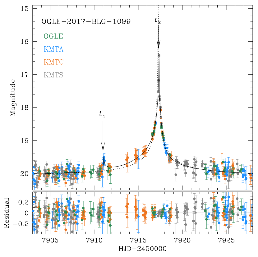
The lensing light curve of OGLE-2017-BLG-1099 is shown in Figure 5. The online data of the event posted on the alert web pages of the individual survey groups333http://ogle.astrouw.edu.pl/ogle4/ews/ews.html for the OGLE survey, and https://kmtnet.kasi.re.kr/ ulens/ for the KMTNet survey. did not show an obvious anomaly feature in the light curve. Nevertheless, the event was selected for a detailed analysis because it reached a very high magnification, , during which the chance of detecting a planet-induced anomaly was high (Griest & Safizadeh, 1998). Optimal light curve obtained by rereducing the data revealed that the light curve was anomalous. The anomaly is characterized first by the asymmetry of the light curve, and second by the caustic-involved feature at . See the zoom-in view of the region around presented in the right panel of Figure 6. It shows that the five KMTS data points exhibit the characteristic pattern of magnification variation occurring when a source exits a caustic. See Figure 1 of Gould & Andronov (1999).

The 2L1S modeling yields a unique solution with the binary parameters of , indicating that the companion is a planetary-mass object with a separation similar to . We note that the analysis of the event was done in the 2017 season and its planetary nature was realized by one of the coauthors (Y.-H. Ryu), but the result was not shared with the other coauthors. As a result, the analysis presented in this work is carried out independently, reaching at a result that is consistent with the previous one. The full lensing parameters are listed in Table 4, and the model curve is presented in Figures 5 and 6. Due to the proximity of the binary separation to unity, the binary lens pair forms a single resonant caustic. According to the model, the source entered the caustic at , and exited the caustic at . Due to the weakness of the caustic combined with the low photometric precision, the anomaly feature occurred at around the caustic entrance was difficult to be noticed in the preliminary modeling using the online data, but the rereduced data showed that the caustic was covered by four KMTA data points, although the uncertainties of the data points around the caustic exist were still large. See the zoom-in view around shown in the left panel of Figure 6. The coverage of both the caustic entrance and exit yields a normalized source radius of .
Figure 7 shows the configuration of the lens system. Like the case of KMT-2017-BLG-2509, the caustic appears as the merging of the planetary and central caustics. The source moved approximately in parallel with the binary axis (). It entered the caustic by passing the lower right side of the planetary caustic, generating a weak caustic spike at . Then, the source exited the caustic by passing the left side of the central caustic, and then passed the region close to the back-end cusp of the central caustic, and this produced the caustic feature at . See the zoom-in view of the central region presented in the left inset. The two empty magenta dots on the source trajectory of the main panel represent the source positions at and . We note that the size of these dots is arbitrarily set, but the source dot in the left inset is scaled to the source size.

3.3 OGLE-2019-BLG-0299
Figure 8 shows the light curve of OGLE-2019-BLG-0299. The anomalous nature of the light curve was known when the event was proceeding, and planetary-lensing models found with the use of the OGLE data were circulated to the microlensing community by C. Han and V. Bozza before the end of the event. The analysis in this work is done with the addition of the KMTNet data obtained from the optimized photometry of the event. The enlarged view of the light curve around the anomaly region is shown in Figure 9. The anomaly exhibits a very complex pattern, that is characterized by 6 peaks or bumps at , , , , , and .
A 2L1S modeling yields a unique solution with the binary parameters of . The binary separation is very close to unity, as in the cases of the two previous events. The mass ratio is about ten times the Jupiter/sun ratio of the solar system, but the mass of the companion is still in the planet-mass regime, considering that the measured event time scale, days, is not much longer than those of typical lensing events produced by low-mass stars. The full lensing parameters are presented in Table 4. Although all the major anomaly features were delineated, none of the caustics was resolved densely enough for the secure measurement of , and only the upper limit, , is constrained.

Figure 10 shows the lens system configuration of OGLE-2019-BLG-0299. According to the model, the source crossed the binary axis with a source trajectory angle of , and passed through the 6-fold resonant caustic four times at , , , and , where and ) are the two time pairs of caustic entrance and exit. These caustic crossings produced the spikes at the corresponding times, and the regions of the light curve between the individual caustic-crossing pairs exhibited characteristic U-shape trough patterns. The bump at was produced by the source approach close to the lower cusp of the caustic before the first caustic crossing at . The other bump at was produced when the source passed through the outer-caustic region near the left-side on-axis cusp of the caustic. The source positions corresponding to the 6 epochs of the anomaly are marked by empty magenta dots, of which size is not scaled, on the source trajectory.
| Quantity | KMT-2017-BLG-2509 | OGLE-2017-BLG-1099 | OGLE-2019-BLG-0299 |
|---|---|---|---|
| (as) | |||
| (mas) | |||
| (mas/yr) |
4 Source stars and Einstein radii
In this section, we estimate the angular Einstein radii of the events. The Einstein radius is determined by . The value is measured or constrained from the analysis of the caustic-crossing parts, which are affected by finite-source effects. With the measured , then it is required to estimate the angular source radius . The value of is deduced from the color and magnitude of the source.
In general, the source color is estimated by measuring the source magnitudes in two passbands, and bands in our case, by regressing the data of the individual passbands with the variation of the lensing magnification. The -band magnitudes are securely measured by this method for all events. However, the -band magnitudes are difficult to be measured by this method due to the large uncertainties of the data, making it difficult to securely estimate the source colors. We, therefore, estimate the source color using the Bennett et al. (2008) method, which utilizes the CMD constructed from the Hubble Space Telescope (HST) observations (Holtzman et al., 1998). In the first step of this method, the HST CMD is aligned with the CMD obtained from ground-based observations using the well defined centroid of the red giant clump (RGC). In the second step, the source position in the CMD is interpolated from the branch of main-sequence or giant stars on the HST CMD using the well measured -band magnitude difference between the RGC centroid and the source. In the final step, the source color and its uncertainty are estimated as the mean and standard deviation of stars located on the branch.
Figure 11 shows the source locations (black filled dots with error bars) with respect to the RGC centroids (red filled dot) in the combined CMD, in which the HST CMD is represented by brown dots and the CMD from the ground-based observations is represented by grey dots. In Table 5, we list the positions of the source, , and the RGC centroid, , measured on the instrumental CMD. Then, the reddening and extinction corrected (de-reddened) color and magnitude of the source, , are determined using the offsets from the RGC centroid, , together with the known de-reddened values of RGC, (Bensby et al., 2013; Nataf et al., 2013), by the relation
| (1) |
The values of , , for the individual events are listed in Table 5. We note that the de-reddened -band magnitudes of the RGC centroids, that is, , vary depending on the event, because we consider the varying distance depending on the source location using Table 1 of Nataf et al. (2013). The measured colors and magnitudes, which are in the ranges of and , respectively, indicate that the source stars of the events have similar spectral types of early K-type main sequence stars.

The measured color is then converted into color using the color-color relation of Bessell & Brett (1988), and then the source radius is deduced from the – relation of Kervella et al. (2004). With the measured source radius, then, the Einstein radius and the relative lens-source proper motion are estimated by the relations and , respectively. We list the estimated values of , , and in Table 5. We note that the lower limits and are presented for OGLE-2019-BLG-0299, because only the upper limit of is constrained for the event.
| Parameter | KMT-2017-BLG-2509 | OGLE-2017-BLG-1099 | OGLE-2019-BLG-0299 |
|---|---|---|---|
| () | |||
| () | |||
| (kpc) | |||
| (AU) |
5 Physical lens parameters
We estimate the physical lens parameters of the lens mass, , and distance, , by conducting a Bayesian analysis. The lensing observables that can be used to constrain and include , , and , where the first two observables are related to and by
| (2) |
and the additional measurement of would allow one to uniquely determine the lens parameters by
| (3) |
Here , , and denotes the distance to the source (Gould, 2000). The available observables vary depending on the events: and for KMT-2017-BLG-2509 and OGLE-2017-BLG-1099, and and the lower limit of for OGLE-2019-BLG-0299. The value of is not measured for any of the events.
In the first step of the Bayesian analysis, we produce artificial lensing events by conducting a Monte Carlo simulation. In the simulation, we use a prior Galactic model, which describes the physical and dynamical distributions and the mass function of Galactic objects. We adopt the Jung et al. (2021) Galactic model, in which the physical distribution of disk and bulge objects are described by the Robin et al. (2003) and Han & Gould (2003) models, respectively, the dynamical distributions of the disk and bulge objects are depicted by the Jung et al. (2021) and Han & Gould (1995) models, respectively, and the Jung et al. (2018) mass function model is commonly used for both populations. In the second step, we choose events with and values consistent with the measured observables, and construct the posterior distributions of and for these events. Then, the representative values of the lens parameters are determined as the median values of the posterior distributions, and the lower and upper limits are determined as 16% and 84% of the distributions, respectively.

In Figures 12 and 13 , we present the Bayesian posterior distributions of and , respectively. In Table 6, we list the estimated masses of the host, , and planet, , distance, and projected planet-host separation, . The projected separation is calculated by . It is estimated that the host masses are in the range of , which corresponds to early M to late K dwarfs, and thus the host stars are less massive than the sun. On the other hand, the planet masses, which are in the range of , are heavier than the mass of the heaviest planet of the solar system, that is, Jupiter. Considering that the snow line distance is AU, and is the separation in projection, the planets in all systems lie beyond the snow lines of the hosts. Therefore, the discovered planetary systems, together with many other microlensing planetary systems, support that massive gas-giant planets are commonplace around low-mass stars. See the distribution of exoplanets with respect to presented in Figure 6 of Gaudi (2012). The contributions to the posterior distribution by the disk and bulge lens populations are marked by blue and red curves, respectively. The disk/bulge contributions are 28%/72% for KMT-2017-BLG-2509, 33%/67% for OGLE-2017-BLG-1099, and 48%/52% for OGLE-2019-BLG-0299. The relatively low disk contribution for KMT-2017-BLG-2509 arises due to the constraint of the low relative lens-source proper motion, mas/yr, because low proper motion is difficult to produce for disk lenses.

6 High-resolution follow-up observation
In the general case of a lensing event, high-resolution observations using space-borne telescopes or ground-based adaptive optics instruments allow one to measure the lens flux and the lens-source separation. The lens flux allows one to estimate the lens mass , and the lens-source separation allows one to estimate the relative lens-source proper motion , which in turn constrains the Einstein radius by .
For faint-source planetary lensing events with resonant caustic features, high-resolution follow-up observations are especially important for clarifying the planetary lens systems. The size of a resonant planetary caustic scales to the planet/host mass ratio as , and thus the duration of the planetary anomaly is related to the event time scale by . For a given anomaly duration, then, the event time scale and the mass ratio are related by . For faint-source events, the very faint sources can make it difficult to precisely determine , and this leads to a large uncertainty of , because . Late time observations in two passbands can yield the source flux and color, and so -band source-flux estimate. The well estimated source flux can further constrain , and this leads to a tight constraint on the planet mass ratio. High-resolution image data could have resulted in best constraints if they had been acquired at the time of the event to provide a comparison. Unfortunately, no such images were taken because the planetary nature of the events were not known at the times of the event discoveries. However, post-event imaging can still help to constrain the physical parameters the lens systems.
7 Summary and conclusion
We reported three microlensing planets KMT-2017-BLG-2509Lb, OGLE-2017-BLG-1099Lb, and OGLE-2019-BLG-0299Lb that were found from the reinvestigation of the microlensing data collected by the KMTNet and OGLE surveys during the 2017–2019 seasons. For all of these lensing events, the planetary signals deviated from the typical form of short-term anomalies, because they were produced by the crossings of the source stars over the resonant caustics formed by the giant planets located at around the Einstein rings of host stars. The faintness of the source stars and the relatively low observational cadences also contributed to the difficulty of finding the planetary signals. Due to the resonant nature of the caustics, the lensing solutions were uniquely determined without any degeneracy. The estimated masses of the planet hosts are in the range of , which corresponds to early M to late K dwarfs, and thus the host stars are less massive than the sun. On the other hand, the planets, with masses in the range of , are heavier than Jupiter of the solar system. The planets in all systems lie beyond the snow lines of the hosts, and thus the discovered planetary systems support the conclusion that massive gas-giant planets are commonplace around low-mass stars.
Acknowledgements.
Work by C.H. was supported by the grants of National Research Foundation of Korea (2019R1A2C2085965 and 2020R1A4A2002885). This work was conducted during the research year of Chungbuk National University in 2021. This research has made use of the KMTNet system operated by the Korea Astronomy and Space Science Institute (KASI) and the data were obtained at three host sites of CTIO in Chile, SAAO in South Africa, and SSO in Australia. The OGLE project has received funding from the National Science Centre, Poland, grant MAESTRO 2014/14/A/ST9/00121 to AU.References
- Alard & Lupton (1998) Alard, C., & Lupton, R. H. 1998, ApJ, 503, 325
- Albrow (2017) Albrow, M. 2017, MichaelDAlbrow/pyDIA: Initial Release on Github,Version v1.0.0, Zenodo, doi:10.5281/zenodo.268049
- Albrow et al. (2009) Albrow, M., Horne, K., Bramich, D. M., et al. 2009, MNRAS, 397, 2099
- Alcock et al. (1993) Alcock, C., Akerlof, C. W., Allsman, R. A., et al. 1993, Nature, 365, 621
- An & Han (2002) An, J. H., & Han, C. 2002, ApJ, 573, 351
- Aubourg et al. (1993) Aubourg, E., Bareyre, P., Bréhin, S., et al. 1993, Nature, 365, 623
- Batista et al. (2011) Batista, V., Gould, A., Dieters, S., et al. 2011, A&A, 529, A102
- Bennett et al. (2008) Bennett, D. P., Bond, I. A., Udalski, A., et al. 2008, ApJ, 684, 663B
- Bensby et al. (2013) Bensby, T., Yee, J. C., Feltzing, S., et al. 2013, A&A, 549, 14
- Bessell & Brett (1988) Bessell, M. S., & Brett, J. M. 1988, PASP, 100, 1134
- Claret (2000) Claret, A. 2000, A&A, 363, 1081
- Di Stefano & Mao (1996) Di Stefano, R., & Mao, S. 1996, ApJ, 457, 93
- Dominik (1998) Dominik, M. 1998, A&A, 329, 361
- Dominik (1999) Dominik, M. 1999, A&A, 349, 108
- Gaudi (2012) Gaudi, B. S. 2012, ARA&A, 50, 411
- Gould (1992) Gould, A. 1992, ApJ, 392, 442
- Gould (2000) Gould, A. 2000, ApJ, 542, 785
- Gould & Andronov (1999) Gould, A., & Andronov, N. 1999, ApJ, 516, 236
- Griest & Safizadeh (1998) Griest, K., & Safizadeh, N. 1998, ApJ, 500, 37
- Han & Gould (1995) Han, C., & Gould, A. 1995, ApJ, 447, 53
- Han & Gould (2003) Han, C., & Gould, A. 2003, ApJ, 592, 172
- Han et al. (2020a) Han, C., Kim, D., Udalski, A., et al. 2020a, AJ, 160, 64
- Han et al. (2020b) Han, C., Shin, I.-G., Jung, Y. K., et al. 2020b, A&A, 641, A105
- Han et al. (2021a) Han, C., Udalski, A., Kim, D., et al. 2021a, A&A, 642, 110
- Han et al. (2021b) Han, C., Udalski, A., Kim, D., et al. 2021b, A&A, 650, A89
- Han et al. (2021c) Han, C., Udalski, A., Kim, D., et al. 2021c, A&A, 649, A90
- Holtzman et al. (1998) Holtzman, J. A., Watson, A. M., Baum, W. A., et al. 1998, AJ, 115, 1946
- Hwang et al. (2021) Hwang, W., Zang, W., Gould, A., et al. 2021, in preparation
- Jung et al. (2021) Jung, Y. K., Han, C., Udalski, A., et al. 2021, AJ, 161, 293
- Jung et al. (2018) Jung, Y. K., Udalski, A., Gould, A., et al. 2018, AJ, 155, 219
- Kervella et al. (2004) Kervella, P., Thévenin, F., Di Folco, E., & Ségransan, D. 2004, A&A, 426,29
- Kim et al. (2016) Kim, S.-L., Lee, C.-U., Park, B.-G., et al. 2016, JKAS, 49, 37
- Mróz et al. (2017) Mróz, P., Han, C., Udalski, A., et al. 2017, AJ, 153, 143
- Nataf et al. (2013) Nataf, D. M., Gould, A., Fouqué, P., et al. 2013, ApJ, 769, 88
- Robin et al. (2003) Robin, A. C., Reylé, C., Derriére, S., & Picaud, S. 2003, A&A, 409, 523
- Sumi et al. (2013) Sumi, T., Bennett, D. P., Bond, I. A., et al. 2013, ApJ, 778, 150
- Tomaney & Crotts (1996) Tomaney, A. B., & Crotts, A. P. S. 1996, AJ, 112, 2872
- Udalski et al. (1993) Udalski, A., Szymański, M., Kałużny, J., et al. 1993, Acta Astron., 43, 289
- Udalski et al. (1994) Udalski, A., Szymański, M., Kałużny, J., Kubiak, M. Mateo, M., & Krzemiński, W. 1994, Acta Astron., 44, 1
- Udalski et al. (2015) Udalski, A., Szymański, M. K., & Szymański, G. 2015, Acta Astron., 65, 1
- Woźniak (2000) Woźniak, P. R. 2000, Acta Astron., 50, 42
- Yee et al. (2012) Yee, J. C., Shvartzvald, Y., Gal-Yam, A., et al. 2012, ApJ, 755, 102
- Zang et al. (2021) Zang, W., Hwang, K.-H., Udalsk, A., et al. 2021, AJ, submitted (arXiv:2103.11880)