Three-Dimensional Segmentation of the Left Ventricle in Late Gadolinium Enhanced MR Images of Chronic Infarction Combining Long- and Short-Axis Information

Taking into account intensity characteristics of the myocardium in LGE images, we propose a novel parametric model of the LV based on 1D intensity profiles (Kaftan et al., 2009; Vu et al., 2007; Zadicario et al., 2008). This model has the following desirable properties: it automatically adapts to either healthy or infarcted myocardium and consistently detects reliable myocardial edge points; it is flexible to be applied to both SA and LA images with minor alteration; it detects paired endocardial and epicardial edge points at the same time with variable thickness of the myocardium; and it does not make the assumption that enhancements always reside sub-endocardium in every infarcted SA image, which was made by our earlier work (Wei et al., 2011).

We now introduce the proposed model with reference to an SA image (Fig. 3). We find the LV center $O_{\mathrm{LV}}$ by averaging all the contour points on $\mathcal{C}_{\mathrm{endo,\,rigid}}$ and $\mathcal{C}_{\mathrm{epi,\,rigid}}$, and then sample 1D intensity profiles along 79 evenly spaced radial directions emanating from $O_{\mathrm{LV}}$ (Fig. 3(a)). These intensity profile samples are denoted by $I_{\mathrm{sample}}(\theta)$.

We model 1D intensity patterns along the radial rays from $O_{\mathrm{LV}}$ to beyond the epicardium with intensity profile templates $I_{\mathrm{templt}}(w,t,s,d)$, where $w$ denotes the distance from $O_{\mathrm{LV}}$ to the endocardium, $t$ the thickness of the myocardium, $s$ the thickness of the enhancement and $d$ the distance from the endocardium to the enhancement. The endocardial and epicardial edge points can be expressed by the parameters $w$ and $t$:

$$\begin{split}&\mathcal{C}_{\mathrm{endo}}(\theta)=O_{\mathrm{LV}}+\bm{n}(\theta)\cdot w(\theta),\\ &\mathcal{C}_{\mathrm{epi}}(\theta)=O_{\mathrm{LV}}+\bm{n}(\theta)\cdot[w(\theta)+t(\theta)],\end{split}$$

(2)

where $\bm{n}$ denotes the unit vector along the emanating ray. For every sampled angle $\theta$, if $w(\theta)$, $t(\theta)$, $s(\theta)$ and $d(\theta)$ are correct, they would produce the $I_{\mathrm{templt}}(w,\,t,\,s,\,d)$ which is most similar to $I_{\mathrm{sample}}(\theta)$ ⁴⁴4 Because $I_{\mathrm{sample}}(\theta)$ is purposely sampled far beyond epicardium and thus always longer than the devised $I_{\mathrm{templt}}(w,\,t,\,s,\,d)$, when we compare the two only the first $w(\theta)+t(\theta)$ pixels of $I_{\mathrm{sample}}(\theta)$ are used. . Therefore, the problem of finding $\mathcal{C}_{\mathrm{endo}}$ and $\mathcal{C}_{\mathrm{epi}}$ is now converted to searching for the desired $(w_{\mathrm{d}},\,t_{\mathrm{d}},\,s_{\mathrm{d}},\,d_{\mathrm{d}})$ for each $\theta$. Let $Err(I_{1},\,I_{2})$ denote a mismatch measurement function, for which we adopt the commonly used MSSD. Thus the desired $(w_{\mathrm{d}},\,t_{\mathrm{d}},\,s_{\mathrm{d}},\,d_{\mathrm{d}})$ is given by:

$$(w_{\mathrm{d}},\,t_{\mathrm{d}},\,s_{\mathrm{d}},\,d_{\mathrm{d}})=\arg\min\{Err[I_{\mathrm{templt}}(w,\,t,\,s,\,d),\,I_{\mathrm{sample}}]\}.$$

(3)

For infarcted myocardium (e.g., the red ray in Fig. 3(b)), an exemplary $I_{\mathrm{templt}}{(w,\,t,\,s,\,d)}$ is shown in Fig. 3(c). The first $w$ pixels are set to high (the BP), followed by $d$ pixels low (the un-enhanced myocardium), then $s$ pixels maximum (the enhancement should display a higher intensity than the BP in an ideal case) and the remaining $(t-d-s)$ pixels low. This template is able to cover most enhancement patterns found in chronic infarct patients of ischemic heart disease: for sub-endocardial enhancements, $d=0$ and $s<t$; for transmural enhancements, $d=0$ and $s=t$; for mid-myocardium enhancements, such as in cases of MVO, $d>0$ and $0<s<t$. For normal myocardium (e.g., the yellow ray in Fig. 3 (b)), $s=0$ and the value of $d$ has no impact (but has to satisfy $0\leq d\leq t$), and the corresponding profile template is illustrated in Fig. 3 (d).

Since nearly all infarcts originate from the sub-endocardium (Hunold et al., 2005; Reimer et al., 1979), our previous work assumed that enhancements always reside there in every SA image with infarcts (Wei et al., 2011). However, this assumption is occasionally violated in practice. One such example is shown in Fig. 4, where three consecutive SA LGE slices are displayed. The infarcts do grow from the sub-endocardium in 3D. But when the leftmost slice is treated alone, the assumption no longer holds due to the loss of 3D spatial continuity. A possible solution is to keep this assumption but impose it in 3D (Hsu et al., 2006). Alternatively, we completely relax the assumption and introduce the parameter $d(\theta)$ to describe the position of the enhancement within the myocardium.

Given the translated epicardial contours, representative intensity values are estimated from the LGE images and used to devise the intensity profile templates. All the pixels enclosed by $\mathcal{C}_{\mathrm{epi,\,rigid}}$ in all the SA slices of the same subject are classified into two classes by Otsu’s threshold (Otsu, 1979) $i_{\mathrm{thres}}$. Then $i_{\mathrm{norm}}$, the mean of all the pixels below $i_{\mathrm{thres}}$ is used as the value of normal myocardium when devising the templates. All the pixels above $i_{\mathrm{thres}}$ are further classified by k-means clustering into two clusters, whose centers ($i_{\mathrm{blood}}$ and $i_{\mathrm{enhan}}$) are used as the values of the BP and enhancements, respectively. To mimic the gradual transition between bright and dark regions, $i_{\mathrm{thres}}$ is used as the transition value. With these values, we can devise intensity profile templates which resemble the samples with higher fidelity (Fig. 3 (e) and (f)).

Although the parametric model is flexible and adaptive, sometimes it may be trapped by similar but false edges such as the edge between the thin slice of fat and the lung surrounding the LV due to its 1D nature. In order to avoid such traps by imposing continuity constraints on individual 1D intensity profiles, we incorporate this model in an energy minimization scheme. This scheme is applicable to both SA and LA images, but we first describe it using SA images. The application of the parametric model and the energy minimization scheme to LA images will be described in the next section.

The energy to be minimized comprises an intensity profile match term and a smoothness term weighted by a constant $\lambda$:

$$E=E_{\mathrm{match}}+\lambda\cdot E_{\mathrm{smooth}}.$$

(4)

$E_{\mathrm{match}}$ is simply a summation of the mismatch measurements over all the sampled radial angles $\theta$:

$$E_{\mathrm{match}}=\sum_{\theta}Err[I_{\mathrm{templt}}(w(\theta),\,t(\theta),\,s(\theta),\,d(\theta)),\,I_{\mathrm{sample}}(\theta)].$$

(5)

Since both the endocardial and epicardial contours are parameterized as $\mathcal{C}(\theta)=(w(\theta),\,t(\theta))$, we define $E_{\mathrm{smooth}}$ as

$$E_{\mathrm{smooth}}=\sum_{\theta}[(\mathcal{C}_{\theta})^{2}+(\mathcal{C}_{\theta\theta})^{2}].$$

(6)

By minimizing $E_{\mathrm{smooth}}$, the endocardial and epicardial contours tend to deform into two concentric circles. The energy in (4) is minimized with $w$ and $t$ constrained within a narrow band of $(w_{\mathrm{0}},\,t_{\mathrm{0}})$, which are the original $w$ and $t$ computed from $\mathcal{C}_{\mathrm{endo,\,rigid}}$ and $\mathcal{C}_{\mathrm{epi,\,rigid}}$.

Next, we discuss the influence of papillary muscles on the proposed model. Because we do not consider the papillary muscles when devising $I_{\mathrm{templt}}$, their presence does influence the mismatch measurement $Err(I_{\mathrm{templt}},\,I_{\mathrm{sample}})$. However, by incorporating the parametric model into the energy minimization scheme, the detection of myocardial edge points is made robust to the papillary muscles in two ways: (i) by using a constrained optimization within a narrow band of the original $(w_{\mathrm{0}},\,t_{\mathrm{0}})$, the papillary muscles resulting in $w$’s very distant from $w_{\mathrm{0}}$ are directly eliminated; (ii) the continuity constraints on both $w$ and $t$ can prevent endocardial edge points from being dragged too far from their neighbors by the papillary muscles.

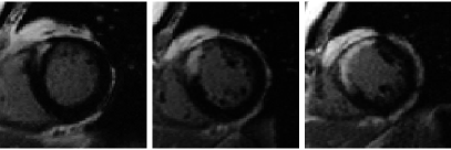
Figure 5 shows three examples of the detected myocardial edge points in SA images. Notably in Fig. 5 (b), where there is a large area of transmural infarcts completely blending in with the BP and surrounding tissues, our method still provides reasonable myocardial edge points because of the smoothness term.

Different from the parameterizing variable used for SA images (i.e., radial angles $\theta$), slice locations $l$ along the normal to the SA image planes are used to parameterize myocardial contours in LA images (Fig. 6 (a)). Hence, myocardial contours are expressed as $\mathcal{C}(l)=(w(l),\,t(l))$. ⁵⁵5Note that in an LA image each $l$ actually defines dual sets of $\mathcal{C}_{\mathrm{endo}}(l)$ and $\mathcal{C}_{\mathrm{epi}}(l)$, as the myocardium is divided into two sides by the central axis of the LV. Since we treat the two sides separately in exactly the same way, we use only one side for the purpose of elaboration. We sample the LA images along rays pointing from the central axis of the LV to beyond the epicardium (Fig. 6 (b)); the samples are denoted as $I_{\mathrm{sample}}(l)$. Again, we devise $I_{\mathrm{templt}}(w,t,s,d)$ with tentative $(w,t,s,d)$ and search for the optimal tetrad which makes $I_{\mathrm{templt}}$ most resemble $I_{\mathrm{sample}}$ for each $l$.

Now two questions are how to estimate: (i) the central axis of the LV, and (ii) reasonable starting points for the search of the optimal $(w,t,s,d)$. To answer both questions, we intersect $\mathcal{C}_{\mathrm{endo,\,rigid}}$ and $\mathcal{C}_{\mathrm{epi,\,rigid}}$ with the LA image planes. The intersection points serve as the initial coarse myocardial edge points in the LA images. Points on the central axis can be easily estimated by averaging the four intersection points on the same SA slices (Fig. 6(c)). The intersections also naturally define the parametrization scheme (i.e., values of $l$) by the relative location of each SA slice with respect to the LA image planes. However, the SA slices are too sparse and thus there are too few $l$’s. On one hand, the SA slices are far away from each other, causing the loss of anatomical continuity of the myocardium; on the other hand, LA images actually contain far more information than what is provided by the intersected locations. In order to retain the natural smoothness of the myocardium and utilize as much information in LA images as possible, we make $l$ denser by linearly interpolating between neighboring SA slices (Fig. 6(d)).

We use the same energy minimization scheme for LA images as for SA images. The energy functional to be minimized still comprises two terms $E_{\mathrm{match}}$ and $E_{\mathrm{smooth}}$ as in (4). $E_{\mathrm{match}}$ stays the same as in (5), except that the parametrization variable is $l$. However, $E_{\mathrm{smooth}}$ in (6) must be slightly adapted to accommodate the shape of the LV in LA images. That is, in LA images $w$ tends to gradually shrink from the base to apex of the LV. Therefore, the first order derivative of $w$ is removed from (6) and $E_{\mathrm{smooth}}$ becomes:

$$E_{\mathrm{smooth}}=\sum_{l}[(w_{ll})^{2}+(t_{l})^{2}+(t_{ll})^{2}].$$

(7)

Several examples of the detected myocardial edge points in LA images are shown in Fig. 7.

Unlike the previous step in which the coarse segmentation is achieved by registration of corresponding cine and LGE images, in this step we directly deform the contours based on local features of the LGE image. We use the simplex mesh (Delingette, 1999) geometry and a Newtonian law of motion to represent and deform the contours. Both endocardial and epicardial surfaces are represented with a simplex mesh respectively, and deformed in an inter-related manner. At each vertex we define three forces, namely, smoothness force $\bm{F}_{\mathrm{smooth}}$, edge attraction force $\bm{F}_{\mathrm{edge}}$ and myocardium thickness force $\bm{F}_{\mathrm{thick}}$. $\bm{F}_{\mathrm{smooth}}$ imposes uniformity of vertex distribution and continuity of simplex angles (Delingette, 1999). $\bm{F}_{\mathrm{edge}}$ draws vertices towards detected myocardial edge points along the normal direction at each vertex. Finally, $\bm{F}_{\mathrm{thick}}$ maintains proper distances between paired endocardial and epicardial vertices. Letting $p^{t}$ denote the position of any vertex at time $t$, the deformation scheme is given by

$$p^{t+1}=p^{t}+(1-\gamma)(p^{t}-p^{t-1})+\alpha\bm{F}_{\mathrm{smooth}}+\beta\bm{F}_{\mathrm{edge}}+\mu\bm{F}_{\mathrm{thick}},$$

(8)

where $\gamma$ is a damping factor, and $\alpha$, $\beta$ and $\mu$ are respective weights.

We initialize the simplex mesh for the epicardium with $\mathcal{C}_{\mathrm{epi,\,rigid}}$ in the steps described below.

Above all, we transform all the involved coordinates to the image coordinate system of the last SA slice. We then re-sample $\mathcal{C}_{\mathrm{epi,\,rigid}}$ with evenly spaced radial angles. The resampling makes the connection relationship among mesh vertices straightforward by aligning all vertices on all slices along the same radial angles, hence simplifying mesh construction. After that we interpolate to obtain several planar contours evenly spaced between the physically existing SA slices. The interpolation is necessary because (i) considering the large distance between neighboring SA slices, properly densified vertices can make $\bm{F}_{\mathrm{smooth}}$ more meaningful; and (ii) some of the interpolated vertices will be attracted by myocardial edge points detected in LA images, which in turn can affect the vertices on the physically existing SA slices through $\bm{F}_{\mathrm{smooth}}$.

Now we specify the connection relationship among vertices. We use the vertices on the two boundary SA slices (the most basal and apical ones) to form two planar 1-simplex meshes (Delingette, 1999), where each vertex is connected to its two immediate neighbors in the image plane. These two 1-simplex meshes act as boundary conditions of the surface mesh. Planar 1-simplex meshes are used to prevent the vertices on the boundaries of the surface mesh from changing their z-values during the deformation; that is, no contraction or elongation of the entire LV in the direction perpendicular to the SA image planes. For interjacent vertices, we follow these rules: (i) vertically, each vertex is connected to its immediate above and below neighbors; (ii) horizontally, each vertex is connected to its immediate left or right neighbor alternatively, i.e., if one vertex is connected to its immediate left neighbor, then the two vertices next to it should be connected to their right neighbors. In simplex-mesh geometry, each vertex can only be connected to three neighbors.

The simplex mesh for the endocardium is initialized in the same way. One exemplary mesh constructed with the above steps is shown in Fig. 8.

As in the original simplex mesh work (Delingette, 1999), we define $\bm{F}_{\mathrm{edge}}$ with the notion of closest points. For each vertex $p_{i}$, we look for the closet pre-detected myocardial edge point $\hat{p}_{i}$ and define the edge attraction force as:

$$\bm{F}_{\mathrm{edge}}=\omega_{i}\ G\left(\frac{(\hat{p}_{i}-p_{i})\cdot\bm{n}_{i}}{D_{\mathrm{cutoff}}}\right)\ \bm{n}_{i},\ \mathrm{where}\ G(x)=\begin{cases}x,&\mathrm{if}\ x\leq 1,\\ 0,&\mathrm{if}\ x>1.\end{cases}$$

(9)

Here, $\omega_{i}$ is a weight between 0 and 1, $\bm{n}_{i}$ the surface normal at vertex $p_{i}$. The gating function $G(x)$ filters out potential outliers specified by the cutoff distance $D_{\mathrm{cutoff}}$ – if the projected distance between $\hat{p}_{i}$ and $p_{i}$ onto $\bm{n}_{i}$ is larger than $D_{\mathrm{cutoff}}$, then $\hat{p}_{i}$ is considered an outlier and has no effect on $p_{i}$. The value of $D_{\mathrm{cutoff}}$ controls the tradeoff between capture range and robustness against outliers during mesh deformation.

$\omega_{i}$ is defined as a normalized sum of first-order and second-order absolute intensity differences at $\hat{p}_{i}$. Recall that $\hat{p}_{i}$ is located on a 1D intensity profile sample $I_{\mathrm{sample}}$. Assuming it is the $j$th pixel on $I_{\mathrm{sample}}$, we calculate the weighted sum $S_{i}=|I_{\mathrm{sample}}(j)-I_{\mathrm{sample}}(j-1)|+|I_{\mathrm{sample}}(j)-I_{\mathrm{sample}}(j+1)|+0.5*|I_{\mathrm{sample}}(j+1)-I_{\mathrm{sample}}(j-1)|$ and define $\omega_{i}$ by:

$$\omega_{i}=\frac{S_{i}-\min(\{S_{k}\})}{\max(\{S_{k}\})-\min(\{S_{k}\})},\ \ k=1,2,\cdots,n,$$

(10)

where $\{S_{k}\}$ is a set of $S_{i}$’s to be normalized together. For SA slices, we process all the detected endocardial edge points of the entire stack as a set, and all the detected epicardial edge points as another set. For LA slices, 4C and 2C images are processed separately. The effects of the weights on the detected myocardial edge points are qualitatively visualized in Fig. 9, where the magnitude of $\omega_{i}$ is coded as brightness of the plot.

In order to define $\bm{F}_{\mathrm{thick}}$, every endocardial vertex is paired with the coplanar epicardial vertex of the same re-sampling angle. Then a vector-based spring force is imposed to maintain the relative position between every pair. Letting $p_{\mathrm{endo}}^{0}$ denote any endocardial vertex before deformation, and $p_{\mathrm{epi}}^{0}$ its paired epicardial vertex, we define $\bm{F}_{\mathrm{thick}}$ as:

$$\begin{split}&\bm{F}_{\mathrm{epi,thick}}=p_{\mathrm{endo}}^{t}+(p_{\mathrm{epi}}^{0}-p_{\mathrm{endo}}^{0})-p_{\mathrm{epi}}^{t},\\ &\bm{F}_{\mathrm{endo,thick}}=p_{\mathrm{epi}}^{t}-(p_{\mathrm{epi}}^{0}-p_{\mathrm{endo}}^{0})-p_{\mathrm{endo}}^{t},\end{split}$$

(11)

where $p_{\mathrm{\ast}}^{t}$ is the vertex after $t$th iteration. $\bm{F}_{\mathrm{thick}}$ is particularly helpful when $\omega_{i}$ is weak at one of the paired vertices but strong at the other. In this case, as a robust supplement to $\bm{F}_{\mathrm{smooth}}$, $\bm{F}_{\mathrm{thick}}$ extrapolates a reasonable position for the vertex of weak $\omega_{i}$ with the original positional relationship between the pair.

With the meshes initialized and the driving forces defined, we can deform the two surface meshes iteratively with (8) ⁶⁶6Because the endocardial and epicardial surfaces are generally smooth with small curvatures everywhere, we do not need the advanced adaptation and refinement algorithms in (Delingette, 1999) and only impose the uniform distribution of vertices via $\bm{F}_{\mathrm{smooth}}$.. In each iteration, we first fix the endocardial mesh and update the epicardial mesh, and then update the endocardial mesh with the epicardial mesh fixed. The deformation is stopped once the movement at any vertex is smaller than 0.1 pixel or the iteration reaches 30 times. A deformed surface mesh is shown in Fig. 8, together with its original shape before deformation. The two meshes obtained after the nonrigid deformation are themselves 3D segmentation of the LV. To obtain the 2D segmentation of each SA image, we simply intersect it with the final meshes.

We have evaluated the proposed 3D segmentation framework with 21 sets of real patient data. The data were acquired with ECG gating by a 1.5T Siemens Symphony MRI scanner from 21 patients (19 males and 2 females, 38-81 years old, mean age $52\pm 10$) three months after their having experienced myocardial infarction, following a bolus injection of gadolinium-based contrast agent. Table 1 shows the sequence parameters used for the data acquisition. Cine and LGE sequences of a same subject comprise the same number of SA slices with the same locations. Depending on the individual heart size, there can be 8-11 SA slices for a patient. In total there were 206 SA slices for all the 21 patients and 158 slices were selected for infarction analysis according to experts’ judgment. While slices (both SA and LA) of the cine sequence comprise 25 frames, slices of the LGE sequence comprise only one frame.

The data were manually analyzed (including segmentation of the myocardium and infarcts) by two experts independently, and the manual contours (denoted by $C_{\mathrm{man}1}$ and $C_{\mathrm{man}2}$) were used as the reference standards in our experiments. The expert who produced $C_{\mathrm{man}1}$ also supervised the production of the a priori segmentation in cine data and had full access to the cine data during his analysis of the LGE data, while the other had no access to the cine data. According to $C_{\mathrm{man}1}$, volumetric percentage of the infarcts with respect to the entire myocardium for the 21 patients ranges from 0 to $35.05\%$ (two cases of non-infarct) with the mean and standard deviation of $18.60\pm 10.43\%$. Five patients had MVO. Using the 16-segments division of the LV recommended by the American Heart Association (AHA; Cerqueira et al., 2002), 160 out of the total $16\times 21=336$ segments (i.e., $47.62\%$) are infarcted, and the locality distribution of the infarctions is charted in Fig. 10.

In the experiments, various parameters introduced in Section 2 are set as follows: (i) For the computation of PI in (1), $r=5$ and $\delta=0.1$. (ii) $w_{\mathrm{d}}$ and $t_{\mathrm{d}}$ in (3) are confined within a narrow band of 7 pixels for SA images and 9 pixels for LA images centered at $w_{\mathrm{0}}$ and $t_{\mathrm{0}}$. (iii) For the energy function in (4), the weight $\lambda$ is set 0.005 for both SA and LA images. (iv) For the 3D deformation scheme in (8), $\gamma=0.7$, $\alpha=0.3$, $\beta=0.3$ and $\mu=0.1$. (v) For the computation of $\bm{F}_{\mathrm{edge}}$ in (9), $D_{\mathrm{cutoff}}=3$. Although the final meshes produced by the 3D deformation scheme are already a 3D segmentation of the LV, we need to intersect them with the SA images to obtain corresponding 2D segmentation contours (denoted by $C_{\mathrm{auto}}$), in order to compare with manual contours drawn by experts in 2D images. Minimum manual adjustments were performed to better evaluate the proposed framework. Of all the 158 SA slices selected for analysis, 3 slices (each from a different volume) were manually reallocated after the automatic misalignment correction, and 8 slices were manually registered due to failure of the automatic translational registration. No manual adjustments were performed on the final $C_{\mathrm{auto}}$.

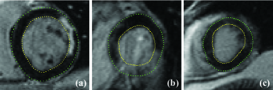
Qualitatively, we observe that segmentation results produced by our framework are consistently accurate for nearly all the LGE images in our database. Figure 11 shows some exemplary results, together with the manual contours delineated by one of the experts. Quantitatively, we have evaluated our framework in terms of both distance- and region-based measures. We have calculated mean distance error and the Dice coefficient (Dice, 1945) between the automatic results and reference standards slice by slice. We have also calculated volumetric Dice coefficients. The results are presented in Table 2. Of the three groups of comparisons, $C_{\mathrm{auto}}$ and $C_{\mathrm{man}1}$ are the most similar with extremely small distances and high slice-wise and volumetric Dice coefficients. Although the difference between $C_{\mathrm{auto}}$ and $C_{\mathrm{man}2}$ is slightly larger, it is very close to the reported inter-observer variations between $C_{\mathrm{man}1}$ and $C_{\mathrm{man}2}$. These results confirm that the myocardial segmentations produced by our framework are close to those obtained by the experts. The general trend that the difference between $C_{\mathrm{auto}}$ and $C_{\mathrm{man}1}$ is smaller than between $C_{\mathrm{auto}}$ and $C_{\mathrm{man}2}$ is not surprising, because the expert who produced $C_{\mathrm{man}1}$ also supervised the a priori segmentation of the cine data. On the contrary, the other expert had no such a priori knowledge and had to guess based on her experience when the contrast is poor.

It is difficult to quantitatively compare the accuracy of our 3D segmentation framework with those of the existing methods (Ciofolo et al., 2008; Dikici et al., 2004). Given that different data sets were used, it is inappropriate to directly compare accuracies or errors reported in the papers. However, qualitatively we have identified the following advantages of our 3D segmentation method over others.

First, compared to pure 2D segmentation methods (Dikici et al., 2004; Wei et al., 2011) which merely produce discrete cylinders in 3D space (Fig. 12(a)), our 3D segmentation framework produces more accurate 3D reconstruction of the LV geometry (Fig. 12(b)). Moreover, the 3D smoothness force $\bm{F}_{\mathrm{smooth}}$ helps extrapolate reasonable myocardial boundaries with information from the LA and neighboring SA slices, when the current slice lacks contrast.

Second, though the work by Ciofolo et al. (2008) also involved deforming 3D meshes for segmentation, the meshes were attracted only to features detected in SA LGE images. Due to the large anisotropy of the stacks of SA images, a respectable portion of the vertices was moved by only regulating forces because there were no feature points lying between the SA slices (Fig. 13 (a)). In contrast, since we incorporate the two standard LA views (4C and 2C) into our 3D segmentation framework, a considerable amount of feature points detected in the LA images fill the gaps (Fig. 13 (b)). These extra feature points can make the final meshes represent the physical shape of the scanned LV with higher fidelity. The 2D segmentation contours in SA images obtained by intersection with the meshes can also be more accurate, because the extra information contained between the SA images is propagated over the meshes by $\bm{F}_{\mathrm{smooth}}$ (Delingette, 1999).

Third, the work by Ciofolo et al. (2008) did not mention any correction of the misalignment artifacts for stacks of LGE images. This exposes the reconstructed 3D representation of the LV to potential distortion (McLeish et al., 2002). In contrast, we realign all the SA and LA slices in the original patient coordinate system prior to the construction and deformation of the meshes, thus endowing the 3D segmentation with higher fidelity.

We also evaluated our framework on simulated data generated from the 4D XCAT male phantom (Segars et al., 2010). The LGE data are simulated as follows. First a voxelized torso phantom with an isotropic voxel size of 1.34 mm is generated from the XCAT. Nine tissues are included: the myocardium, infarct, blood, pericardium, lung, spleen, liver, stomach and the rest of the body. An expert manually delineated regions for each tissue in a set of real patient data. Then every voxel in the torso phantom is randomly assigned a value according to its tissue type. The assigned value is uniformly sampled from the regions of the specified tissue. Two exceptions are the infarct and body: voxels of these two tissues are assigned mean values of the respective regions. After that, simulated images of standard CMR orientations (SA, 4C and 2C) with the same slice dimensions as our real data (pixel spacing = 1.34 mm, slice thickness and spacing = 7 and 3 mm, resulting in 8 SA slices) are reconstructed from the torso volume. Each simulated image is an average of the intensities within its slice thickness to increase the signal to noise ratio. The cine data are simulated in the same way, except that no infarct is included. Figure 14 shows several examples of the simulated cine and LGE data.

To create enough difference in myocardium shape between the LGE and cine SA images, the LGE and cine data were simulated at different cardiac and respiratory phases. The infarcts were set at mid-ventricle, spanning 50 mm along the LA of the LV. Four LV volumes with infarcts located at anterior, lateral, inferior and septal walls respectively were simulated. The infarcts span 100 degrees on the myocardial circumference and are 100% transmural. Myocardial contours of the simulated data were derived from the original voxelized phantom. The cine contours are used as the a priori segmentation to our segmentation framework, while the LGE contours are used as the ground truth ($C_{\mathrm{grnd}}$) for evaluation.

The various parameters are set to the same as presented in Section 3.1.2. No manual adjustment was performed to the simulated data.

The segmentation results obtained by an expert and our framework on the simulated LGE data are shown in Table 3. Both manual and automatic segmentations are very close to the ground truth, and the difference between the two segmentations is also small. What is noteworthy is the standard deviation of the slice-wise Dice coefficients for the BP between $C_{\mathrm{auto}}$ and $C_{\mathrm{grnd}}$, which is significantly higher than the others. This is caused by the most apical slice in each volume and can be explained by three facts regarding very apical slices: (i) the myocardium is usually much blurred; (ii) the apex’s motion is large and causes a big change between the myocardium shape in cine and LGE images; (iii) areas of the myocardium are small and the Dice coefficient is known to be sensitive to small areas. In fact segmentation of the myocardium in very apical slices is always so difficult that no method can consistently produce reliable results. In practice, we provide a simple user correction scheme to effectively handle such cases. The mean Dice coefficient for the BP between $C_{\mathrm{auto}}$ and $C_{\mathrm{grnd}}$ becomes $96.97\pm 1.50\%$ if the most apical slice in each volume is excluded.

In this experiment, one observer manually drew the myocardial contours for the selected SA cine images that correspond to the target LGE images, serving as the manual a priori segmentation (denoted by $A_{\mathrm{manu}}$). Meanwhile, the automatically generated cine contours used in Section 3.1 (denoted by $A_{\textrm{auto}}$) serve as the control group. Segmentation accuracies with $A_{\mathrm{manu}}$ and $A_{\mathrm{auto}}$ as a priori are compared to test whether the segmentation framework can produce consistently good results with both manually drawn and automatically generated a priori segmentations. The results are presented in Table 4. As we can see, the segmentation results with both kinds of inputs are similarly good, though the results produced with $A_{\mathrm{manu}}$ are slightly better. This indicates that our framework can consistently produce high quality segmentation for LGE images despite that in practice the potential a priori segmentation in the corresponding cine images can be either manually drawn or (semi-) automatically generated.

In this experiment, $A_{\mathrm{manu}}$ is purposely enlarged and shrunk by 1 mm to generate two sets of artificially simulated a priori segmentations – $A_{\mathrm{enlg}}$ and $A_{\mathrm{shrk}}$. Differences between segmentation results with $A_{\mathrm{enlg}}$ and $A_{\mathrm{shrk}}$ as a priori segmentations are examined to test the consistency of our segmentation framework given the a priori segmentations 2 mm apart from each other. The comparison is presented in Table 5. Mean distances between the segmentation results are greatly decreased from the mean distances between the two a priori themselves. Area similarity is also improved, which is revealed by the fact that Dice coefficients evaluated at all three levels are significantly increased. The comparison results further validate the consistency of our segmentation framework – it can produce consistent segmentations even with varied a priori in the range of 2 mm.

The experimental results have shown that our framework can produce highly consistent segmentations despite that the given a priori segmentation in cine images can vary. The consistency and robustness are important and desirable because both inter-observer variability and automatic segmentation accuracies for cine images are in the range of 1-2 mm (Petitjean and Dacher, 2011). Although starting with propagating the a priori segmentation contours from cine images, the consistency of our segmentation framework makes it possible to obtain highly reproducible segmentation of LGE images given different a priori segmentations (either manual or automatic) in cine images.

References

- Abdel-Aty and Tillmanns (2010) Abdel-Aty, H., Tillmanns, C., 2010. The use of cardiovascular magnetic resonance in acute myocardial infarction. Curr Cardiol Rep 12, 76–81.
- Barajas et al. (2006) Barajas, J., Caballero, K., Barnés, J., Carreras, F., Pujadas, S., Radeva, P., 2006. Correction of misalignment artifacts among 2-D cardiac MR images in 3-D space, in: First International Workshop on Computer Vision for Intravascular and Intracardiac Imaging, MICCAI 2006, pp. 114–121.
- Cerqueira et al. (2002) Cerqueira, M.D., Weissman, N.J., Dilsizian, V., Jacobs, A.K., Kaul, S., Laskey, W.K., Pennell, D.J., Rumberger, J.A., Ryan, T., Verani, M.S., 2002. Standardized Myocardial Segmentation and Nomenclature for Tomographic Imaging of the Heart. Circulation 105, 539–542.
- Chen et al. (2008) Chen, T., Babb, J., Kellman, P., Axel, L., Kim, D., 2008. Semiautomated Segmentation of Myocardial Contours for Fast Strain Analysis in Cine Displacement-Encoded MRI. IEEE Trans Med Imaging 27, 1084 –1094.
- Ciofolo et al. (2008) Ciofolo, C., Fradkin, M., Mory, B., Hautvast, G., Breeuwer, M., 2008. Automatic myocardium segmentation in late-enhancement MRI, in: IEEE ISBI ’08, pp. 225–228.
- Delingette (1999) Delingette, H., 1999. General object reconstruction based on simplex meshes. Int J Comput Vis 32, 111–146.
- Dice (1945) Dice, L., 1945. Measures of the amount of ecologic association between species. Ecology 26, 297–302.
- Dikici et al. (2004) Dikici, E., O’Donnell, T., Setser, R., White, R.D., 2004. Quantification of Delayed Enhancement MR Images, in: Barillot, C., Haynor, D.R., Hellier, P. (Eds.), MICCAI 2004. Springer Berlin / Heidelberg. volume 3216 of LNCS, pp. 250–257.
- Elagouni et al. (2010) Elagouni, K., Ciofolo-Veit, C., Mory, B., 2010. Automatic segmentation of pathological tissues in cardiac MRI, in: IEEE ISBI ’10: From Nano to Macro, pp. 472–475.
- Hautvast et al. (2006) Hautvast, G., Lobregt, S., Breeuwer, M., Gerritsen, F., 2006. Automatic contour propagation in cine cardiac magnetic resonance images. IEEE Trans Med Imaging 25, 1472–1482.
- Hennemuth et al. (2008) Hennemuth, A., Seeger, A., Friman, O., Miller, S., Klumpp, B., Oeltze, S., Peitgen, H.O., 2008. A Comprehensive Approach to the Analysis of Contrast Enhanced Cardiac MR Images. IEEE Trans Med Imaging 27, 1592 –1610.
- Hsu et al. (2006) Hsu, L.Y., Natanzon, A., Kellman, P., Hirsch, G.A., Aletras, A.H., Arai, A.E., 2006. Quantitative myocardial infarction on delayed enhancement MRI. Part I: Animal validation of an automated feature analysis and combined thresholding infarct sizing algorithm. J Magn Reson Imaging 23, 298–308.
- Hunold et al. (2005) Hunold, P., Schlosser, T., Vogt, F., Eggebrecht, H., Schmermund, A., Bruder, O., Schuler, W., Barkhausen, J., 2005. Myocardial late enhancement in contrast-enhanced cardiac MRI: distinction between infarction scar and non-infarction-related disease. AJR Am J Roentgenol 184, 1420.
- Kaftan et al. (2009) Kaftan, J.N., Tek, H., Aach, T., 2009. A two-stage approach for fully automatic segmentation of venous vascular structures in liver CT images, in: Pluim, J.P.W., Dawant, B.M. (Eds.), Medical Imaging 2009: Image Processing, SPIE, Orlando, USA. pp. 725911–1–12.
- Kolipaka et al. (2005) Kolipaka, A., Chatzimavroudis, G.P., White, R.D., O’Donnell, T.P., Setser, R.M., 2005. Segmentation of non-viable myocardium in delayed enhancement magnetic resonance images. Int J Cardiovasc Imaging 21, 303–311. 10.1007/s10554-004-5806-z.
- Li et al. (2009) Li, C., Jia, X., Sun, Y., 2009. Improved semi-automated segmentation of cardiac CT and MR images, in: ISBI ’09: From Nano to Macro, pp. 25–28.
- Lötjönen et al. (2004) Lötjönen, J., Pollari, M., Kivistö, S., Lauerma, K., 2004. Correction of Movement Artifacts from 4-D Cardiac Short- and Long-Axis MR Data, in: Barillot, C., Haynor, D., Hellier, P. (Eds.), MICCAI 2004. Springer Berlin / Heidelberg. volume 3217 of Lecture Notes in Computer Science, pp. 405–412.
- McLeish et al. (2002) McLeish, K., Hill, D., Atkinson, D., Blackall, J., Razavi, R., 2002. A study of the motion and deformation of the heart due to respiration. IEEE Trans Med Imaging 21, 1142 –1150.
- Moore et al. (2003) Moore, J., Drangova, M., Wierzbicki, M., Barron, J., Peters, T., 2003. A High Resolution Dynamic Heart Model Based on Averaged MRI Data, in: Ellis, R., Peters, T. (Eds.), MICCAI 2003. Springer Berlin / Heidelberg. volume 2878 of Lecture Notes in Computer Science, pp. 549–555.
- Otsu (1979) Otsu, N., 1979. A threshold selection method from gray-level histograms. IEEE Trans Syst, Man Cybern 9, 62–66.
- Petitjean and Dacher (2011) Petitjean, C., Dacher, J.N., 2011. A review of segmentation methods in short axis cardiac mr images. Medical Image Analysis 15, 169 – 184.
- Reimer et al. (1979) Reimer, K., Jennings, R., et al., 1979. The “wavefront phenomenon” of myocardial ischemic cell death. II. Transmural progression of necrosis within the framework of ischemic bed size (myocardium at risk) and collateral flow. Lab Invest 40, 633–644.
- Segars et al. (2010) Segars, W.P., Sturgeon, G., Mendonca, S., Grimes, J., Tsui, B.M., 2010. 4D XCAT phantom for multimodality imaging research. Med Phys 37, 4902–4915.
- Studholme et al. (1999) Studholme, C., Hill, D.L.G., Hawkes, D.J., 1999. An overlap invariant entropy measure of 3d medical image alignment. Pattern Recognition 32, 71 – 86.
- Tao et al. (2010) Tao, Q., Milles, J., Zeppenfeld, K., Lamb, H., Bax, J., Reiber, J., van der Geest, R., 2010. Automated segmentation of myocardial scar in late enhancement MRI using combined intensity and spatial information. Magn. Reson. Med. 64, 586–594.
- Valindria et al. (2011) Valindria, V.V., Angue, M., Vignon, N., Walker, P.M., Cochet, A., Lalande, A., 2011. Automatic Quantification of Myocardial Infarction from Delayed Enhancement MRI, in: Signal-Image Technology and Internet-Based Systems (SITIS), 2011 Seventh International Conference on, pp. 277 –283.
- Vu et al. (2007) Vu, N., Ghosh, P., Manjunath, B., 2007. Retina layer segmentation and spatial alignment of antibody expression levels, in: IEEE ICIP 2007, pp. II –421 –II –424.
- Weese et al. (1997) Weese, J., Buzug, T., Lorenz, C., Fassnacht, C., 1997. An approach to 2D/3D registration of a vertebra in 2D x-ray fluoroscopies with 3D CT images, in: Troccaz, J., Grimson, E., Mösges, R. (Eds.), CVRMed-MRCAS’97. Springer Berlin / Heidelberg. volume 1205 of LNCS, pp. 119–128.
- Wei et al. (2011) Wei, D., Sun, Y., Chai, P., Low, A., Ong, S., 2011. Myocardial Segmentation of Late Gadolinium Enhanced MR Images by Propagation of Contours from Cine MR Images, in: Fichtinger, G., Martel, A., Peters, T. (Eds.), MICCAI 2011. Springer Berlin / Heidelberg. volume 6893 of Lecture Notes in Computer Science, pp. 428–435.
- Zadicario et al. (2008) Zadicario, E., Avidan, S., Shmueli, A., Cohen-Or, D., 2008. Boundary snapping for robust image cutouts, in: IEEE CVPR 2008, pp. 1 –8.