Three dimensional magnetorotational core-collapse supernova explosions of a 39 solar mass progenitor star
Abstract
We perform three-dimensional simulations of magnetorotational supernovae using a progenitor star with two different initial magnetic field strengths of G and G in the core. Both models rapidly undergo shock revival and their explosion energies asymptote within a few hundred milliseconds to values of erg after conservatively correcting for the binding energy of the envelope. Magnetically collimated, non-relativistic jets form in both models, though the jets are subject to non-axisymmetric instabilities. The jets do not appear crucial for driving the explosion, as they only emerge once the shock has already expanded considerably. Our simulations predict moderate neutron star kicks of about , no spin-kick alignment, and rapid early spin-down that would result in birth periods of about , too slow to power an energetic gamma-ray burst jet. More than of iron-group material are ejected, but we estimate that the mass of ejected will be considerably smaller as the bulk of this material is neutron-rich. Explosive burning does not contribute appreciable amounts of because the burned material originates from the slightly neutron-rich silicon shell. The iron-group ejecta also show no pronounced bipolar geometry by the end of the simulations. The models thus do not immediately fit the characteristics of observed hypernovae, but may be representative of other transients with moderately high explosion energies. The gravitational-wave emission reaches high frequencies of up to 2000 Hz and amplitudes of over 100 cm. The gravitational-wave emission is detectable out to distances of Mpc in the planned Cosmic Explorer detector.
keywords:
transients: supernovae – gravitational waves1 Introduction
Core-collapse supernovae (CCSNe), the explosions of stars massive enough to develop an iron core, are some of the most violent events in the Universe. They result in a brilliant optical outburst that can reach the brightness of an entire galaxy for weeks, and they emit an enormous amount of energy, several erg, in the form of neutrinos as well as erg in the form of gravitational waves (GWs), making them a perfect target for multi-messenger astronomy.
In regular CCSNe, shock revival is likely achieved by neutrino heating. In recent years, significant progress has been made in 3D modelling of non-rotating neutrino-driven CCSNe, which has considerably enhanced our understanding of CCSN explosion properties, multi-messenger observables, and neutron star and black hole birth masses, spins and kicks (see recent reviews Kalogera et al. 2019; Abdikamalov et al. 2020; Müller 2020; Burrows & Vartanyan 2021). However, even though the neutrino-driven mechanism can explain explosions with ejecta kinetic energies up to erg, there is a class of considerably more energetic “hypernovae” with energies of about erg; observationally these are classified as broad-lined Ic supernovae (Type Ic-BL; Woosley & Bloom, 2006; Gal-Yam, 2017). These explosions, which sometimes are accompanied by long gamma-ray bursts (GRB), are likely explained by some form of magnetohydrodynamic (MHD) mechanism that taps the energy of a rapidly spinning millisecond magnetar (Bisnovatyi-Kogan et al., 1976; Duncan & Thompson, 1992; Usov, 1992; Akiyama et al., 2003) or a black hole accretion disk in the collapsar scenario (MacFadyen & Woosley, 1999).
Hypernovae are of interest beyond supernova theory. Since the hypernova rate is significantly higher at low metallacity, the explosions may have played a key role for the enrichment of the Milky Way with heavy elements in its early history as major production sites for elements like zinc (Nomoto et al., 2006; Kobayashi et al., 2006) and possible rapid-neutron capture process elements (Winteler et al., 2012; Mösta et al., 2018; Grimmett et al., 2021a; Reichert et al., 2022).
MHD explosions with detailed neutrino transport have been investigated in a large number of 2D simulations (Burrows et al., 2007; Obergaulinger & Aloy, 2017; Reichert et al., 2021; Grimmett et al., 2021b; Jardine et al., 2022). However, the assumption of 2D axisymmetry is a significant concern for accurate explosion dynamics and nucleosynthesis predictions, as it it prohibits the development of any kink instability of MHD jets (Mösta et al., 2014) and also inhibits Kelvin-Helmholtz instability between outflows and downflows at high Mach number.
In recent years, 3D MHD simulations of magnetorotational explosions have become available (Winteler et al., 2012; Mösta et al., 2014; Mösta et al., 2018; Kuroda et al., 2020; Obergaulinger & Aloy, 2020; Kuroda et al., 2020; Bugli et al., 2021). However, few of the existing 3D MHD models (some with relatively coarse spatial resolution) include detailed multi-group neutrino transport as yet (Kuroda et al., 2020; Obergaulinger & Aloy, 2020; Bugli et al., 2021), which is critical for correctly predicting the composition of the magnetically-driven outflows. Although a first nucleosynthesis study based on 3D hypernova models with detailed neutrino transport is now available (Reichert et al., 2022), further simulations are desirable. A better understanding of seed fields in the progenitor is also needed to fully understand magnetorotational explosions. Currently, 3D progenitor models with magnetic fields are only available for non-rotating progenitors (Varma & Müller, 2021). A few studies of the impact of different magnetic field configurations have also been carried out by Bugli et al. (2020); Aloy & Obergaulinger (2020).
From the perspective of gravitational-wave (GW) astronomy, it is noteworthy that the majority of the recent long-duration 2D and 3D CCSN MHD simulations have not discussed predictions of the GW emission during the post-bounce phase with the exception of the 2D study of Jardine et al. (2022). In recent years, the Advanced LIGO (LIGO Scientific Collaboration et al., 2015) and Virgo (Acernese et al., 2015) GW detectors have detected GWs from compact binary sources in increasing numbers (Abbott et al., 2019, 2021a; The LIGO Scientific Collaboration et al., 2021). As the detectors sensitivity increases over the coming years, the chance of detecting GWs from another source, like a CCSN, significantly increases.
Different from ordinary CCSNe, the GW signals from MHD explosions may be loud enough to be detected outside the Milky Way by current generation detectors (Gossan et al., 2016; Abbott et al., 2020; Szczepańczyk et al., 2021). However, those detection studies only include the core-bounce part of MHD signals, as longer duration GW signals from MHD simulations were not available at the time, resulting in their detection distances being only a lower limit. The GW core-bounce signal has been extensively studied and may inform us of the progenitor rotation rate and nuclear equation of state properties (Obergaulinger et al., 2006; Dimmelmeier et al., 2008; Scheidegger et al., 2008; Takiwaki & Kotake, 2011; Abdikamalov et al., 2014; Fuller et al., 2015; Richers et al., 2017; Edwards, 2021). However, the full GW signal in the MHD case must be predicted in order for us to perform more accurate detection studies and understand the relationship between the GW signal morphology and the astrophysics of the source. 2D simulations (Jardine et al., 2022) have provided a first glimpse at the GW signal from the post-bounce phase over several hundreds of milliseconds, but suffer from the inherent limitations as discused before. On even longer time scales, anelastic 3D simulations have addressed GW emission due to PNS convection and revealed interesting signal features (Raynaud et al., 2022). The GW emission from the very dynamical early explosion phase of magnetorotational CCSNe also needs to be studied based on 3D MHD simulations of the first few hundred milliseconds after shock revival.
There are already cogent reasons to anticipate that the GW emission from the post-bounce phase of magnetorotational explosions is quantitatively important and may differ in important respects from the post-bounce GW emission in neutrino-driven CCSNe. In the GW signatures of 3D neutrino-driven explosion models, common features have been identified and linked to the explosion and PNS properties through quantitative relations for their characteristics frequencies. The GW f/g-mode frequency (Müller et al., 2013; Morozova et al., 2018; Torres-Forné et al., 2018; Sotani & Takiwaki, 2016), which produces a conspicuous emission band at a few to about , can be described by universal relations that depend on the mass and frequency of the PNS (Torres-Forné et al., 2019). Similarly, low-frequency emission in models with strong activity of the standing accretion shock instability (SASI: Blondin et al., 2003; Blondin & Mezzacappa, 2006; Foglizzo et al., 2007) will reflect the SASI frequency, which is determined by the shock radius and the radius of the PNS (Müller & Janka, 2014). 3D simulations have already demonstrated that rotation alone already quantitatively affects the post-bounce GW emission (Andresen et al., 2019; Pajkos et al., 2019; Kuroda et al., 2014; Shibagaki et al., 2020; Powell & Müller, 2020) and can break the familiar relation between neutron star parameters and the f/g-mode frequency (Powell & Müller, 2020). For rapid rotation, qualitatively new emission features from non-axisymmetric instabilities can arise (Kuroda et al., 2014; Shibagaki et al., 2020). When both rotation and magnetic fields are taken into account, Jardine et al. (2022) found a significant impact on the time-frequency structure of the GW signal both for models with rapid rotation or strong initial field strengths in a small 2D parameter study. As the next step, 3D simulations are needed to thoroughly understand the effect of rotation and magnetic fields on the post-bounce GW emission and to potentially identify new signal features.
In this paper, we perform two 3D simulations using the MHD version of the CoCoNuT-FMT code with a pseudo-relativistic potential to mimic the effects of relativistic gravity. We simulate magnetorotational explosions of a rapidly rotating progenitor star (Aguilera-Dena et al., 2018) with two different magnetic field strengths ( G and G at the centre of the star). We compare the results of our models to the previous 3D hydrodynamic simulation of the progenitor star without magnetic fields in Powell & Müller (2020), and the 2D simulations of the same progenitor model in Jardine et al. (2022).
In Section 2, we give a brief description of the progenitor model and the MHD code used in our simulations. In Section 3, we describe the impact of the rotation and magnetic fields on the explosion dynamics and jets. The remnant properties are discussed in Section 4 with a particular view to the millisecond-magnetar scenario for long gamma-ray bursts. We study the ejecta composition and geometry of our models in Section 5. In Section 6, we discuss the GW emission and the prospects for detection. A summary and conclusions are given in Section 7.
2 Progenitor model and simulation methodology
We perform two 3D simulations of the B-series model with an initial mass of from Aguilera-Dena et al. (2018) evolved using the stellar evolution code MESA (Paxton et al., 2011; Paxton et al., 2013, 2015, 2018). Similar models are also presented in (Aguilera-Dena et al., 2020). Due to rapid rotation, this model evolved quasi-chemically homogeneously and developed a large CO core of . Mass loss reduces the pre-collapse mass of the progenitor star to . It is rapidly rotating with an initial surface rotational velocity of , a pre-collapse core rotation rate (angular velocity) of , and a low metallicity of . Despite its large CO core mass, the progenitor only has a moderately high pre-collapse compactness parameter (O’Connor & Ott, 2011) of .
The progenitor model was previously simulated in 3D by Powell & Müller (2020) with the same rotation profile, but neglecting magnetic fields. Their simulation was performed with the general relativistic version of the neutrino hydrodynamics code CoCoNuT-FMT (Müller et al., 2010; Müller & Janka, 2015). The model developed a strong neutrino-driven explosion without the aid of magnetic fields. Where relevant, we include some of the results from this non-magnetic model in our paper for a comparison to our new models. We label this reference model m39_B0.
In our two new 3D simulations, we add initial magnetic fields to the model. We impose a dipolar field with two different field strengths, peaking at G and G for both the poloidal and toroidal component at the centre of the star. Following Suwa et al. (2007); Varma et al. (2021), the field is derived from the vector potential
| (1) |
where is the maximum poloidal and toroidal field strength, and the radius parameter is set to . We refer to the models with and as m39_B12 and m39_B10, respectively. The dynamo model used for the progenitor evolution predicts toroidal field strengths of up to and poloidal field strengths of up at mass coordinates of . Throughout most of the core, however, the field strengths are significantly lower with typical values of for the toroidal field and as low as for the poloidal field. The choice of relatively large fields with a higher poloidal-to-toroidal field ratio in the simulations is motivated by several considerations. The high numerical resolution required to self-consistently follow the emergence of the requisite strong poloidal field from realistic, toroidally-dominated progenitor fields for jet-driven explosions by post-collapse amplification processes (Mösta et al., 2015) is not currently affordable in global long-time simulations with neutrino transport. It is therefore common practice to mimic the assumed strong-field conditions resulting from dynamo processes by imposing strong seed fields as initial conditions. Second, the simple dynamo models in spherically symmetric stellar evolution codes only provide effective mean-field values for the poloidal and toroidal field, but not the detailed field geometry needed for 3D simulations (although more sophisticated models of magnetorotational stellar evolution may provide more information, see Takahashi & Langer, 2021). Finally, 3D simulations of magnetoconvection in CCSN progenitors suggest that current stellar evolution models may underestimate magnetic field strengths (Varma & Müller, 2021). Given the uncertainties about the magnetic fields in the progenitor stars and post-collapse field amplification processes, the current models remain scenarios for the case of rapid explosions due to fast field amplification or strong progenitor fields, rather than genuine predictions based on first principles.
The m39_B12 model was simulated up to 0.68 s after core bounce, and the m39_B10 model was simulated up to 0.33 s after core bounce due to less available computater time. The collapse was followed in axisymmetry, and the models were mapped to 3D shortly after bounce.
We perform our simulations using the MHD version of CoCoNuT-FMT as described in Müller & Varma (2020). The code solves the Newtonian MHD equations using the HLLC solver (Gurski, 2004; Miyoshi & Kusano, 2005) and hyperbolic divergence cleaning (Dedner et al., 2002). The MHD equations for the density , magnetic field , total energy density , velocity and Lagrangian multiplier are expressed in Equations (2)–(6) in Gaussian units including divergence cleaning terms as
| (2) | ||||
| (3) | ||||
| (4) | ||||
| (5) | ||||
| (6) |
Here denotes the hyperbolic cleaning speed, the gas pressure, the damping time for the Lagrangian multiplier, and and are the neutrino energy and momentum source terms. The cleaning speed is identified with the fast magnetosonic velocity, and the damping time is set to eight times the magnetosonic crossing time of a cell. The effective potential of Müller et al. (2008) is used to approximate the effects of relativistic gravity. In comparing to the reference model m39_B0, the use of a pseudo-Newtonian treatment as opposed to the general relativistic reference simulation of model m39_B0 can lead to small systematic differences, e.g., in proto-neutron star structure and hence in global proto-neutron star parameters like its total mass.
Neutrinos are treated using the FMT (Fast Multi-group Transport) method of Müller & Janka (2015). The effects of relativistic gravity are approximately taken into account by means of a modified gravitational potential (Müller et al., 2008), and are also included as gravitational redshift in the neutrino transport. The GW emission is extracted by the time-integrated quadrupole formula (Finn, 1989; Finn & Evans, 1990; Blanchet et al., 1990).
The models have a grid resolution of zones in radius, latitude and longitude. The grid reaches out to km, and 21 energy zones are used in the transport solver. To save computer time, we follow the collapse phase in axisymmetry (2D) and map to 3D shortly after bounce, imposing small random seed perturbation to trigger the growth of non-axisymmetric modes.
We use the Lattimer & Swesty (1991) equation of state, with a bulk incompressibility parameter of K=220 MeV. At low densities, we use an equation of state accounting for photons, electrons, positrons and an ideal gas of nuclei together with a flashing treatment for nuclear reactions (Rampp & Janka, 2002). The flashing scheme burns to above temperatures of ; , and to above and nuclei below the iron group to above . Above (i.e., ), the code uses a nuclear statistical equilibrium (NSE) table comprising neutron, protons, , , , , , , , , , , , , , , , and (as representative “dummy” nuclei for very neutron-rich conditions) and (Buras et al., 2006a). The inclusion of several iron-group nuclei with a different neutron-to-proton-ration allows us to roughly estimate whether ejeected iron-group elements are likely in the form of (for electron fraction , Hartmann et al., 1985; Wanajo et al., 2018) or in the form of more neutron-rich nuclei.
3 Explosion dynamics and morphology


The minimum and maximum shock radius of the two magnetised models and their non-magnetised counterpart are shown in Figure 1. The shock is revived at a similar early time for both magnetised models, and about 100 ms earlier than the m39_B0 model from Powell & Müller (2020). Earlier explosion times for models with stronger magnetic fields are consistent with the findings of previous work (Obergaulinger et al., 2014; Obergaulinger & Aloy, 2022a). Early shock revival in model m39_B10 is noteworthy, because the behaviour for moderately high initial fields is markedly different from 2D models of the same progenitor (Jardine et al., 2022). In the 2D models of Jardine et al. (2022), the m39_B12 model undergoes shock revival at a similarly early time, but their 2D version of m39_B10 undergoes shock revival much later at ms after bounce, i.e., later than in 3D and later than the corresponding non-magnetised model.
We compute the diagnostic explosion energy following Buras et al. (2006b); Varma et al. (2022) by integrating the total thermal, kinetic, magnetic, and potential energy over the region that is nominally unbound,
| (7) |
The explosion energies are shown in Figure 1. The magnetic models m39_B12 and m39_B10 reach a significantly higher explosion energy than the neutrino-driven model m39_B0. The m39_B12 model reaches energies of erg by the end of the simulation, and model m39_B10 reaches erg. Moreover, whereas gradually increases in model m39_B0 over the duration of the entire simulation and clearly has not saturated yet, the explosion energy increases rapidly in models m39_B10 and m39_B12 around ms after bounce and then starts to plateau at ms (although m39_B12 has just about reached this point). Our results put models m39_B12 and m39_B10 in the realm of hypernovae, albeit still quite far from the most energetic ones with energies of erg. However, the final explosion energy is still uncertain because the material ahead of the shock still has a binding energy (“overburden”) of . There is no straightforward means of estimating the final explosion energy, although subtracting the overburden from the diagnostic explosion energy has worked well for long-time models of fallback explosions (Chan et al., 2020).
Although the inclusion of magnetic fields clearly has a significant impact on shock revival, models m39_B12 and m39_B10 do not conform to the classical picture of magnetorotational explosions driven by bipolar jets initially. Instead, the shock already expands significantly in both models before jets truly start to emerge, at which point shock expansion accelerates. The development of the explosion morphology is illustrated by Figures 2 and 3, which show 2D slices of the specific entropy for model m39_B12 and model m39_B10, respectively.
In model m39_B12, the shock expands to about before jets develop along both directions of the rotation axis around , i.e., at the time corresponding to the visible break in the shock trajectory. The jets remain rather unstable and show intermittent activity. By 200 ms after bounce, the jet in the North direction disappears and a strong jet is only visible in the South direction. The jet direction vacillates visibly, indicating kink instability (Eichler, 1993; Begelman, 1998) as in previous 3D simulations of magnetorotational CCSNe (Mösta et al., 2014; Kuroda et al., 2020; Obergaulinger & Aloy, 2020, 2021a; Bugli et al., 2021; Bugli et al., 2022), which will be analysed further below. The intermittency of the jet and the instability of the jet direction may be unrelated phenomena, however (see below).
In model m39_B10, jet formation is delayed considerably longer; no jet is visible yet at 150 ms. At 200 ms after core bounce, the model develops a strong jet in both directions. Although the jets are very narrow at their base, and somewhat close to being constricted by surrounding material at radii of several hundred km, they remain more stable than in m39_B12 and grow continuously until the end of the simulation. The variations in jet strength are most reminiscent of sausage instability than of kink instability in this model, but the extreme narrowness of the jets (with a width of only a few grid cells) calls for caution in interpreting the jet morphology.
Following previous studies (Mösta et al., 2014; Kuroda et al., 2020; Obergaulinger & Aloy, 2020, 2021a; Bugli et al., 2021), we further quantify the development of jet instabilities by determining the displacement of the barycentre of the magnetic energy from the z-axis,
| (8) |
where the integration is restricted to a region around the axis and outside the neutron star (such as to cover only one lobe of the jet). Following closely the method of Kuroda et al. (2020), we integrate over a region within 50 km of the axis and , i.e., slices at at constant radial coordinate through the jet rather than an extended volume containing the entire jet. To interpret the nature of the instability, we also examine the toroidal-to-poloidal field ratio , which determines the growth rate and critical wavelength of the kink mode under for idealised setups (Kruskal & Tuck, 1958; Begelman, 1998; Mösta et al., 2014),
| (9) |
where is the width of the jet (pinch). We quantify this by integrating and over the same area,
| (10) |
The results for the jet displacement and the ratio are shown in Figure 4 and quantitatively confirm the presence of jet instability. For both models, the position of the barycentre rapidly varies on short time scales with frequent excursions to until , corresponding to a deviation of the jet direction from the axis by . Larger displacements are seen in model m39_B12 (which has been run longer) at later times. In model m39_B12, the trajectories of the barycentre circle the axis, consistent with the helical deformation expected from the kink instability. The numerical values of are well above unity at early times and then decrease to by in m39_B10 and by in m39_B12, which indicates that the kink instability can indeed develop on short wavelengths. It is puzzling, however, that the jet instability becomes more pronounced in model m39_B12 at late times when than at earlier when is larger. This behaviour may be related to changes in other jet parameters and the environment of the jet. It is suggestive that the phase of more vigorous jet instability coincides with the onset of the plateau in the explosion energy, but this may be a coincidence. Based on the critical wavelength for instability predicted by the Kruskal-Shafranov criterion, we also raise resolution effects as a potential caveat. With peak values of , we expect unstable modes with a wavelength of the order of the width of the jet, which amounts to just a few zones; hence the growth of the kink instability is likely somewhat affected by numerical dissipation. Moreover, the behaviour of the kink instability may be affected by the spherical polar grid geometry. While our models confirm that spherical polar grids can qualitatively capture the kink instability at the current resolution, and are better resolved than some other models using a spherical grid geometry (Obergaulinger & Aloy, 2022a; Bugli et al., 2022), future code comparisons and resolution studies should assess the requirements for capturing the kink instability at the level required for predictive hypernova models.
Even though it may be tempting to also associate the intermittency of the jet (which is more pronounced in model m39_B12 with slightly higher values of ) to the kink instability, we believe, however, that the intermittency may rather be regulated by the feedback of the magnetic fields on the angular momentum distribution in the PNS surface region. The intermittent weakening of the jet and an associated drop in the ratio of magnetic to thermal pressure often appears to be connected to slower and even retrograde rotation in the polar region of the PNS at the base of the jets. For the time being, this remains a tentative hypothesis, however. Due to the uncertainty of the process behind jet intermittency it is not clear whether the higher robustness of the jet in m39_B10 is a systematic effect or merely the result of stochastic model variations.


Since the jets entrain material as they punch through the star and do not have sharply defined boundaries, one cannot unambiguously separate the contribution of the jets to the explosion energy and ejecta mass from the more slowly moving ejecta at lower latitudes. To show the anisotropy of the ejecta components most clearly, in Figure 5, we show the differential explosion energy and ejecta mass and as a function of . For a perfectly isotropic explosion, and would take on constant values. The cores of the jets can be seen as spikes near . At late times, one can discern a higher ejecta mass per solid angle in a region of or about around the Southern axis due to entrainment by the jet in model m39_B12, which is consistent with the visual appearance in Figure 2. There is also excess explosion energy and ejecta mass near the Northern axis, but the jet structures in the Northern hemisphere are so tenuous that they hardly contribute to the overall ejecta mass and explosion energy. The visible structures in the plots of and suggest that the jets carry of order 10% of the explosion energy and ejecta in this model. For model m39_B10, it is not yet possible to clearly identify regions around the poles with higher .
4 Remnant Properties
We next consider the properties of the proto-neutron star in both models. These are primarily of relevance for the behaviour of the observable transient on longer time scales, e.g., for potential energy input by millisecond-magnetar spin-down. A comparison with the Galactic neutron star population is of less interest because of the low hypernova rate in the local Universe and the lack of any observed compact remnant that could be associated with hypernova explosions. While a hypernova origin has been considered for Galactic supernova remnants such as W49B (Lopez et al., 2013) and for the Cygnus superbubble (Kimura et al., 2013), this interpretation is not uncontested, the corresponding compact remnant has either not been identified or is speculated to be a black hole in the case of W49B (Lopez et al., 2013). However, the possibility of spin-kick alignment for jet-driven explosions is potentially of interest, since current simulations still fail to explain (Wongwathanarat et al., 2013; Müller et al., 2019; Powell & Müller, 2020; Janka et al., 2022) the spin-kick alignment found by observations (Johnston et al., 2005; Ng & Romani, 2007; Noutsos et al., 2012, 2013).
In Figure 6, we show the PNS mass , the PNS kick velocity , its angular momentum , and the angle between the spin and kick direction. The (baryonic) neutron star mass is computed as the total mass above densities of , the kick is computed from the total ejecta momentum assuming momentum conservation,
| (11) |
The PNS angular momentum is obtained by first integrating the hydrodynamic angular momentum fluxes and magnetic torques over a fiducial spherical surface of radius and in time, and then adding them to the initial angular momentum inside this volume at bounce,
| (12) |
This method is used because it is preferable to estimate the angular momentum budget based on fluxes (Wongwathanarat et al., 2013) instead of relying on imperfect angular momentum conservation in grid-based hydrodynamics codes. The final PNS is slightly more massive for model m39_B12 than for m39_B10 due to the earlier onset of the explosion. The growth of the PNS mass initially slows down earlier in the m39_B12 model, consistent with the earlier onset of the explosion. The mass in m39_B12 only overtakes m39_B10 later, reflecting the lower explosion energy, which allows more residual accretion. Correcting for the neutron star binding energy to obtain the gravitational mass ,
| (13) |
puts to about . Accretion onto the PNS is quenched efficiently, suggesting that the models are not likely to evolve into collapsars on short time scales despite the high mass of the progenitor. Both models end up with significantly smaller PNS masses than the m39_B0 model, which was over by the end of the simulation. However, as the binding energy of the envelope is not negligible compared to the explosion energy (with a ratio of about 1:3), substantial fallback on time scales of seconds is still possible. For a similar ratio of explosion energy to envelope binding energy, Chan et al. (2020) found fallback of about over time scales of seconds in a 3D long-time simulation of a supernova of a non-rotating star. These results cannot be easily extrapolated to the case of a rotating progenitor, and long-time simulations are required to determine the fate of the compact remnant. The formation of a black hole with a collapsar disk of moderate mass, or at least further late-time accretion of the PNS cannot be excluded. One should also caution against extrapolating our results for a rapid magnetorotational explosion scenario to other progenitors. As mentioned in Section 2, the progenitor compactness is only moderately high, and rapid explosions in more compact progenitors could well lead to collapsar formation.
Note that the situation is different for model m39_B0, which has only reached an explosion energy of by the end of the simulation and whose baryonic PNS mass is already (Powell & Müller, 2020). This makes black hole formation by fallback considerably more likely.
The two models only reach modest kick velocities of for model m39_B12 and for model m39_B10. The rather low kick can be explained by the bipolar explosion geometry. It was already noted for neutrino-driven CCSN models that bipolar explosions tend to produce lower kicks (Scheck et al., 2006; Müller et al., 2019) and break the trend towards higher kicks at high explosion energies that has been observed in many neutrino-driven models (Müller et al., 2019).
Primarily due to magnetic torques, the PNS is spun down considerably in models m39_B12 and m39_B10. Its angular momentum is reduced by about a factor of ten to about at the end of the simulation in both cases. To quantify the contribution of magnetic torques to the spin-down, we consider the -component of the angular momentum in Figure 7, which also shows the time integral of the magnetic torques and hydrodynamic angular momentum fluxes separately. The magnetic torques initially balance and later outweigh the advective angular momentum fluxes, bringing the final PNS angular momentum down to small values. Figure 7 reveals that the spin direction of the PNS is even reversed by magnetic torques in model m39_B10; the retrograde rotation is very slow compared to the initial spin rate, however.
Assuming a final neutron star radius of and using the approximation of Lattimer & Schutz (2005) for neutron star moment of inertia ,
| (14) | ||||
| (15) |
this translates into a neutron star spin period of about . Without substantial further accretion, about of rotational energy would thus be available for long-term powering of the explosion and the supernova light curve by magnetar spin-down. This is negligible for the overall energy budget of the explosion. More concerningly, the rapid spin-down also makes it unlikely that the classical millisecond-magnetar scenario (Usov, 1992; Duncan & Thompson, 1992) for long GRBs would work for our model. In this scenario, the rotational energy would have to be extracted and channelled into relativistic jets with low baryon loading after the environment of the neutron star has largely been evacuated (whereas the jets emerging early on remain non-relativistic). However, the rotational energy is clearly well below the typical energy of the relativistic jet components in long GRBs (Woosley & Bloom, 2006). In a sense, the extraction of rotational energy from the PNS early on is too efficient at early times to fit the requirements for long GRBs. We note that the decrease in rotational energy of the PNS (assuming the aforementioned moment of inertia) and hence the mechanical work exerted by the PNS on its environment during spin-down from an initial angular momentum of about in a short period close to after bounce roughly accounts for the rise of the explosion energy at the same time, although subsidiary energy input by neutrino heating may also contribute. By contrast, the PNS grows to about by accretion in model m39_B0, and experiences no substantial spin-down, and hence does not release much of its potential energy into outflows.
The remaining rotational energy could, however, still have a significant impact on the transient light curve. Judging by the magnetar-powered light curve models in Figure 31 of Ertl et al. (2020), the rotational energy would be sufficient to generate light curves peaking at in bolometric luminosity assuming strong surface fields of several , i.e., well in the realm of observed hypernovae (Woosley et al., 1999; Milisavljevic et al., 2015), but considerably below the range for superluminous supernovae. However, it is not even clear whether the neutron star will emerge with large surface field strengths. Estimating the ultimate surface field strengths of the neutron star is difficult based on simulations results after a few hundred milliseconds. By the end of the simulation, the isotropic field strength at a density of is about for model m39_B12 and for m39_B10. The dipole field strengths at the same radius are only and , respectively, where we define isotropic field strength as
| (16) |
Remarkably, the spin and kick direction are not aligned. Because of the bipolar explosion geometry, and because ejecta outside the jets carry considerable momentum, the kick points away from the progenitor’s rotation axis, whereas the spin direction remains close to the initial rotation axis. Thus, 3D simulations of either neutrino-driven explosions or magnetorotational explosions still do not furnish a viable explanation for spin-kick alignment (Wongwathanarat et al., 2013; Müller et al., 2019; Powell & Müller, 2020; Janka et al., 2022), which may instead need to be establish by mechanisms that operate on longer time scales (Janka et al., 2022).
As for the mass of the compact remnant, the possibility of fallback accretion introduces significant uncertainty on the PNS spin, kick, and surface magnetic field. Spin-up by late-time accretion can be very efficient (Chan et al., 2020; Stockinger et al., 2020) and could potentially trigger another activity phase of a magnetohydrodynamic engine, possibly with a GRB phase at late times.


5 Ejecta composition
For a comparison of the models with the properties of observed hypernovae, the ejecta composition and geometry also needs to be considered. While detailed yields will require post-processing of the simulations using sufficiently big nuclear reaction networks, the flashing scheme in CoCoNuT-FMT provides a reasonable estimate for the amount of iron-group and intermediate-mass elements and their spatial distribution.
We show the time-dependent ejecta composition of our models in Figure 8. The breakdown of the ejecta reflects the limitations of our on-the-fly treatment of nuclear burning. The lighter intermediate-mass elements are lumped together (, , and ), and intermediate-mass elements from explosive oxygen burning are all treated as . We provide both the total mass of iron-group nuclei and the notional mass of . The actual amount of is more uncertain than the total amount of iron-group nuclei; production of in neutrino-processed ejecta requires an electron fraction (Hartmann et al., 1985; Wanajo et al., 2018) and is therefore very sensitive to the differences in the electron neutrino and antineutrino emission and therefore considerably affected even by minor uncertainties in the neutrino transport. Further uncertainties come from the initial conditions in the stellar model, as the steller models were calculated using a 21 isotope nuclear network.
The magnetic models m39_B12 and m39_B10 eject considerable amounts of iron-group material of more than . The ejecta mass of iron-group material already asymptotes by about ms after bounce. In model m39_B12, about of are added subsequently by explosive oxygen burning, and after , the shock scoops up oxygen, neon and magnesium.
The amount of ejected iron-group material is considerably larger than in the non-magnetic model model m39_B0. However, only are ejected as , which reflects that most of the iron-group ejecta are neutron-rich. Compared to model m39_B0, the ratio of the yield to the total iron-group yield is smaller in models m39_B12 and m39_B10 (although the total mass of is larger). This is a result of more neutron-rich conditions in the magnetohydrodynamics models overall . In Figure 9, we show histograms of the -distribution in the ejecta for the two magnetohydrodynamic simulations. Like in other magnetorotational explosion models (Burrows et al., 2007; Winteler et al., 2012; Mösta et al., 2014; Mösta et al., 2018; Reichert et al., 2022; Varma et al., 2021), we find considerable amount of rather neutron-rich material down to , which avoids strong protonisation by neutrino processes due to fast ejection. The bulk of the material (including most of the iron-group ejecta) has an electron fraction close to or slightly below . Different from the typical situation in neutrino-driven models (Wanajo et al., 2018; Harris et al., 2017; Sieverding et al., 2020), the distribution of peaks below because the explosion develops before the infall of the Si/O shell interface. Early on the shock therefore unbinds materials from the silicon shell that has already undergone deleptonisation during hydrostatic burning before core collapse. Figures 8 and 9 show that the ejecta composition and nucleosynthesis conditions in the two magnetohydrodynamic models are rather similar. Differences in the “final” yields and -distribution are mostly due to the different run time of the simulations and less so to dissimilar explosion dynamics.
This actually makes it rather unlikely that a major fraction of the iron-group ejecta could end up as even if we account for uncertainties in the electron fraction of the neutrino-processed ejecta. Due to the sensitivity of the NSE composition to the difference in electron neutrino and antineutrino luminosities and mean energies. Given these uncertainties, more material with might be ejected, but such uncertainties would not affect the considerable amount of iron-group material produced by explosive burning of silicon shell material. It is therefore doubtful whether the two magnetorotational explosion models are not compatible with the nickel masses of several inferred from hypernova light curves111Note that the inference of nickel masses from observed hypernovae light curves rests on the assumption that the light curves are powered by radioactive decay and not by another energy source (e.g., magnetar spin-down, Woosley, 2010). and nebular spectroscopy (Iwamoto et al., 1998; Mazzali et al., 2001; Nakamura et al., 2001; Maeda et al., 2002; Woosley & Bloom, 2006; Mazzali et al., 2007).
Moreover, the ejecta geometry in the magnetorotational explosion models is somewhat at odds with the observational constraints on hypernovae from spectroscopy and spectropolarimetry, which indicate a bipolar distribution of iron-group material and a toroidal geometry of the ejected oxygen (Mazzali et al., 2001; Maeda et al., 2008; Tanaka et al., 2017). In Figures 10 and 11, we show the iron-group mass fraction on meridional slices through models m39_B12 and m39_B10 at the end of each simulation. In model m39_B10, there is hardly any indication of a bipolar distribution of iron-group material, which may, however, be due to the fact that the jet has hardly caught up with the expanding shock. In model m39_B12, we find some indication of emerging bipolar structures. This can be seen more clearly in a volume-rendering of the density of iron-group material in Figure 11, which shows jet-driven “arrowheads” of iron-group material. Even in model m39_B12, the jet heads only contain a small part of the iron-group ejecta, and most of the iron-group material is still organised in a fairly spherical structure. The iron-group elements in the “arrowheads” do not originate from the thin, highly-collimated high entropy structures or from explosive burning in the bow-shock. They primarily originates from entrainment of material surrounding the jet. When the jet starts to bulge out the shock, post-shock temperatures are already too low to add more iron-group material directly by explosive burning.
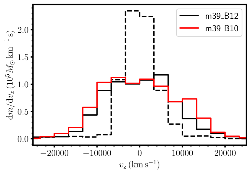
The lack of a clear bipolar structure can also be seen by considering the distribution of the iron-group material in velocity space. Figure 12 shows the distribution of the velocity component parallel to the rotation axis in the iron-group ejecta (which would be the line-of-sight velocity for an observer in the polar direction). In model m39_B12, the bulk of the iron-group material has velocities well below by the end of the simulation. Only minute amounts of iron-group material reach the large velocities well in excess of observed in hypernovae (Modjaz et al., 2016). Large ejecta velocities in m39_B10 are merely due to the shorter simulation time.
If these models were to be compatible with observed hypernovae, a more bipolar distribution of iron-group material would have to emerge later. It cannot be excluded that late-time mixing instabilities could redistribute the iron-group material appreciably, but at present it is not certainly not obvious that the magnetorotational explosions match the characteristics of observed hypernovae.
6 Gravitational Waves
6.1 Amplitudes and Spectrograms
For each of our models, the time series and spectrograms (evaluted using Matplotlib’s specgram function) of the GW emission are shown in Figure 13. We show distance-independent amplitudes for the plus polarisation mode, i.e., the product of strain of strain and observer distance . The cross polarisation amplitudes and spectrograms are very similar. At the pole, model m39_B12 reaches a maximum amplitude of 165 cm in the plus polarisation mode, and an amplitude of 152 cm in the cross polarisation. At the equator, the amplitudes are slightly smaller, namely 106 cm in the plus polarisation and 121 cm in the cross polarisation. For model m39_B10 model, the maximum amplitude at the pole is 133 cm in the plus polarisation and 152 cm in the cross polarisation. At the equator, this model also has smaller amplitudes, with 96 cm in the plus polarisation and 109 cm in the cross polarisation. Most of the detectable GW amplitudes occur within the first 400 ms and decrease significantly around the same time that the explosion energy starts to reach its final value.
These amplitudes are significantly higher than in the 2D simulations of these models in Jardine et al. (2022), which only reached amplitudes of 76 cm for m39_B10, and 62 cm for m39_B12 (disregarding the late-time tail signal). They found that model m39_B12 has a smaller GW amplitude than m39_B10 (which exploded late in 2D and hence had a longer phase of accretion-phase GW emission), which is the opposite of what we see in our 3D models. On the other hand, GW emission in m39_B12 tapers off more clearly at late times in our 3D simulation compared to the 2D model of Jardine et al. (2022). The GW amplitudes are also significantly larger than the maximum amplitudes of about in the non-magnetised model m39_B0, which is reflective of the more powerful explosions in the MHD models. Model m39_B12 develops a small tail in the plus polarisation only at the equator. Model m39_B10 also develops a very small tail, but it is visible at all observer directions. The tail also differs from the 2D case, as Jardine et al. (2022) show a significantly larger tail for model m39_B12 in 2D. The difference to the 2D case can be explained by the more modest bipolar deformation of the shock.
A dominant high-frequency emission band is clearly visible in the spectrograms of both models. It is evident somewhat more clearly than in the 2D counterpart of m39_B12 in Jardine et al. (2022) that the structure of the oscillation modes underlying GW emission is not qualitatively changed from the familiar picture in neutrino-driven CCSNe, where GW emission is predominantly due to the -mode or the -mode (Morozova et al., 2018; Torres-Forné et al., 2019; Sotani et al., 2021). The high-frequency band reaches up Hz by the end of the simulation in model m39_B12 and about 1,500 Hz in model m39_B10. The frequencies are higher than in our recent neutrino-driven simulations, which is due to the different treatment of gravity used in our MHD simulations; as noted by Müller et al. (2013) GW frequencies are systematically overestimated by in pseudo-Newtonian simulations due to the omission of metric terms in the equations of hydrodynamics.
Similar to Powell & Müller (2020), we do, however, find that the high-frequency emission band deviates quantitatively from the relations established for neutrino-driven supernovae of non-rotating progenitors. In the 2D case, Jardine et al. (2022) still found that the time dependence of the high-frequency f/g-mode emission band was well matched by the formula of Müller et al. (2013),
| (17) |
where is the radius of the PNS, is the electron antineutrino mean energy, is the neutron mass and is the baryonic mass of the PNS. As shown Figure 14, we find this relation does not match the high-frequency emission in 3D models. We also show the mode universal relation from Torres-Forné et al. (2019), which also does not match. The predicted frequencies are lower than what is observed in our models by Hz. The general shape of the time-dependence is somewhat similar, but there is clear quantitative mismatch. For m39_B12, the actual frequency trajectory has something more of an S-shape that bends up noticeably just before after bounce. As discussed in Powell & Müller (2020); Jardine et al. (2022), the impact of rotation and magnetic fields on PNS oscillation eigenfunctions and eigenfrequencies is not trivial and can just be stated as an empirical finding at this point. In future, linear eigenmode analysis (Torres-Forné et al., 2019; Sotani et al., 2021) will need to be extended to include rotation and magnetic fields to understand this effect. For now it remains important to consider that empirical scaling laws for the frequency of the dominant f/g-mode become uncertain in the presence of rapid rotation and magnetic fields and should be applied with care to prospective CCSN GW signals if rapid core rotation is determined from the bounce signal (Abdikamalov et al., 2014) or the observed explosion is very energetic and possibly magnetorotational in origin.
The emission frequency at the time of strongest emission is of critical importance for the prospects of detecting a CCSN in GWs. In Table 1, we therefore show the frequency at which the GW amplitude of the signal peaks. This peak frequency is between 1100 Hz and 1400 Hz for both models in different observer directions. We note that the peak frequencies, the overall width of the spectrum, and the time-frequency signal morphologies are very similar to the 2D case (Jardine et al., 2022). Importantly, this confirms that there is no significant amount of extra power above , which might accidentally be cut out by current choices of cut-off frequencies in event analysis (Abbott et al., 2020, 2021b).


6.2 Detection Prospects

In this section, we estimate the distances out to which our models could be detected by current and future GW detectors. In Table 1, we show the maximum detectable distances for each of our models for two different observer directions.
The maximum detectable distance is given by the distance needed for an optimal signal-to-noise ratio (SNR) of 8. The optimal SNR is defined as,
| (18) |
where is the frequency-domain GW signal, and is the GW detectors noise power spectral density (PSD). We give values for a single Advanced LIGO detector (LIGO Scientific Collaboration et al., 2015), Einstein Telescope (Hild et al., 2011) and Cosmic Explorer (Evans et al., 2021) detectors. The PSD curves we use for the different detectors are shown in Figure 15. We also determine the maximum detection distances for two different networks of detectors. The first is a network of LIGO, Virgo (Acernese et al., 2015) and KAGRA (Akutsu et al., 2021) detectors, and the second is a network of Cosmic Explorer detectors where the network SNR is defined as,
| (19) |
where and are the individual detector SNRs.
This method does not account for the short-duration transient noise artefacts found in real GW detector noise. We also do not account for the limitations of specific search algorithms. For example, Szczepańczyk et al. (2021), show that the current main morphology-independent search for GW bursts can detect CCSNe down to SNRs of . The core bounce and late time GW emission are not included in our GW models, which will also make the detection distances smaller than if we had full waveforms.
The detection distances for all our models are shown in Table 1. Model m39_B10 has the largest detection distances with up 260 kpc in a single LIGO detector, and up to 2.63 Mpc in a single Einstein Telescope detector. Note that model m39_B10 only covers half the simulation time of model m39_B12, so it is likely that the difference in detection distances would have grown if the models were continued for longer.
The detection distances are twice as large as those predicted for the same models in 2D in Jardine et al. (2022). This is partially due to the larger GW amplitudes in the 3D models and partially due to having both GW polarisation modes in 3D. As expected, the models have larger maximum detection distances than previous 3D simulations of non-rotating neutrino-driven explosions (Powell & Müller, 2019, 2020). There are no GW detection studies of long-duration 3D MHD models that we can compare to our results, but it should be noted that based on the post-bounce emission alone our models give comparable detection distance to MHD simulations of the core-bounce signal only (Abbott et al., 2020; Szczepańczyk et al., 2021). Different from the bounce signal, the detectability of the post-bounce signal does not depend significantly on the observer direction for our models and is therefore, in a sense, more robust. The pseudo-Newtonian gravity used in our simulations has likely increased the GW frequency by about 20%. This will have resulted in a decrease in the predicted detection distances, as the GW detectors have a better sensitivity at the lower frequencies.
| Model | Observer direction | LIGO | ET | CE | LVK | 2xCE | Frequency at peak | |||||
|---|---|---|---|---|---|---|---|---|---|---|---|---|
| name | (degrees of latitude) | distance | distance | distance | distance | distance | emission | |||||
| m39_B12 | 90 | 211 kpc | 2.15 Mpc | 3.66 Mpc | 331.6 kpc | 5.12 Mpc | 1395 Hz | |||||
| m39_B12 | 0 | 243 kpc | 2.40 Mpc | 4.11 Mpc | 375 kpc | 5.81 Mpc | 1159 Hz | |||||
| m39_B10 | 90 | 226 kpc | 2.34 Mpc | 3.96 Mpc | 358 kpc | 5.60 Mpc | 1288 Hz | |||||
| m39_B10 | 0 | 260 kpc | 2.63 Mpc | 4.47 Mpc | 405 kpc | 6.32 Mpc | 1337 Hz |
7 Conclusions
In this paper, we perform 3D MHD CCSNe simulations of two progenitor models with rapid rotation and two different initial magnetic field strengths of G and G. We also compare our results to our previous simulation of this progenitor model without magnetic fields.
Inclusion of strong magnetic fields resulted in shock revival by the magnetorotational mechanism, which occurred faster than our previous neutrino-driven explosion of this progenitor model with no magnetic fields. Both of the models show strong jets, which are, however, later affected by the kink instability. Model m39_B12 develops a jet ms after core bounce, but the jet in the North direction quickly disappears and only a jet in the South direction remains. The jets in model m39_B10 start a little later, but continues to grow larger in both directions up to the end of the simulation. Interestingly, the explosion is not primarily driven by the jets; the shock already expands more or less isotropically to about before fast jets start to emerge. Both models reach high explosion energies that level off only a few hundred milliseconds after the core-bounce. The explosion energy of about lies at the low end of the hypernova distribution.
Both of our new models have a significantly smaller final PNS mass than the m39_B0 model, with a final mass cut within the silicon shell of the progenitor. We do not observe any spin kick alignment in these models despite the alignment of the jets with the rotation axis. Importantly, the proto-neutron star is spun down on short time scales, so that its final rotation period is expected to be about . This would not leave enough rotational energy to launch a relativistic gamma-ray burst jet after the environment of the neutron star has been evacuated, but might still be sufficient to lead to a brightening of the light curve by energy input from pulsar spin-down.
The magnetorotational explosion models produce more than of iron-group material, which is superficially compatible with values inferred for observed hypernovae based on their light curves and spectroscopy. However, much of the iron-group material is not in the form of in our simulations since it is made by explosive burning of slightly neutron-rich material from the silicon shell. If one accepts the explosion dynamics of the models, the resulting nucleosynthesis should be relatively robust as it is not subject to uncertainties in the neutrino irradiation, unlike ejecta from close to the surface of the proto-neutron star. The iron-group material is also distributed quite isotropically by the end of the simulations. The bipolar distribution observed in hypernovae (Mazzali et al., 2001; Maeda et al., 2008; Tanaka et al., 2017) would have to emerge later by mixing instabilities.
We calculate the GW emission for our models. Both models have high amplitudes that are significantly larger than the non-magnetic model m39_B0. The GW signals reach high frequencies of over 1000 Hz. We show that our models do not fit previous relations for the GW frequency due to the magnetic fields and rapid rotation. The models could be detected up to a maximum distance of 260 kpc in Advanced LIGO and 4.47 Mpc in Cosmic Explorer.
While our models confirm that 3D magnetorotational explosion models are capable of reaching hypernova energies (Obergaulinger & Aloy, 2021b; Bugli et al., 2021), they clearly do not yet fit important characteristics of observed broad-lined Type Ic supernovae or magnetar-powered superluminous supernovae, and the newly born neutron star also rotates too slowly to enable a long-gamma ray burst in the millisecond magnetar scenario. They rather suggest that a scenario with a later onset of the explosion (due to weaker initial field or slow build-up of strong, large-scale magnetic fields after collapse) may be preferable over a rapid magnetorotational explosion scenario. Allowing longer accretion before a magnetorotational engine starts to operate, either within the millisecond magnetar or the collapsar scenario, would considerably increase the energy reservoir available for the explosion and might obviate the problem of inefficient nickel production. Clearly, two models for a single progenitor star are not sufficient to rule out the millisecond-magnetar scenario for hypernovae and long gamma-ray bursts. Nor can it be excluded that some rapid magnetorotational explosions of moderately high explosion energy are simply observed in a different guise and not as broad-lined Ic supernovae; e.g., it may worth scrutinising explosions with a high Ni/Fe ratio in the nebular phase more closely, as these could be explained by ejection of silicon-shell material (Jerkstrand et al., 2015a, b). At the very least our results suggest that requirements for plausible hypernova explosion models need to be investigated in greater detail. A wider exploration of stellar progenitor models (Obergaulinger & Aloy, 2022b) and initial field configurations (Bugli et al., 2021) may reveal a viable sweet spot for genuine hypernova explosions. Moreover, our results suggest that the evolution of magnetorotational explosions needs to be studied over longer time scales of seconds. The energetics of our models suggest the potential for fallback at later stages, which may still lead to the formation of a black hole and collapsar disk, or again spin up the PNS to trigger another “engine” phase that might further increase the explosion energy and launch a GRB jet. At any rate, fitting the various constraints on optical light curves and spectroscopy, gamma-ray and X-ray signatures, and nucleosynthesis constraints remains a formidable challenge that also requires a better connection between the short- and long-term evolution of magnetorotational explosions and the observational data.
Acknowledgements
Authors JP and BM are supported by the Australian Research Council (ARC) Centre of Excellence (CoE) for Gravitational Wave Discovery (OzGrav) project number CE170100004. JP is supported by the ARC Discovery Early Career Researcher Award (DECRA) project number DE210101050. BM is supported by ARC Future Fellowship FT160100035. We acknowledge computer time allocations from Astronomy Australia Limited’s ASTAC scheme, the National Computational Merit Allocation Scheme (NCMAS), and from an Australasian Leadership Computing Grant. Some of this work was performed on the Gadi supercomputer with the assistance of resources and services from the National Computational Infrastructure (NCI), which is supported by the Australian Government, and through support by an Australasian Leadership Computing Grant. Some of this work was performed on the OzSTAR national facility at Swinburne University of Technology. OzSTAR is funded by Swinburne University of Technology and the National Collaborative Research Infrastructure Strategy (NCRIS). D.R.A-D. acknowledges support by the Stavros Niarchos Foundation (SNF) and the Hellenic Foundation for Research and Innovation (H.F.R.I.) under the 2nd Call of “Science and Society” Action Always strive for excellence - “Theodoros Papazoglou” (Project Number: 01431).
Data Availability
The data from our simulations will be made available upon reasonable requests made to the authors.
References
- Abbott et al. (2019) Abbott B. P., et al., 2019, Physical Review X, 9, 031040
- Abbott et al. (2020) Abbott B. P., et al., 2020, Phys. Rev. D, 101, 084002
- Abbott et al. (2021a) Abbott R., et al., 2021a, Physical Review X, 11, 021053
- Abbott et al. (2021b) Abbott R., et al., 2021b, Phys. Rev. D, 104, 122004
- Abdikamalov et al. (2014) Abdikamalov E., Gossan S., DeMaio A. M., Ott C. D., 2014, Phys. Rev. D, 90, 044001
- Abdikamalov et al. (2020) Abdikamalov E., Pagliaroli G., Radice D., 2020, arXiv e-prints, p. arXiv:2010.04356
- Acernese et al. (2015) Acernese F., et al., 2015, Classical and Quantum Gravity, 32, 024001
- Aguilera-Dena et al. (2018) Aguilera-Dena D. R., Langer N., Moriya T. J., Schootemeijer A., 2018, ApJ, 858, 115
- Aguilera-Dena et al. (2020) Aguilera-Dena D. R., Langer N., Antoniadis J., Müller B., 2020, ApJ, 901, 114
- Akiyama et al. (2003) Akiyama S., Wheeler J. C., Meier D. L., Lichtenstadt I., 2003, ApJ, 584, 954
- Akutsu et al. (2021) Akutsu T., et al., 2021, Progress of Theoretical and Experimental Physics, 2021, 05A102
- Aloy & Obergaulinger (2020) Aloy M. Á., Obergaulinger M., 2020, Monthly Notices of the Royal Astronomical Society, 500, 4365
- Andresen et al. (2019) Andresen H., Müller E., Janka H. T., Summa A., Gill K., Zanolin M., 2019, MNRAS, 486, 2238
- Begelman (1998) Begelman M. C., 1998, ApJ, 493, 291
- Bisnovatyi-Kogan et al. (1976) Bisnovatyi-Kogan G. S., Popov I. P., Samokhin A. A., 1976, Ap&SS, 41, 287
- Blanchet et al. (1990) Blanchet L., Damour T., Schaefer G., 1990, MNRAS, 242, 289
- Blondin & Mezzacappa (2006) Blondin J. M., Mezzacappa A., 2006, ApJ, 642, 401
- Blondin et al. (2003) Blondin J. M., Mezzacappa A., DeMarino C., 2003, ApJ, 584, 971
- Bugli et al. (2020) Bugli M., Guilet J., Obergaulinger M., Cerdá-Durán P., Aloy M. A., 2020, MNRAS, 492, 58
- Bugli et al. (2021) Bugli M., Guilet J., Obergaulinger M., 2021, MNRAS, 507, 443
- Bugli et al. (2022) Bugli M., Guilet J., Foglizzo T., Obergaulinger M., 2022, arXiv e-prints, p. arXiv:2210.05012
- Buras et al. (2006a) Buras R., Rampp M., Janka H. T., Kifonidis K., 2006a, A&A, 447, 1049
- Buras et al. (2006b) Buras R., Janka H. T., Rampp M., Kifonidis K., 2006b, A&A, 457, 281
- Burrows & Vartanyan (2021) Burrows A., Vartanyan D., 2021, Nature, 589, 29
- Burrows et al. (2007) Burrows A., Dessart L., Livne E., Ott C. D., Murphy J., 2007, ApJ, 664, 416
- Chan et al. (2020) Chan C., Müller B., Heger A., 2020, MNRAS, 495, 3751
- Dedner et al. (2002) Dedner A., Kemm F., Kröner D., Munz C. D., Schnitzer T., Wesenberg M., 2002, Journal of Computational Physics, 175, 645
- Dimmelmeier et al. (2008) Dimmelmeier H., Ott C. D., Marek A., Janka H. T., 2008, Phys. Rev. D, 78, 064056
- Duncan & Thompson (1992) Duncan R. C., Thompson C., 1992, ApJ, 392, L9
- Edwards (2021) Edwards M. C., 2021, Phys. Rev. D, 103, 024025
- Eichler (1993) Eichler D., 1993, ApJ, 419, 111
- Ertl et al. (2020) Ertl T., Woosley S. E., Sukhbold T., Janka H. T., 2020, ApJ, 890, 51
- Evans et al. (2021) Evans M., et al., 2021, arXiv e-prints, p. arXiv:2109.09882
- Finn (1989) Finn L. S., 1989, in Evans C. R., Finn L. S., Hobill D. W., eds, Frontiers in Numerical Relativity. Cambridge University Press, Cambridge (UK), pp 126–145
- Finn & Evans (1990) Finn L. S., Evans C. R., 1990, ApJ, 351, 588
- Foglizzo et al. (2007) Foglizzo T., Galletti P., Scheck L., Janka H.-T., 2007, ApJ, 654, 1006
- Fuller et al. (2015) Fuller J., Klion H., Abdikamalov E., Ott C. D., 2015, MNRAS, 450, 414
- Gal-Yam (2017) Gal-Yam A., 2017, in Alsabti A. W., Murdin P., eds, , Handbook of Supernovae. p. 195, doi:10.1007/978-3-319-21846-5_35
- Gossan et al. (2016) Gossan S. E., Sutton P., Stuver A., Zanolin M., Gill K., Ott C. D., 2016, Phys. Rev. D, 93, 042002
- Grimmett et al. (2021a) Grimmett J. J., Müller B., Heger A., Banerjee P., Obergaulinger M., 2021a, MNRAS, 501, 2764
- Grimmett et al. (2021b) Grimmett J. J., Müller B., Heger A., Banerjee P., Obergaulinger M., 2021b, MNRAS, 501, 2764
- Gurski (2004) Gurski K. F., 2004, SIAM Journal on Scientific Computing
- Harris et al. (2017) Harris J. A., Hix W. R., Chertkow M. A., Lee C. T., Lentz E. J., Messer O. E. B., 2017, ApJ, 843, 2
- Hartmann et al. (1985) Hartmann D., Woosley S. E., El Eid M. F., 1985, ApJ, 297, 837
- Hild et al. (2011) Hild S., et al., 2011, Classical and Quantum Gravity, 28, 094013
- Iwamoto et al. (1998) Iwamoto K., et al., 1998, Nature, 395, 672
- Janka et al. (2022) Janka H.-T., Wongwathanarat A., Kramer M., 2022, ApJ, 926, 9
- Jardine et al. (2022) Jardine R., Powell J., Müller B., 2022, MNRAS, 510, 5535
- Jerkstrand et al. (2015a) Jerkstrand A., et al., 2015a, MNRAS, 448, 2482
- Jerkstrand et al. (2015b) Jerkstrand A., et al., 2015b, ApJ, 807, 110
- Johnston et al. (2005) Johnston S., Hobbs G., Vigeland S., Kramer M., Weisberg J. M., Lyne A. G., 2005, MNRAS, 364, 1397
- Kalogera et al. (2019) Kalogera V., et al., 2019, BAAS, 51, 239
- Kimura et al. (2013) Kimura M., Tsunemi H., Tomida H., Sugizaki M., Ueno S., Hanayama T., Yoshidome K., Sasaki M., 2013, PASJ, 65, 14
- Kobayashi et al. (2006) Kobayashi C., Umeda H., Nomoto K., Tominaga N., Ohkubo T., 2006, ApJ, 653, 1145
- Kruskal & Tuck (1958) Kruskal M., Tuck J. L., 1958, Proceedings of the Royal Society of London Series A, 245, 222
- Kuroda et al. (2014) Kuroda T., Takiwaki T., Kotake K., 2014, Phys. Rev. D, 89, 044011
- Kuroda et al. (2020) Kuroda T., Arcones A., Takiwaki T., Kotake K., 2020, ApJ, 896, 102
- LIGO Scientific Collaboration et al. (2015) LIGO Scientific Collaboration et al., 2015, Classical and Quantum Gravity, 32, 074001
- Lattimer & Schutz (2005) Lattimer J. M., Schutz B. F., 2005, ApJ, 629, 979
- Lattimer & Swesty (1991) Lattimer J. M., Swesty D. F., 1991, Nuclear Phys. A, 535, 331
- Lopez et al. (2013) Lopez L. A., Ramirez-Ruiz E., Castro D., Pearson S., 2013, ApJ, 764, 50
- MacFadyen & Woosley (1999) MacFadyen A. I., Woosley S. E., 1999, ApJ, 524, 262
- Maeda et al. (2002) Maeda K., Nakamura T., Nomoto K., Mazzali P. A., Patat F., Hachisu I., 2002, ApJ, 565, 405
- Maeda et al. (2008) Maeda K., et al., 2008, Science, 319, 1220
- Mazzali et al. (2001) Mazzali P. A., Nomoto K., Patat F., Maeda K., 2001, ApJ, 559, 1047
- Mazzali et al. (2007) Mazzali P. A., et al., 2007, ApJ, 670, 592
- Milisavljevic et al. (2015) Milisavljevic D., et al., 2015, ApJ, 799, 51
- Miyoshi & Kusano (2005) Miyoshi T., Kusano K., 2005, Journal of Computational Physics, 208, 315
- Modjaz et al. (2016) Modjaz M., Liu Y. Q., Bianco F. B., Graur O., 2016, ApJ, 832, 108
- Morozova et al. (2018) Morozova V., Radice D., Burrows A., Vartanyan D., 2018, ApJ, 861, 10
- Mösta et al. (2014) Mösta P., et al., 2014, ApJ, 785, L29
- Mösta et al. (2015) Mösta P., Ott C. D., Radice D., Roberts L. F., Schnetter E., Haas R., 2015, Nature, 528, 376
- Mösta et al. (2018) Mösta P., Roberts L. F., Halevi G., Ott C. D., Lippuner J., Haas R., Schnetter E., 2018, ApJ, 864, 171
- Müller (2020) Müller B., 2020, Living Reviews in Computational Astrophysics, 6, 3
- Müller & Janka (2014) Müller B., Janka H.-T., 2014, ApJ, 788, 82
- Müller & Janka (2015) Müller B., Janka H. T., 2015, MNRAS, 448, 2141
- Müller & Varma (2020) Müller B., Varma V., 2020, MNRAS, 498, L109
- Müller et al. (2008) Müller B., Dimmelmeier H., Müller E., 2008, A&A, 489, 301
- Müller et al. (2013) Müller B., Janka H.-T., Marek A., 2013, ApJ, 766, 43
- Müller et al. (2019) Müller B., et al., 2019, MNRAS, 484, 3307
- Müller et al. (2010) Müller B., Janka H.-T., Dimmelmeier H., 2010, The Astrophysical Journal Supplement Series, 189, 104
- Nakamura et al. (2001) Nakamura T., Mazzali P. A., Nomoto K., Iwamoto K., 2001, ApJ, 550, 991
- Ng & Romani (2007) Ng C.-Y., Romani R. W., 2007, ApJ, 660, 1357
- Nomoto et al. (2006) Nomoto K., Tominaga N., Umeda H., Kobayashi C., Maeda K., 2006, Nuclear Phys. A, 777, 424
- Noutsos et al. (2012) Noutsos A., Kramer M., Carr P., Johnston S., 2012, MNRAS, 423, 2736
- Noutsos et al. (2013) Noutsos A., Schnitzeler D. H. F. M., Keane E. F., Kramer M., Johnston S., 2013, MNRAS, 430, 2281
- O’Connor & Ott (2011) O’Connor E., Ott C. D., 2011, ApJ, 730, 70
- Obergaulinger & Aloy (2017) Obergaulinger M., Aloy M. Á., 2017, MNRAS, 469, L43
- Obergaulinger & Aloy (2020) Obergaulinger M., Aloy M. Á., 2020, MNRAS, 492, 4613
- Obergaulinger & Aloy (2021a) Obergaulinger M., Aloy M. Á., 2021a, MNRAS, 503, 4942
- Obergaulinger & Aloy (2021b) Obergaulinger M., Aloy M. Á., 2021b, MNRAS, 503, 4942
- Obergaulinger & Aloy (2022a) Obergaulinger M., Aloy M. Á., 2022a, MNRAS, 512, 2489
- Obergaulinger & Aloy (2022b) Obergaulinger M., Aloy M. Á., 2022b, MNRAS, 512, 2489
- Obergaulinger et al. (2006) Obergaulinger M., Aloy M. A., Müller E., 2006, A&A, 450, 1107
- Obergaulinger et al. (2014) Obergaulinger M., Janka H.-T., Aloy M. A., 2014, MNRAS, 445, 3169
- Pajkos et al. (2019) Pajkos M. A., Couch S. M., Pan K.-C., O’Connor E. P., 2019, ApJ, 878, 13
- Paxton et al. (2011) Paxton B., Bildsten L., Dotter A., Herwig F., Lesaffre P., Timmes F., 2011, ApJS, 192, 3
- Paxton et al. (2013) Paxton B., et al., 2013, ApJS, 208, 4
- Paxton et al. (2015) Paxton B., et al., 2015, ApJS, 220, 15
- Paxton et al. (2018) Paxton B., et al., 2018, ApJS, 234, 34
- Powell & Müller (2019) Powell J., Müller B., 2019, MNRAS, 487, 1178
- Powell & Müller (2020) Powell J., Müller B., 2020, MNRAS, 494, 4665
- Rampp & Janka (2002) Rampp M., Janka H. T., 2002, A&A, 396, 361
- Raynaud et al. (2022) Raynaud R., Cerdá-Durán P., Guilet J., 2022, MNRAS, 509, 3410
- Reichert et al. (2021) Reichert M., Obergaulinger M., Eichler M., Aloy M. Á., Arcones A., 2021, MNRAS,
- Reichert et al. (2022) Reichert M., Obergaulinger M., Aloy M. Á., Gabler M., Arcones A., Thielemann F. K., 2022, MNRAS,
- Richers et al. (2017) Richers S., Ott C. D., Abdikamalov E., O’Connor E., Sullivan C., 2017, Phys. Rev. D, 95, 063019
- Scheck et al. (2006) Scheck L., Kifonidis K., Janka H. T., Müller E., 2006, A&A, 457, 963
- Scheidegger et al. (2008) Scheidegger S., Fischer T., Whitehouse S. C., Liebendörfer M., 2008, A&A, 490, 231
- Shibagaki et al. (2020) Shibagaki S., Kuroda T., Kotake K., Takiwaki T., 2020, MNRAS, 493, L138
- Sieverding et al. (2020) Sieverding A., Müller B., Qian Y. Z., 2020, ApJ, 904, 163
- Sotani & Takiwaki (2016) Sotani H., Takiwaki T., 2016, Phys. Rev. D, 94, 044043
- Sotani et al. (2021) Sotani H., Takiwaki T., Togashi H., 2021, Phys. Rev. D, 104, 123009
- Stockinger et al. (2020) Stockinger G., et al., 2020, MNRAS, 496, 2039
- Suwa et al. (2007) Suwa Y., Takiwaki T., Kotake K., Sato K., 2007, PASJ, 59, 771
- Szczepańczyk et al. (2021) Szczepańczyk M. J., et al., 2021, Phys. Rev. D, 104, 102002
- Takahashi & Langer (2021) Takahashi K., Langer N., 2021, A&A, 646, A19
- Takiwaki & Kotake (2011) Takiwaki T., Kotake K., 2011, ApJ, 743, 30
- Tanaka et al. (2017) Tanaka M., Maeda K., Mazzali P. A., Kawabata K. S., Nomoto K., 2017, ApJ, 837, 105
- The LIGO Scientific Collaboration et al. (2021) The LIGO Scientific Collaboration et al., 2021, arXiv e-prints, p. arXiv:2111.03606
- Torres-Forné et al. (2018) Torres-Forné A., Cerdá-Durán P., Passamonti A., Font J. A., 2018, MNRAS, 474, 5272
- Torres-Forné et al. (2019) Torres-Forné A., Cerdá-Durán P., Obergaulinger M., Müller B., Font J. A., 2019, Phys. Rev. Lett., 123, 051102
- Usov (1992) Usov V. V., 1992, Nature, 357, 472
- Varma & Müller (2021) Varma V., Müller B., 2021, MNRAS, 504, 636
- Varma et al. (2021) Varma V., Müller B., Obergaulinger M., 2021, MNRAS, 508, 6033
- Varma et al. (2022) Varma V., Mueller B., Schneider F. R. N., 2022, arXiv e-prints, p. arXiv:2204.11009
- Wanajo et al. (2018) Wanajo S., Müller B., Janka H.-T., Heger A., 2018, ApJ, 852, 40
- Winteler et al. (2012) Winteler C., Käppeli R., Perego A., Arcones A., Vasset N., Nishimura N., Liebendörfer M., Thielemann F. K., 2012, ApJ, 750, L22
- Wongwathanarat et al. (2013) Wongwathanarat A., Janka H. T., Müller E., 2013, A&A, 552, A126
- Woosley (2010) Woosley S. E., 2010, ApJ, 719, L204
- Woosley & Bloom (2006) Woosley S. E., Bloom J. S., 2006, ARA&A, 44, 507
- Woosley et al. (1999) Woosley S. E., Eastman R. G., Schmidt B. P., 1999, ApJ, 516, 788