Three-$\alpha$ configurations of the second $J^{\pi}=2^{+}$ state in ¹²C

In this paper, the wave functions of ¹²C are described as a three-$\alpha$ system. The three-$\alpha$ Hamiltonian reads

where $T_{i}$ is the kinetic energy of the $i$th $\alpha$ particle. The kinetic energy of the center-of-mass motion $T_{\mathrm{cm}}$ is subtracted. The mass parameter in the kinetic energy terms and the elementary charge in the Coulomb potential $(V_{\rm Coul.})$ are taken as $\hbar^{2}/m_{\alpha}=10.654$ MeVfm² and $e^{2}=1.440$ MeVfm, respectively. Two-$\alpha$ interaction $V_{2\alpha}$ is taken as the same used in Ref. Fukatsu92 , which is derived by a folding procedure using an effective nucleon-nucleon interaction. We employ the three-$\alpha$ interaction $V_{3\alpha}$ depending on the total angular momentum $J^{\pi}$ reproducing the energies of the $0_{1}^{+}$ and $2_{1}^{+}$ states as was used in Ref. Ohtubo13 . Here we adopt the orthogonality condition model Saito68 ; Saito69 ; Saito77 . To impose the orthogonality condition to the Pauli forbidden states (f.s.), we introduce in the Hamiltonian the following pseudopotential Kukulin78 :

The summation of $nlm$ runs over all the f.s., i.e., $0S$, $1S$, and $0D$ states. We adopt the harmonic oscillator wave functions for $\phi_{nlm}$ with the size parameter $\nu=0.2575$ fm^-2 Fukatsu92 reproducing the size of the $\alpha$ particle. Taking $\gamma$ large enough, we exclude the Pauli forbidden states variationally from numerical calculations. In this paper, we take $\gamma=10^{5}$ MeV. The f.s. components of the resulting wave functions are found to be in the order of $10^{-5}$.

Denoting the $i$th single $\alpha$ particle coordinate vector by $\bm{r}_{i}$ $(i=1,2,3)$, we define a set of Jacobi coordinates $\bm{x}_{1}=\bm{r}_{2}-\bm{r}_{1}$ and $\bm{x}_{2}=\bm{r}_{3}-(\bm{r}_{1}+\bm{r}_{2})/2$, excluding the center-of-mass coordinate $\bm{x}_{3}=(\bm{r}_{1}+\bm{r}_{2}+\bm{r}_{3})/3$, which are denoted as $\tilde{\bm{x}}=(\bm{x}_{1},\bm{x}_{2})$, where a tilde stands for the transpose of a matrix. The $k$th state of the three-$\alpha$ wave function $\Psi_{JM}^{(k)}(\bm{x})$ with the total angular momentum $J$ and its projection $M$ is expressed in a superposition of fully symmetrized correlated Gaussian basis functions $G$ Varga95 ; SVMbook ,

where $\mathcal{S}$ is the symmetrizer which makes basis functions symmetrized under all particle-exchange, ensuring bosonic properties of $\alpha$ particles. A variational parameter $A_{i}$ is a 2 by 2 positive definite symmetric matrix, and $\tilde{\bm{x}}A\bm{x}$ is a short-hand notation of $\sum_{i,j=1}^{2}A_{ij}\bm{x}_{i}\cdot\bm{x}_{j}$. The angular part of the wave function is described by using the global vector $\tilde{u}\bm{x}=\sum_{j=1}^{2}u_{j}\bm{x}_{j}$ with $\tilde{u}=(u_{1},u_{2})$ and $u_{2}^{2}=1-u_{1}^{2}$ SVMbook ; Suzuki98 . A set of linear coefficients ${C_{i}^{(k)}}$ is determined by solving the generalized eigenvalue problem,

where the matrix elements $H_{ij}$ and $B_{ij}$ are defined as

The variational parameters $A_{i}$ and $u_{i}$ are determined by the stochastic variational method Varga95 ; SVMbook . For more details of the optimization procedure, the reader is referred to Refs.Phyu20 ; Moriya21 .

In this paper, we treat resonant $0_{2}^{+}$ and $2_{2}^{+}$ states as a bound state. This is the so-called bound-state approximation and works well for a state with a narrow decay width such as the $0_{2}^{+}$ state (Expt.: $\Gamma=8.5\times 10^{-3}$ MeV Ajzenberg90 ), while for the $2_{2}^{+}$ state it is hard to obtain the physical state with a simple basis expansion Funaki06 as it has somewhat a large decay width (Expt.: $\Gamma=1.01(15)$ MeV Itoh11 ). To estimate the resonant energy, the analytical continuation in the coupling constant ACCC is useful but does not provide us with the wave function. Nevertheless, a square-integrable wave function of a resonant state is useful to analyse its structure. A confining potential (CP) method Mitroy08 ; Mitroy13 is suitable for this purpose, as we can treat a resonance state as a bound state inside of the CP. To get a physical resonant state in the bound-state approximation, we introduce the CP in the following parabolic form Mitroy08 as

where $\Theta(r)$ is the Heaviside step function,

The strength $\lambda$ and range $R_{0}$ parameters of the CP are real numbers and have to be taken appropriately. Here we investigate the stability of the energies as well as the root-mean-square (rms) radii of $\alpha$ particles $R_{\rm rms}=\sqrt{\langle\Psi_{JM}|(\bm{r}_{1}-\bm{x}_{3})^{2}|\Psi_{JM}}\rangle$ of the $0_{1}^{+}$, $0_{2}^{+}$, $2_{1}^{+}$, and $2_{2}^{+}$ states against changes of $\lambda$ and $R_{0}$.

Figure 1 shows the energies and rms radii of the $0_{1}^{+}$, $0_{2}^{+}$, $2_{1}^{+}$ and $2_{2}^{+}$ states with different $R_{0}$. The strength of the confining potential is set to be $\lambda=100$ MeV/fm². Since the $R_{0}$ value is taken large enough, the energies and the rms radii of the bound states, the $0_{1}^{+}$ and $2_{1}^{+}$ states, do not depend much on these parameters. Even for the resonant $0_{2}^{+}$ and $2_{2}^{+}$ states, we find that the fluctuations of the energies are small about 0.1 MeV and 0.6 MeV, respectively, in the range of $R_{0}=8$–10 fm. This is reasonable considering the facts that the $0_{2}^{+}$ state has a quite small decay width and the $2_{2}^{+}$ state has a larger decay width. The magnitude of the radius fluctuation against the changes of $R_{0}$ is about $\approx 0.3$ fm for the $0_{2}^{+}$ state and $\approx 0.5$ fm for the $2^{+}_{2}$ state. We also made the same analysis by strengthening the strength $\lambda$ by 10 times and a similar plot was obtained. Hereafter, we use the results with $R_{0}=9$ fm, $\lambda=100$ MeV/fm².

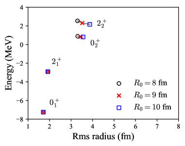
Table 1 lists the calculated energies and rms radii of $\alpha$ particles. These energy values can be compared with the real parts of the complex energies obtained by the complex scaling method (CSM) Ohtubo13 . The energies are 0.75 and 2.24 MeV for the $0^{+}_{2}$ and $2_{2}^{+}$ states, respectively, which are in good agreement with our results. Finally, we obtain the rms radii of the $0_{2}^{+}$ and $2_{2}^{+}$ states using these obtained wave functions. They are found to be similar and significantly large compared to the $0_{1}^{+}$ and $2_{1}^{+}$ states. For the sake of convenience, we also list the charge radii evaluated by $R_{\rm ch}=\sqrt{r_{\alpha}^{2}+R_{\rm rms}^{2}}$, where $r_{\alpha}$ is the charge radius of an $\alpha$ particle, 1.6755(28) fm Angeli13 . The calculated result for the ground state agrees with the theoretical result Kurokawa07 , showing reasonable reproduction of the measured charge-radius data 2.4702(22) fm Angeli13 . A large charge radius of the $0_{2}^{+}$ state is also consistent with that obtained in Ref. Kurokawa07 though its radius was given as a complex number.

To discuss the geometric configurations of the three-$\alpha$ systems, it is intuitive to see the two-body density distributions with respect to the two relative coordinates, $x_{1}$ and $x_{2}$, defined by

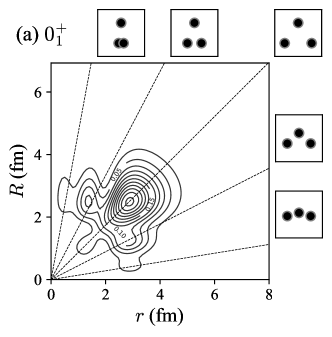
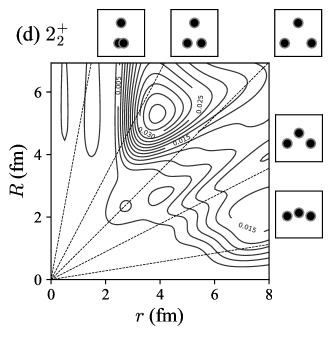
Note that the distribution is normalized as $\int_{0}^{\infty}dr\int_{0}^{\infty}dR\,\rho(r,R)=1$. Figure 2 plots the two-body density distributions of the $J^{\pi}=0_{1}^{+}$, $0_{2}^{+}$, $2_{1}^{+}$, and $2_{2}^{+}$ states. For a guide to the eyes, the specific $r/R$ ratios are indicated by the dashed lines and their corresponding geometric shapes are depicted by inset figures. We remark that the two-body density distributions were already discussed for the $J^{\pi}=0^{+}$ states in detail by using the shallow potential models Ishikawa14 ; Nguyen13 . Here we present the results with the OCM. The preliminary results for the $0^{+}$ states were already discussed in Ref. Moriya21FB but we repeat it to remind the characteristics of the two-body density distributions and to compare it with the $2^{+}$ state.

The two-body density distributions of the $0_{1}^{+}$ and $2_{1}^{+}$ states have similar peak structures; the most dominant peak is located on the equilateral triangle configuration at $r\sim$ 3 fm and some other peaks come from the nodal behavior of wave function due to the orthogonality of the forbidden states. We see different fine structures when a shallow potential model is employed. See Ref. Moriya21FB for detailed comparison.

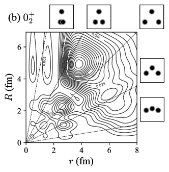
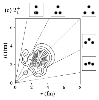
In contrast to the compact ground state, the two-body density distribution of the $0_{2}^{+}$ state is widely spreading. The most dominant peak of the $0_{2}^{+}$ state distribution is located at the acute-angled triangle configuration, which comes from the ${}^{8}{\rm Be}(0^{+})+\alpha$ structure Moriya21FB . For the $2_{2}^{+}$ state, likely to the $0_{2}^{+}$ state, the two-body density distribution spreads and the most dominant peak is located at the acute-angled triangle configuration. However, we find that the amplitude is significantly smaller than the $0^{+}_{2}$ state. The difference of these peak structures between the $0_{2}^{+}$ and $2_{2}^{+}$ states implies different intrinsic structure, which will be discussed in the next subsection.

At a closer look, we see the small peaks in the internal regions for the $0^{+}_{2}$ state, while they disappear for the $2_{2}^{+}$ state. This peak structure comes from the occupation of the nodal $S$ orbit but the occupation number in the $2_{2}^{+}$ state is much smaller than that of the $0_{2}^{+}$ state Yamada05 . Because the $2_{1}^{+}$ state already has a large occupation number of the $S$ orbit, there is no space to accommodate the nodal $S$ orbit in the $2_{2}^{+}$ state which should be orthogonal to the $2_{1}^{+}$ state.

In this subsection, we discuss more detailed structure of these three-$\alpha$ wave functions. For this purpose it is convenient to calculate the partial-wave component and ⁸Be spectroscopic factor, which are respectively defined by

where $\phi_{l}$ is the radial wave functions of ${}^{8}\mathrm{Be}$ with the relative angular momentum $l=0,2$, or 4, which correspond to physical resonant states with $J^{\pi}=0^{+},2^{+}$ or $4^{+}$, respectively, obtained by solving the two-$\alpha$ system using the same two-$\alpha$ potential adopted in this paper. The CP is also applied to evaluate these resonant states, and hence the obtained wave functions are square-integrable. The $P_{l_{1}l_{2}}$ value is the probability of finding $(l_{1},l_{2})$ component in the three-$\alpha$ wave function, while the $S_{l_{1}l_{2}}$ value can be a measure of the the ${}^{8}{\rm Be}+\alpha$ clustering. Note that given $l_{1}$ and $l_{2}$, $S_{l_{1}l_{2}}$ is a subspace of $P_{l_{1}l_{2}}$, hence $S_{l_{1}l_{2}}\leq P_{l_{1}l_{2}}$ always holds.

Table 2 lists the $P_{l_{1}l_{2}}$ and $S_{l_{1}l_{2}}$ values for the $0^{+}$ and $2^{+}$ states. The $0_{1}^{+}$ state has almost equal $P_{l_{1}l_{2}}$ values for $l_{1}=l_{2}=0,2$, and 4, which can be explained by reminding that the state has the SU(3)-like character Yamada05 . The higher partial-wave components is found to be $\approx 1$%. The $0^{+}_{1}$ wave function has about 50% of the ${}^{8}{\rm Be}+\alpha$ component. The $2^{+}_{1}$ state is mainly composed of $(l_{1},l_{2})=(2,2)$ and (4,4) components, $P_{22}$ and $P_{44}$, reflecting SU(3) character as like the $0_{1}^{+}$ state Yamada05 and also contains about half of the ${}^{8}{\rm Be}+\alpha$ component. Consequently, the structure of the $2_{1}^{+}$ state can be interpreted as a rigid rotational excited state of the $0_{1}^{+}$ while keeping its geometric shape as was shown in Fig. 2.

On contrary, the $P_{l_{1}l_{2}}$ values of $0_{2}^{+}$ concentrate only on the $l_{1}=l_{2}=0$ channel about 80%, which is consistent with the microscopic cluster model calculations Matsumura04 ; Yamada05 . This characteristic behavior is often interpreted as the bosonic condensate state of the three-$\alpha$ particles Tohsaki01 ; Yamada05 . This $(l_{1},l_{2})=(0,0)$ channel mostly consists of the ${}^{8}{\rm Be}(0^{+})+\alpha$ component shown in Table 2, forming the acute-angled triangle shape in the two-body density distribution Moriya21FB .

For the $2_{2}^{+}$ state, dominant partial-wave components are the $(l_{1},l_{2})=(0,2)$ and (2,0) channels. The ${}^{8}{\rm Be}(0^{+})+\alpha$ component is dominant in the $(l_{1},l_{2})=(0,2)$ channel, while few ${}^{8}{\rm Be}(2^{+})+\alpha$ component is found in the $(l_{1},l_{2})=(2,0)$ channel, which is in contrast to the $0_{2}^{+}$ state mainly consisting of the ${}^{8}{\rm Be}+\alpha$ configuration. This strong suppression can naturally be understood by considering the fact that the excitation energy of ${}^{8}\mathrm{Be}(2^{+})$ is rather high 3.26 MeV (Expt.: 3.12 MeV Tilley04 ), compared to the calculated energy spacing between the $0_{2}^{+}$ and $2_{2}^{+}$ states, $\approx 1.4$ MeV. This suggests that the $2_{2}^{+}$ state is not a simple rigid rotational excited state of the $0_{2}^{+}$ state but a partially rotational state. We remark that this interpretation supports the mean-field-like picture: The three $\alpha$ particles occupy the same $S$ state in the $0_{2}^{+}$ state Tohsaki01 , while one $S$-state $\alpha$ particle is excited to the $D$ state in the $2_{2}^{+}$ state Yamada05 . Such a $D$-wave excitation is possible with lower energy than the ⁸Be excitation if the frequency of the mean-field potential is low enough.

To discuss the role of the dominant channels in the geometric configurations in the $0_{2}^{+}$ and $2_{2}^{+}$ states, it is useful to evaluate the ⁸Be spectroscopic amplitude (SA)

Note that $\int_{0}^{\infty}dR\,[R\theta_{l_{1}l_{2}}(R)]^{2}=S_{l_{1}l_{2}}$. For practical calculations, see Appendix A of Ref. Suzuki09 , where an explicit formula of the SA with the correlated Gaussian basis function was given.

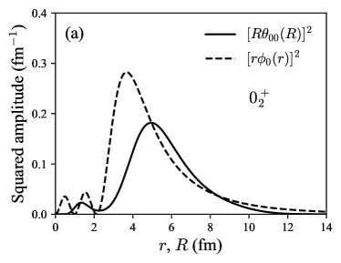
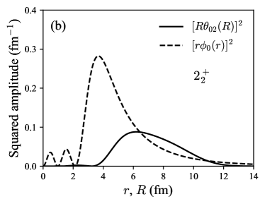
Figure 3 shows the SA with $(l_{1},l_{2})=(0,0)$ for the $0_{2}^{+}$ state and (0,2) for the $2_{2}^{+}$ state, which respectively correspond to the dominant configurations for each state. The SA of the $2^{+}_{2}$ state is smaller than that of the $0^{+}_{2}$ state reflecting the magnitudes of the $S_{l_{1}l_{2}}$ values. For the sake of comparison, we also plot the radial wave function of ⁸Be($0^{+}$), $\phi_{0}(r)$. The peak position of $r\phi_{0}(r)$ is located at 3.68 fm, while the SA has the largest peak at 4.97 fm for the $0_{2}^{+}$ state and 6.20 fm for the $2_{2}^{+}$ state. Though the latter distribution is broad, these are consistent with the fact that the highest peak of the two-body density distribution is located at $(r,R)=(3.9,5.1)$ fm for the $0_{2}^{+}$ state and $(r,R)=(3.9,5.3)$ fm for the $2_{2}^{+}$ state, exhibiting the acute-angled triangle configuration as shown in Fig. 2.

We also evaluate the rms radii of the SA defined by $D_{l_{1}l_{2}}=\sqrt{\int_{0}^{\infty}dR\,R^{2}[R\theta_{l_{1}l_{2}}(R)]^{2}/S_{l_{1}l_{2}}}$, listed in Table 2. The SA radii of the dominant channel of the $0_{2}^{+}$ and $2_{2}^{+}$ states are 5.84 fm with $(l_{1},l_{2})=(0,0)$ and 7.38 fm with $(l_{1},l_{2})=(0,2)$, respectively. Since the rms distance of the ⁸Be wave function is 5.32 fm, the ${}^{8}{\rm Be}+\alpha$ configuration induces an acute-angled triangle geometry.