Thermodynamics of non-linearly charged Anti-de Sitter black holes in four-dimensional Critical Gravity
Abstract
In this work, we provide new examples of Anti-de Sitter black holes with a planar base manifold in four-dimensional Critical Gravity by considering nonlinear electrodynamics as a matter source. We find a general solution characterized by the presence of only one integration constant where, for a suitable choice of coupling constants, we can show the existence of one or more horizons. Additionally, we compute its nonzero thermodynamical quantities through a variety of techniques, testing the validity of the first law of thermodynamics as well as a Smarr formula. Finally, we analyze the local thermodynamical stability of the solutions. To our knowledge, these charged configurations are the first example with Critical Gravity where their thermodynamical quantities are not zero.
I Introduction
Since its introduction in the late nineties, the idea of the Anti-de Sitter / Conformal Field Theory (AdS/CFT) correspondence [1] has gained momentum in different areas due to its potential to shed light on phenomena that range from superconductivity to quantum computing. This correspondence has also generated the need for the study of theories other than General Relativity due to two main reasons: first, the necessity to have theories that exhibit desired symmetries and properties that match the non-relativistic systems in the context of the correspondence and, secondly, the possibility that these enhanced theories may support a variety of thermodynamically rich AdS black holes, whose holographic role will be to introduce the non-relativistic behavior at finite temperature.
In this context, quadratic curvature gravities have been very successful in providing a plethora of new black hole configurations [2, 3, 4, 5, 6, 7]. A notable example within these theories in 2+1 dimensions is New Massive Gravity [8], a parity-even, renormalisable theory that, at the linearized level, is equivalent to the unitary Fierz-Pauli theory for free massive spin-2 gravitons, where AdS solutions have been previously found [9, 10]. A four-dimensional analogue to this theory is Critical Gravity (CG) [11], which is a ghost-free, renormalizable theory of gravity with quadratic corrections in the curvature111In general, a theory with quadratic corrections in curvature will propagate massive scalar and spin-2 ghost fields. In CG, the relation between the coupling constants and the cosmological constant leads to a theory in which the scalar field is zero and the spin-2 field becomes massless and with vanishing energy. . A particularity of CG is that its vacuum admits an AdS black hole solution given by
| (1) | |||||
where is an integration constant. However, as emphasized by the authors in [11], this solution is massless and has a vanishing entropy. This is also highlighted in [12, 13] in four and six dimensions, where the entropy, as well as global conserved charges of their black holes solutions, vanish identically.
Because of the interest of obtaining black hole solutions that can be framed in the context of the gauge/gravity correspondence, in this work we aim to find new AdS black hole configurations that can be supported by CG and exhibit non-vanishing thermodynamical properties. To achieve this, a nonlinear electrodynamics (NLE) source is employed [14]. The origin of NLE dates to , the year in which Mie G. explored this formalism for the first time [15]. Some years later, in the thirties, and motivated in part to avoid the well-known singularity of the field of a point particle, Born and Infeld [16, 17, 18] proposed new research , giving rise to the Born-Infeld (BI) theory [19, 20, 21]. Given the complexity to carry out an extension of BI towards solutions of nonlinear equations, this formalism had a stage of stagnation for almost three decades. Nevertheless, around the sixties, J. F. Plebánski presented an outstanding work for NLE in a medium, in which the theory is developed through an antisymmetric conjugate tensor (known as of Plebánski tensor) and a structure-function , where and are the invariants that are formed with the antisymmetric conjugate Plebánski tensor. Here, the structure-function is associated with the Lagrangian function , that depends on the invariants quadratics constructed from the Maxwell tensor , which can be determined by a Legendre transformation. At the end of the eighties, H. Salazar, A. García, and J. Plebánski found solutions for the equations of NLE coupled to gravity using the formalism [14], in which the BI theory appears as a special case [22]. Some of the benefits provided by the Plebánski formalism is the ability to obtain regular black hole solutions [23, 24, 25, 26, 27], Lifshitz black hole configurations that exist for any value of the dynamic exponent [28], and recently an exact solution of a massive, electrically and magnetically charged, rotating stationary black hole has been found [29, 30, 31]. In General Relativity, NLE has been a valuable tool in order to build exact black hole configurations, some of which exhibit non-standard asymptotic behavior in Einstein’s gravity or in its generalizations, as can be verified in [32, 33, 34, 35, 36, 37, 38]. It is relevant to mention that, in these works, charged black hole solutions that come from nonlinear theories possess interesting thermodynamic properties [39, 40, 41, 42, 43, 44]. All the above shows NLE as an interesting and motivating study field that we aim to explore with the addition of CG. As such, our action of interest will be given by:
| (2) |
with
where is the cosmological constant. As stated above, CG allows for the massive spin- field to vanish if the coupling constants and are restricted to obey the relations
| (3) |
Moreover, the Lagrangian density describes the nonlinear behavior of the electromagnetic field with field strength . The introduction of , which is an antisymmetric secondary field function of the original field , arises from the need to establish a relationship between standard electromagnetic theory with Maxwell’s theory of continuous media.
The source, described by the structure function is, of course, real and depends on the invariant formed with the conjugated antisymmetric tensor , which is , . In general, the structural function also depends on the other invariant where ∗ represents the Hodge dual. Here, this invariant is zero because we are interested in static configurations.
The field equations that result from the variation of the action (2) are
| (4a) | |||||
| (4b) | |||||
| (4c) | |||||
| where the tensors and are defined as follows: | |||||
with and given previously in (3). Note that equation (4a) represents the nonlinear version of Maxwell’s equations, while the constitutive relations are encoded in (4b) and Einstein’s equations are given by (4c).
These equations of motion (4a)-(4c) will lead us to find new AdS black hole configurations in CG coupled with non-linear electrodynamics in section II. Then, in section III, we will show the analysis and characterization of said solutions in terms of the maximum number of horizons. In section IV, the thermodynamical quantities and local stability of the solutions are calculated, and the first law of thermodynamics as well as the Smarr formula are verified. Finally, in section V we present our conclusions and perspectives of this work.
II Solution to the Equations of motion
We start the search of new AdS black hole solutions by considering the following asymptotically AdS metric ansatz
| (5) |
where , the planar coordinates both are assumed belong to a compact set, this is and , and the gravitational potential must satisfy the asymptotic condition
In our case, we propose the structure function , determining the nonlinear electrodynamics, to be given by
| (6) | |||||
where , and are coupling constants.
For the purposes of this article, we consider purely electrical configurations, such that . If we replace the previous ansatz in the nonlinear Maxwell equation (4a) we obtain
| (7) |
Therefore, the electric invariant is negative definite, since we only consider purely electrical configurations, which reads
| (8) |
where is a constant of integration related to the electric charge, and from (6) is a real function. The electric field is obtained from the constitutive relations (4b), . Using expression (6) for , the electromagnetic field strength results in
| (9) |
Notice that in order to recover the AdS spacetime asymptotically, the cosmological constant must take the following value,
| (10) |
Let us bring our attention to the fact that the difference between the temporal and radial diagonal components of the mixed version of Einstein’s equations (4c) is proportional to the following fourth-order Cauchy-Euler ordinary differential equation
| (11) |
Therefore, the solution of the gravitational potential is
| (12) |
where the fourth integration constant is fixed to comply with the asymptotic behaviour . Additionally, if we replace the expressions in (12) and (8) in the equations of motion (4c) we obtain an equation to determine , which can be later integrated to obtain , given previously in (6). Finally, the remaining equations of motion are satisfied if the previous integration constants ’s from (12) are fixed in terms of the charge-like parameter through the structural coupling constants as follows
| (13) |
where the ’s are in the appropriate units in order to the integration constants ’s be dimensionless. The addition of the NLE yields to a rich structure for the metric function obtained previously in (12)-(13), where the uncharged case is recovered when . This also shows that the linear Maxwell field scenario (that is ) is not allowed, which reinforces the necessity to explore other charged theories such as NLE. Moreover, from a physical perspective, this new structure for the metric function constructed via CG and NLE (2), will allow us to explore solutions with different numbers of horizons, in addition to nonzero thermodynamic quantities, as we will see bellow. These solutions are, to our knowledge, the first example of solutions in four-dimensional CG where their thermodynamic parameters do not vanish.
III Analysis of the solutions
We have established that the introduction of non-linear electrodynamics when considering CG, results in AdS solutions of the form (5) where
| (14) |
provided that and are given by (6) and (10) respectively. However, this set of expressions only represents a black hole solution if a horizon can be formed, that is, if there exists such that .
To this effect, in the following subsections, we study the conditions in which eq. (14) can vanish, through the analysis of its asymptotic behavior as well as its maxima and minima.
First, let us notice that when , will approach 1 asymptotically and, in this regime, . As a result, the sign of will determine whether the function approaches the horizontal asymptote from above or from below. Next, let us observe that when , , that is, the sign of will determine if the function starts increasing from or decreasing from in the region .
Moreover, we can perform an analysis of the extreme values of . From the calculation of we find that admits two extreme values which are located at
| (15) |
where the nature of these extreme values (whether they are a maximum or a minimum) will depend on the sign of their evaluation in , that is
| (16) |
with . Here, (resp. ) is associated with positive (resp. negative) sign in equations (15) and (16). Let us notice that from eqns. (15)-(16), the existence of real extreme values is limited to the fulfillment of the condition
| (17) |
At this point, we are ready to analyze each case independently.
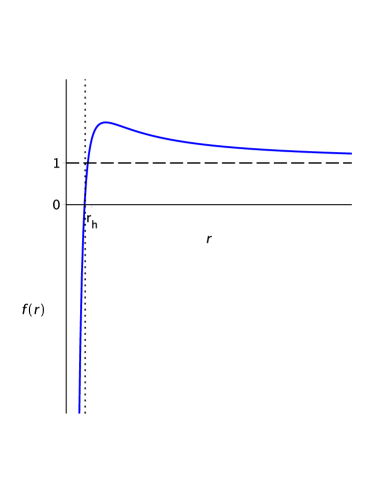
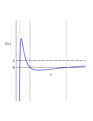
III.1 Black holes with one horizon: The case and
As previously mentioned, one can start by analyzing the asymptotical behavior of the function in eq. (14). If one considers the limit , the dominating term of is . Assuming and , then it is clear to see that for , . On the other hand, if we analyze the regime , we note that, in this limit, the dominant term of is which shows that, as increases, the function will asymptotically approach a horizontal asymptote . In short, for the case , considering only positive values for , the function starts in the fourth quadrant and it increases for small values of , since the function asymptotically approaches the value of as approaches infinity, it must cross the horizontal axis, ensuring the existence of an event horizon . Moreover, if we consider , the function will asymptotically approach the horizontal asymptote from above. Also, after analyzing the first and second derivatives of , we note that the choice for the sign of and will result in the function displaying an absolute maximum in the regime , and the existence of a single horizon, regardless of the sign of , as seen in Fig. 1. This analysis is deeply studied in the Appendix A.1.
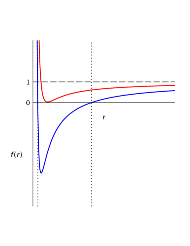
III.2 Black holes with up to two horizons: The case
On the contrary, when , the gravitational potential is initially decreasing in the region , one can face three scenarios: having two horizons, the extremal case of one horizon, or no horizon at all, which does not represent a black hole. Landing on one case or another depends on the relations between , and . Eq.(14) will represent the gravitational potential of a black hole only provided that
| (18) |
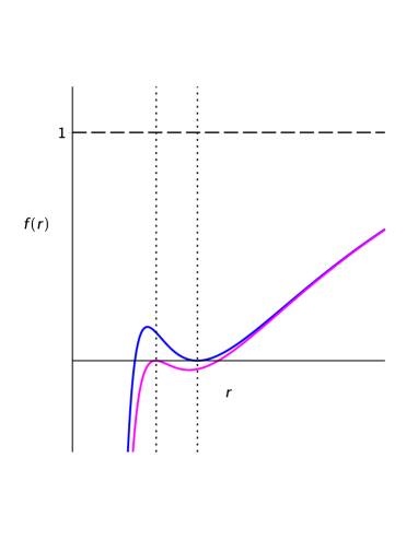
When the strict inequality is met, the solution will have two horizons (where the minimum is situated at ). Otherwise, when the equality is met, the solution will correspond to an extremal configuration, in which the minimum of is located at . Moreover, according to eqn. (16), when , the function will showcase a minimum; on the other hand, when , the function will have both a minimum and a maximum, as seen in Fig. 2. This study is analyzed in Appendix A.2.
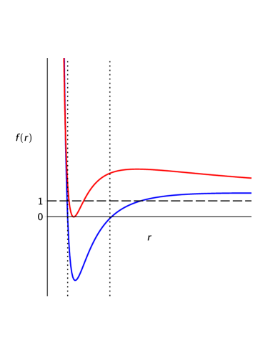
III.3 Black holes with up to three horizons: The case and
Finally, when we consider the case and . For very small but positive values of , we notice that the function is increasing from while, for large values of (that is ), the function approaches the value of 1 from below. This ensures the existence of at least one horizon (in the region ). However, under certain circumstances we observe that this case can admit up to three horizons, exhibiting one maximum and one minimum in the region . The conditions that will determine which case we will land in are detailed in the Appendix, but let us now state, in advance, that when the conditions , , and are met, we will have a solution with three horizons. In Fig. 3, we show examples of both cases for clarity. However, it is interesting to remark that, this case also admits two horizons when the maximum corresponds to the internal horizon or when the minimum corresponds with the outer horizon, as seen in Fig. 5. This scenario is fully explored in the Appendix A.3.
IV Thermodynamics and local stability of the solution
Given the structure of these new nonlinearly charged black hole solutions in four dimensions, it is interesting to explore their thermodynamics. As a first step, we will consider the electric charge which reads
| (19) |
where is the location of the event (or outer) horizon which can be expressed as , where is a root of the cubic polynomial
| (20) |
is the finite volume of the compact planar base manifold given by , while and are the unit spacelike and timelike normals to a sphere of radius given by
| (21) |
As a first step to calculate the electric potential we must determine the 4-potential . We achieve this by integrating eq. (II) and taking into account that . As a result the only non-zero component of the 4-potential is given by
| (22) |
where the integration constant in our case is null, and the electric potential 222In this work we have used the same definition of the electric potential as [42, 43, 44]. is given by:
| (23) | |||||
On the other hand, to compute the entropy we will consider Wald’s formula [45, 46] which, in our case, yields to
| (24) | |||||
where
with and subject to (3), and the integral is evaluated on a 2-dimensional spacelike surface (the bifurcation surface) characterized by the fact that the timelike Killing vector vanishes, denotes the determinant of the induced metric on , represents the binormal antisymmetric tensor constructed via the wedge product of the unit normal vectors and from (21), normalized as . Additionally, the Hawking temperature takes the form
| (25) | |||||
where is the surface gravity which reads
Finally, to calculate the mass of these charged AdS black hole configurations we will consider the approach described in [47, 48], corresponding to an off-shell prescription of the Abbott-Desser-Tekin (ADT) procedure [49, 50, 51]. The choice of this method to calculate conserved charges is ideal for CG due to the presence of quadratic curvature terms in its gravitational action.
The main elements of the quasilocal method are the surface term
| (26) | |||||
and the Noether potential
| (27) | |||||
With all the above, using a parameter , we interpolate between the charged solution at and the asymptotic one at , resulting in the quasilocal charge:
where is the difference of the Noether potential between the interpolated solutions. For this particular case the mass reads
| (28) |
Notice that for the Wald entropy (24), as well as the mass (28), the presence of the coupling constants and is providential, reinforcing the importance of the non-linear electrodynamic as a matter source with this gravity theory. In fact, when , the vector potential (22) vanishes, recovering the well known four-dimensional Schwarzschild- AdS black hole with a planar base manifold in CG, whose extensive thermodynamical quantities and are null, while the Hawking Temperature is .
Just for completeness, from eqns. (28), (24) and (19) we have:
and together with the electric potencial (23) as well as the Hawking temperature (25), a first law of the black holes thermodynamics
| (29) |
arises. Together with the above, through the thermodynamical parameters (19), (23)-(25), we can express the mass (28) as a function of the extensive thermodynamical quantities and in the following form
| (30) | |||||
with
| (31) |
where it is straightforward to verify that the intensive parameters
are consistent with the expressions (23) and (25) (where the subindices stand for at constant electric charge , and at constant entropy respectively). Additionally, under a rescaling with a nonzero parameter , equation (30) becomes
yielding to a four-dimensional Smarr formula [52]
| (32) |
which corresponds to a particular case of the higher-dimensional situation [40]
| (33) |
where is the dimension of the space-time, highly explored in [53, 54, 55].
Given these thermodynamical quantities, it is interesting to study this system under small perturbations around the equilibrium. In our case, we will consider the grand canonical ensemble, where the intensive thermodynamical quantities are fixed. With this, we can express the entropy, mass, and charge in functions of and in the following form
| (34) | |||||
| (35) | |||||
| (36) | |||||
With this information, we are in a position to determine the local thermodynamical (in)stability of this charged black hole solution under thermal fluctuations through the behavior of the specific heat , given by
| (37) | |||||
Here we observe that for or in the same way,
| (38) |
the specific heat becomes non-negative when
| (39) |
which can be interpreted as a locally stable configuration. Nevertheless, it is worth pointing out that, to have a real and well-defined mass according to the expression (30) as well as specific heat (37), only the strict inequalities from (38) and (39) are considered . Therefore, here we can conclude that the introduction of the nonlinear electrodynamics to the CG action induces rich thermodynamical properties. The comment on stability above is consistent with the analysis of the Gibbs Free Energy , given by
where its Hessian matrix , with , satisfies the conditions
| (41) |
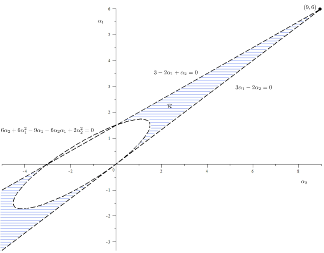
hold, where was defined previously in (31) and in order to have a well-defined Gibbs free energy (IV), we consider only the strict inequality from (41). As an example, for , which implies that , we have that the strict inequalities (38)-(39) and (41) are satisfied when the constants and belong to the region represented in the Figure 4.
Additionally, it is interesting to note that for this new charged black hole, we can analyze its response under electrical fluctuations, represented by the electric permittivity at a constant temperature, which reads as follow:
which is a non-negative quantity if the strict inequality (41) holds, ensuring local stability [39, 56].
V Conclusions and discussions
In this work we propose a nonlinear electrodynamics in the -formalism, which allows us to obtain charged configurations of AdS black holes in four dimensions with a planar base manifold in CG. These configurations have only one integration constant, given by the charge-like parameter , and being parameterized by the structural coupling constants (13). As was explained at the beginning, to our knowledge, these planar configurations are the first example of solutions in four-dimensional CG where their thermodynamic quantities do not vanish.
With respect to the metric function, the structural coupling constants play a very important role in the characterization of these charged solutions and when analyzing condition (17), we conclude that there are five different cases: one represents a black hole with three horizons, two cases represent black holes with two horizons and the other two are single horizon configurations.
Also, in order to find these new charged black holes, the introduction of nonlinear electrodynamics to CG allows us to obtain nonzero thermodynamic properties, thanks to the contributions given by and . Together with the above, these configurations satisfy the four dimensional Smarr relation (32) as well as the First Law (29). Additionally, the Critical-Gravity-non-linear electrodynamics model enjoys local stability under thermal fluctuations, thanks to the non-negativity of the specific heat as well as the Gibbs Free Energy analysis if (38)-(39) and (41) are satisfied. Supplementing the above, the non-negativity of the electric permittivity shows that our solution is also a locally stable thermodynamic system under electrical fluctuations. It is interesting to note the behavior of for these charged configurations, as it is a non-negativity quantity if , unlike other solutions found in the literature (see for example [54]).
Some natural extensions of this work may include, the exploration of other gravity theories with quadratic contributions. In this sense, a theory that also showcases critical conditions, is given in [57] where the square of the Weyl tensor and the square of the Ricci scalar play the main roles in the action, in the absence of the Einstein Gravity. Another interesting scenario would be to study the higher dimensional case [58], where now the CG Lagrangian takes the form
and that the coupling constants are tied as [59]
where the four dimensional case (2)-(3) can be recovered impossing together with the transformation
Given the power of the non-linear electrodynamics as a matter source to find new solutions with a planar base manifold, it would be interesting to study charged black holes where their event horizons enjoy spherical or hyperbolical topologies. It would also be interesting to study charged black hole configurations with non-standard asymptotically behaviors, such as Lifshitz black holes, which were first explored for the uncharged case with CG in [60]. For spherically symmetric metrics, it is possible, as was shown in [61], to obtain a generalization of the Smarr relation as well as the first law of black hole mechanics, being understood from a dual holographic point of view and related to the black hole chemistry [62, 63, 64], where now the cosmological constant takes the role as a dynamical variable, unlike the expression found in (32) where we explored charged planar black holes and does not appear in an active way.
Finally, from a physical motivation, these nonzero extensive thermodynamical quantities will allow us to explore, from a holographic point of view, the connection between black holes and quantum complexity [65, 66], as well as the effects on shear viscosity [67, 68, 69], where the mass and the entropy take a providential role.
Acknowledgments
The authors would like to thank Daniel Higuita, Julio Méndez, Eloy Ayón-Beato and Julio Oliva for useful discussion and comments on this work. The authors thank the Referee for the commentaries and suggestions to improve the paper.
Appendix A Analysis of extrema of the black hole solutions
In this work, we find that CG admits black hole solutions provided the existence of a non-linear electrodynamics described by eq. (6), and that these solutions are characterized by the gravitational potential (14), where, in our context, . However, the nature of these solutions and, in particular, the number of horizons that they will exhibit, will depend on the signs and relations between the constants ’s. In this appendix, we make an analysis of the extrema of the function to give a general classification of the solutions. Let us recall, from expression (15), that the existence of extreme values is limited to the fulfillment of the condition (17). Let us notice that when and have opposite signs, the condition above is met immediately, regardless of the value or sign of . That is, the existence of extreme values is assured. Let us then, start by analyzing both cases in detail.
A.1 Case
Upon inspecting eqn. (16) when considering , we notice that corresponds to a minimum and corresponds to a maximum. Moreover, from (15) , we notice that for these values of and , the maximum will always be on the interval (while the minimum will be in the region ). Combining this information with the asymptotical behavior of , we can conclude that for the case , the black hole will always have one horizon, as seen in Figure 1.
A.2 Case
Likewise, the condition (17) is always met when and , regardless of the sign of . This means that, in this case too, there will always be extreme values. Again, studying the second derivative of evaluated in the extreme values (see eqn. (16)), we notice that and correspond to a minimum and a maximum respectively, and that for these values of , the minimum will always be on the interval and the maximum in the region (under our analysis, we suppose that ). If we additionally consider the asymptotical behavior of (which states that will be decreasing for small positive values of ), we find that for this case the black hole will have a minimum. This means that can display up to two horizons, as seen in Figure 2 Top black curve.
For this solution to display both horizons, the strict inequality in (18) must be met, while the strict equality would correspond to the extremal black hole (Figure 2 Top red curve). On the contrary, if the condition (18) is not met, there will be no horizon and will not represent the gravitational potential of a black hole.
Having established the configurations that arise when , let us now analyze the case in which and have the same sign.
A.3 Case
When analyzing the expression (16) that encode the concavity at the extreme values, we notice that the condition (17) is not always met for the intervals of interest of and and . Therefore, it is important to make a separate analysis. If the condition (17) is met we notice that corresponds to a minimum and corresponds to a maximum. Moreover, we notice that for these values of , both extrema will always be on the interval (the maximum followed by the minimum). This will result in having three horizons (see Fig. 3 Bottom). A natural question can be wether there can be a combination of such that the maximum or the minimum coincides with one of the horizons, thus resulting in having only two horizons in total. In order to obtain an affirmative answer to that question, one must impose that one of the following conditions is met:
which is equivalent to imposing:
| (42) |
with .
Choosing , in condition (42), would correspond to the case in which the minimum coincides with the outer horizon, while choosing would correspond to the case in which the maximum coincides with the inner horizon. Both cases correspond to solutions with two horizons and are displayed in Figure 5.
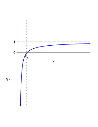
On the contrary, if the condition (17) is not met, then will not display extreme values. Due to the asymptotic behavior of (which states that for small positive values of , will be increasing, and that it will approach one asymptotically as ), will represent the gravitational potential of a black hole with a single horizon as seen in Fig. 3 Top.
A.4 Case
In a similar way, the condition (17) is not necessarily met when . When the choice of the allows the condition (17) to be met, then displays a minimum at and a maximum corresponds to a maximum. That is, for these values of , both extrema are on the interval of no physical significance. However, we can still obtain important information from the asymptotic behaviour of . As mentioned above, the signs of and will imply that the function , in the interval will start increasing from and approach one asymptotically from below, representing a black hole with a single horizon (see Fig. 3 Top).
A.5 Case
Let us now consider the scenario in which all the are negative, which means that the condition (17) may or may not be met. As such, it is important to make a separate analysis, as in the previous cases. If the condition, is met we notice that corresponds to a minimum and corresponds to a maximum. Moreover, we notice that for these values of , both extrema will always be on the interval with the minimum followed by the maximum. A quick analysis of the asymptotic behavior shows that, even though we have more extrema than in previous cases, the maximum number of horizons will be two. The reason for this is that, while the function starts decreasing in , then showcases a minimum and then a maximum, there is not additional crossing of the horizontal axis (since will approach one from above as approaches infinity). For clarity, see Fig. 2 Bottom.
Additionally, we can determine when this solution will display two, one or no horizons through the inequality (18). If the strict inequality is met, will represent the gravitational potential of a black hole with two horizons (Fig. 2 Bottom black curve), while the case in which the equality is met strictly would correspond to the extremal case (Fig. 2 Bottom red curve). On the contrary, if the condition (18) is not met, a horizon will not be formed and will not be associated to a black hole configuration.
Lastly, if the condition (17) is not met, then, will not display extreme values. Due to the previously mentioned asymptotic behavior of , there will be no such that . As a result, this case will not correspond to a black hole solution either.
A.6 Case (no solutions)
Finally, if the condition (17) is met and , the analysis of expressions (15)-(16) yields to being a minimum and corresponding to a maximum. However, this same set of equations shows that both extrema will be on the interval of no physical significance (that is, will not display extreme values in the interval ). Furthermore, the asymptotic behavior of shows that, for small positive values of , decreases from infinity and eventually approaches one from above as approaches infinity. This asymptotic behavior implies that, unless there are maxima and minima in between these regions of , the function will not cross the horizontal axis in . Since we have established that all the extreme values are in the region , there is no such that (all intersections will occur at ). As a result, this case will not showcase any horizons and thus, does not correspond to a black hole solution.
References
- [1] J. M. Maldacena, Int. J. Theor. Phys. 38, 1113-1133 (1999) doi:10.1023/A:1026654312961 [arXiv:hep-th/9711200 [hep-th]].
- [2] R. G. Cai, Y. Liu and Y. W. Sun, JHEP 10, 080 (2009) doi:10.1088/1126-6708/2009/10/080 [arXiv:0909.2807 [hep-th]].
- [3] E. Ayon-Beato, A. Garbarz, G. Giribet and M. Hassaine, Phys. Rev. D 80 (2009), 104029 doi:10.1103/PhysRevD.80.104029 [arXiv:0909.1347 [hep-th]].
- [4] E. Ayon-Beato, A. Garbarz, G. Giribet and M. Hassaine, JHEP 04, 030 (2010) doi:10.1007/JHEP04(2010)030 [arXiv:1001.2361 [hep-th]].
- [5] M. Alishahiha and R. Fareghbal, Phys. Rev. D 83, 084052 (2011) doi:10.1103/PhysRevD.83.084052 [arXiv:1101.5891 [hep-th]].
- [6] V. Pravda, A. Pravdova, J. Podolsky and R. Svarc, [arXiv:2012.08551 [gr-qc]].
- [7] R. Svarc, J. Podolsky, V. Pravda and A. Pravdova, Phys. Rev. Lett. 121, no.23, 231104 (2018) doi:10.1103/PhysRevLett.121.231104 [arXiv:1806.09516 [gr-qc]].
- [8] E. A. Bergshoeff, O. Hohm and P. K. Townsend, Phys. Rev. Lett. 102, 201301 (2009) doi:10.1103/PhysRevLett.102.201301 [arXiv:0901.1766 [hep-th]].
- [9] E. A. Bergshoeff, O. Hohm and P. K. Townsend, Phys. Rev. D 79, 124042 (2009) doi:10.1103/PhysRevD.79.124042 [arXiv:0905.1259 [hep-th]].
- [10] J. Oliva, D. Tempo and R. Troncoso, JHEP 07, 011 (2009) doi:10.1088/1126-6708/2009/07/011 [arXiv:0905.1545 [hep-th]].
- [11] H. Lu and C. N. Pope, Phys. Rev. Lett. 106 (2011), 181302 doi:10.1103/PhysRevLett.106.181302 [arXiv:1101.1971 [hep-th]].
- [12] G. Anastasiou, R. Olea and D. Rivera-Betancour, Phys. Lett. B 788 (2019), 302-307 doi:10.1016/j.physletb.2018.11.021 [arXiv:1707.00341 [hep-th]].
- [13] G. Anastasiou, I. J. Araya, C. Corral and R. Olea, JHEP 2021 (2021) no.7, 156 doi:10.1007/JHEP07(2021)156 [arXiv:2105.02924 [hep-th]].
- [14] J. Plebánski, Lectures on Non-Linear Electrodynamics (Nordita, 1968).
- [15] Mie, Gustav, Ann. Phys. Lpz 37 (1912), 511-534 doi:https://doi.org/10.1002/andp.19123420306
- [16] Born M., Proc. R. Soc. Lond. A, 143, 410-437, (1934) doi: https://doi.org/10.1098/rspa.1934.0010
- [17] Born M. and Infeld L., Proc. R. Soc. Lond. A 144, 425-451, (1934). https://doi.org/10.1098/rspa.1934.0059
- [18] Born M. and Infeld L., Proc. R. Soc. Lond. A 150, 141-166 (1935). https://doi.org/10.1098/rspa.1935.0093
- [19] P. Weiss, Proc. Cambridge Phil. Soc. 33 (1937) no.1, 79-93 doi:10.1017/S0305004100016807
- [20] Infeld L. Proc. Cambridge Phil. Soc., vol. 32, 1936, p. 127-137. doi:10.1017/S0305004100018922
- [21] Infeld L. (1937) Proc. Cambridge Phil. Soc., vol. 33, 1937, p. 70-78. doi:10.1017/S0305004100016790
- [22] Humberto Salazar I., Alberto García, and Jerzy Plebański, Journal of Mathematical Physics28, 2171 (1987); doi: 10.1063/1.527430
- [23] E. Ayon-Beato and A. Garcia, Phys. Rev. Lett. 80 (1998), 5056-5059 doi:10.1103/PhysRevLett.80.5056 [arXiv:gr-qc/9911046 [gr-qc]].
- [24] E. Ayon-Beato and A. Garcia, Gen. Rel. Grav. 31 (1999), 629-633 doi:10.1023/A:1026640911319 [arXiv:gr-qc/9911084 [gr-qc]].
- [25] E. Ayon-Beato and A. Garcia, Phys. Lett. B 464 (1999), 25 doi:10.1016/S0370-2693(99)01038-2 [arXiv:hep-th/9911174 [hep-th]].
- [26] E. Ayon-Beato and A. Garcia, Phys. Lett. B 493 (2000), 149-152 doi:10.1016/S0370-2693(00)01125-4 [arXiv:gr-qc/0009077 [gr-qc]].
- [27] E. Ayon-Beato and A. Garcia, Gen. Rel. Grav. 37 (2005), 635 doi:10.1007/s10714-005-0050-y [arXiv:hep-th/0403229 [hep-th]].
- [28] A. Alvarez, E. Ayón-Beato, H. A. González and M. Hassaïne, JHEP 06 (2014), 041 doi:10.1007/JHEP06(2014)041 [arXiv:1403.5985 [gr-qc]].
- [29] A. A. Garcia-Diaz, [arXiv:2112.06302 [gr-qc]].
- [30] A. A. G. Díaz, [arXiv:2201.10682 [gr-qc]].
- [31] E. Ayón-Beato, [arXiv:2203.12809 [gr-qc]].
- [32] M. Hassaine and C. Martinez, Phys. Rev. D 75 (2007), 027502 doi:10.1103/PhysRevD.75.027502 [arXiv:hep-th/0701058 [hep-th]].
- [33] M. Hassaine and C. Martinez, Class. Quant. Grav. 25 (2008), 195023 doi:10.1088/0264-9381/25/19/195023 [arXiv:0803.2946 [hep-th]].
- [34] H. Maeda, M. Hassaine and C. Martinez, Phys. Rev. D 79 (2009), 044012 doi:10.1103/PhysRevD.79.044012 [arXiv:0812.2038 [gr-qc]].
- [35] S. Habib Mazharimousavi, M. Halilsoy and O. Gurtug, Eur. Phys. J. C 74 (2014) no.1, 2735 doi:10.1140/epjc/s10052-014-2735-4 [arXiv:1304.5206 [gr-qc]].
- [36] J. Diaz-Alonso and D. Rubiera-Garcia, J. Phys. Conf. Ser. 314 (2011), 012065 doi:10.1088/1742-6596/314/1/012065 [arXiv:1301.3648 [gr-qc]].
- [37] D. Roychowdhury, Phys. Lett. B 718 (2013), 1089-1094 doi:10.1016/j.physletb.2012.11.019 [arXiv:1211.1612 [hep-th]].
- [38] J. Jing, Q. Pan and S. Chen, JHEP 11 (2011), 045 doi:10.1007/JHEP11(2011)045 [arXiv:1106.5181 [hep-th]].
- [39] H. A. Gonzalez, M. Hassaine and C. Martinez, Phys. Rev. D 80 (2009), 104008 doi:10.1103/PhysRevD.80.104008 [arXiv:0909.1365 [hep-th]].
- [40] M. H. Dehghani, C. Shakuri and M. H. Vahidinia, Phys. Rev. D 87 (2013) no.8, 084013 doi:10.1103/PhysRevD.87.084013 [arXiv:1306.4501 [hep-th]].
- [41] A. Bokulić, T. Jurić and I. Smolić, Phys. Rev. D 103 (2021) no.12, 124059 doi:10.1103/PhysRevD.103.124059 [arXiv:2102.06213 [gr-qc]].
- [42] H. S. Liu and H. Lü, JHEP 12 (2014), 071 doi:10.1007/JHEP12(2014)071 [arXiv:1410.6181 [hep-th]].
- [43] M. Bravo-Gaete and M. M. Juárez-Aubry, Class. Quant. Grav. 37 (2020) no.7, 075016 doi:10.1088/1361-6382/ab7694 [arXiv:2002.10520 [hep-th]].
- [44] M. Bravo-Gaete and M. Hassaine, Phys. Rev. D 91 (2015) no.6, 064038 doi:10.1103/PhysRevD.91.064038 [arXiv:1501.03348 [hep-th]].
- [45] R. M. Wald, Phys. Rev. D 48, no. 8, R3427 (1993) doi:10.1103/PhysRevD.48.R3427 [gr-qc/9307038].
- [46] V. Iyer and R. M. Wald, Phys. Rev. D 50, 846 (1994) doi:10.1103/PhysRevD.50.846 [gr-qc/9403028].
- [47] W. Kim, S. Kulkarni and S. H. Yi, Phys. Rev. Lett. 111, no. 8, 081101 (2013) [arXiv:1306.2138 [hep-th]].
- [48] Y. Gim, W. Kim and S. H. Yi, JHEP 1407, 002 (2014) [arXiv:1403.4704 [hep-th]].
- [49] L. F. Abbott and S. Deser, Nucl. Phys. B 195, 76 (1982). doi:10.1016/0550-3213(82)90049-9
- [50] S. Deser and B. Tekin, Phys. Rev. Lett. 89, 101101 (2002) doi:10.1103/PhysRevLett.89.101101 [hep-th/0205318].
- [51] S. Deser and B. Tekin, Phys. Rev. D 67, 084009 (2003) doi:10.1103/PhysRevD.67.084009 [hep-th/0212292].
- [52] L. Smarr, Phys. Rev. Lett. 30 (1973), 71-73 [erratum: Phys. Rev. Lett. 30 (1973), 521-521] doi:10.1103/PhysRevLett.30.71
- [53] M. Bravo-Gaete, S. Gomez and M. Hassaine, Phys. Rev. D 92 (2015) no.12, 124002 doi:10.1103/PhysRevD.92.124002 [arXiv:1510.04084 [hep-th]].
- [54] M. Bravo-Gaete, C. G. Gaete, L. Guajardo and S. G. Rodríguez, Phys. Rev. D 104, no.4, 044027 (2021) doi:10.1103/PhysRevD.104.044027 [arXiv:2103.15634 [gr-qc]].
- [55] H. S. Liu, H. Lu and C. N. Pope, Phys. Rev. D 92 (2015), 064014 doi:10.1103/PhysRevD.92.064014 [arXiv:1507.02294 [hep-th]].
- [56] A. Chamblin, R. Emparan, C. V. Johnson and R. C. Myers, Phys. Rev. D 60 (1999), 104026 doi:10.1103/PhysRevD.60.104026 [arXiv:hep-th/9904197 [hep-th]].
- [57] A. Edery and Y. Nakayama, JHEP 11 (2019), 169 doi:10.1007/JHEP11(2019)169 [arXiv:1908.08778 [hep-th]].
- [58] A. Álvarez, M. Bravo-Gaete , M. M. Juárez-Aubry and G. Velázquez ,work in progress.
- [59] S. Deser, H. Liu, H. Lu, C. N. Pope, T. C. Sisman and B. Tekin, Phys. Rev. D 83, 061502 (2011) doi:10.1103/PhysRevD.83.061502 [arXiv:1101.4009 [hep-th]]. [60]
- [60] M. Bravo-Gaete, M. M. Juarez-Aubry and G. Velazquez-Rodriguez, [arXiv:2112.01483 [hep-th]].
- [61] A. Karch and B. Robinson, JHEP 12 (2015), 073 doi:10.1007/JHEP12(2015)073 [arXiv:1510.02472 [hep-th]].
- [62] D. Kubiznak and R. B. Mann, Can. J. Phys. 93 (2015) no.9, 999-1002 doi:10.1139/cjp-2014-0465 [arXiv:1404.2126 [gr-qc]].
- [63] D. Kubiznak, R. B. Mann and M. Teo, Class. Quant. Grav. 34 (2017) no.6, 063001 doi:10.1088/1361-6382/aa5c69 [arXiv:1608.06147 [hep-th]].
- [64] M. Sinamuli and R. B. Mann, Phys. Rev. D 96 (2017) no.8, 086008 doi:10.1103/PhysRevD.96.086008 [arXiv:1706.04259 [hep-th]].
- [65] A. R. Brown, D. A. Roberts, L. Susskind, B. Swingle and Y. Zhao, Holographic Complexity Equals Bulk Action?, Phys. Rev. Lett. 116, no.19, 191301 (2016), [arXiv:1509.07876 [hep-th]].
- [66] A. R. Brown, D. A. Roberts, L. Susskind, B. Swingle and Y. Zhao, Complexity, action, and black holes, Phys. Rev. D 93, no.8, 086006 (2016), [arXiv:1512.04993 [hep-th]].
- [67] P. Kovtun, D. T. Son and A. O. Starinets, Holography and hydrodynamics: Diffusion on stretched horizons, JHEP 0310, 064 (2003), [hep-th/0309213].
- [68] P. Kovtun, D. T. Son and A. O. Starinets, Viscosity in strongly interacting quantum field theories from black hole physics, Phys. Rev. Lett. 94, 111601 (2005), [arXiv:hep-th/0405231 [hep-th]].
- [69] D. T. Son and A. O. Starinets, JHEP 09 (2002), 042 doi:10.1088/1126-6708/2002/09/042 [arXiv:hep-th/0205051 [hep-th]].