Also at ]Universal Biology Institute, The University of Tokyo, 7-3-1, Hongo, Bunkyo-ku, Tokyo 113-8654, Japan.
Thermodynamic and Stoichiometric Laws Ruling the Fates of Growing Systems
Abstract
We delve into growing open chemical reaction systems (CRSs) characterized by autocatalytic reactions within a variable volume, which changes in response to these reactions. Understanding the thermodynamics of such systems is crucial for comprehending biological cells and constructing protocells, as it sheds light on the physical conditions necessary for their self-replication. Building on our recent work, where we developed a thermodynamic theory for growing CRSs featuring basic autocatalytic motifs with regular stoichiometric matrices, we now expand this theory to include scenarios where the stoichiometric matrix has a nontrivial left kernel space. This extension introduces conservation laws, which limit the variations in chemical species due to reactions, thereby confining the system’s possible states to those compatible with its initial conditions. By considering both thermodynamic and stoichiometric constraints, we clarify the environmental and initial conditions that dictate the CRSs’ fate—whether they grow, shrink, or reach equilibrium. We also find that the conserved quantities significantly influence the equilibrium state achieved by a growing CRS. These results are derived independently of specific thermodynamic potentials or reaction kinetics, therefore underscoring the fundamental impact of conservation laws on the growth of the system.
I Introduction
Chemical thermodynamics provides solid physical principles for explaining the energetics and for predicting the fate of chemical reaction processes [1, 2]. Applications of these principles to autocatalytic reactions are essential to elucidate physical constraints on the capability of self-replication [3, 4]. In the self-replication process, both the chemical components and the encapsulating volume of the system have to grow in a coherent manner [5, 6, 7, 8]. This consideration introduces a unique theoretical challenge to establish the thermodynamic consistency between autocatalytic reactions and volume expansion because the conventional chemical thermodynamics is based solely on the density (concentration) of chemicals, presuming a constant volume [9, 10, 11, 12, 13, 14, 15, 16, 17, 18].
We have recently established a thermodynamic theory for growing systems, in which the number of chemicals and the volume are treated based on the rigorous thermodynamic basis [19]. Accordingly, the theory generally formulates physical conditions to realize the growth of the system, identifies several thermodynamic constraints for the possible states of the growing system, and derives the form of entropy production and heat dissipation accompanying growth. However, this theory can only address systems with regular (full-rank) stoichiometric matrices, thus limiting its applicability to a set of minimum autocatalytic motifs [20]. Given that chemical reaction systems (CRSs) are subject to stoichiometric constraints in general, and various biological functions are robustly realized by specific stoichiometric properties [21, 22], it becomes imperative to delve into the influence of stoichiometry to growing systems for comprehensive understanding of the thermodynamics of self-replication.
In this work, we clarify how stoichiometric conservation laws shape the fate of growing systems. The stoichiometry gives rise to linear combinations of the numbers of chemicals being conserved during the dynamics of chemical reactions [9, 23, 24, 25, 12, 26, 27, 13, 14, 16, 15, 28, 29, 30]. These conservation laws stringently restrict possible changes in the number of chemicals within the stoichiometric compatibility class, defined by the stoichiometric matrix’s left kernel and the initial condition. In biological contexts, particularly in metabolic networks, these laws are crucial in linking the dynamic variations of different chemicals (metabolites) and also in providing insights into cells’ production capabilities [31, 32, 33, 34, 35, 36, 37, 38].
This study elucidates the complex interplay between thermodynamics and stoichiometric conservation laws for the growing system and its consequence to the fate of the growing systems. By disentangling the geometric relationship among chemical numbers, densities, and potentials, we establish the conditions for the system to grow, shrink, or equilibrate, while simultaneously satisfying the second law of thermodynamics and the conservation laws. Furthermore, we show that the existence of conservation laws qualitatively alter the fate of the system and the geometric properties of the equilibrium state.
These results are derived solely based on thermodynamic and stoichiometric requirements and thus remain independent of specific thermodynamic potentials or reaction kinetics. This renders our theory universally applicable, enhancing our understanding of the origins of life and the construction of protocells[39, 40, 41, 42, 43, 44, 45, 46, 47, 48, 49, 50, 51, 52, 53, 54, 55, 56, 57, 58, 59, 20, 60, 61, 62], and enabling the search for the universal laws of biological cells [63, 64, 65, 66, 67, 68, 69, 70, 71, 72, 73, 74, 75, 76].
This paper is organized as follows. We devote Sec. II to outline our main results accompanying with an illustrative example of a growing CRS. Here, we clarify the environmental and initial conditions that determine the fate of the system: growth, shrinking or equilibration. In Sec. III, we explain the geometric structure of the growing system to characterize the equilibrium state as a maximum of the total entropy function, which the system may achieve. In Sec. IV, the form of the total entropy function is further investigated to determine if the system grows or shrinks by following the second law of thermodynamics. In Sec. V, we provide a mathematical proof of our main results outlined in Sec. II. Finally, we summarize our work with further discussions in Sec. VI. For better readability, we list the symbols and notations in Appendix L.
II Outline of the main results
We outline our main results before presenting their derivations. In Sec. II.1, we give a thermodynamic setup of a growing chemical reaction system (CRS). By introducing the chemical potential space, we analyze candidates of chemical equilibrium states in Sec. II.2. By computing accessible regions of the system, we characterize the equilibrium state as an intersection of the accessible region and the candidates in Sec. II.3. In Sec. II.4, we present our main claims with the above preparation. We comment our claims for a special class of the growing CRS in Sec. II.5. These results are summarized in Table 1. Then, we demonstrate the claims by numerical simulations using a simple example of the growing CRS in Sec. II.6. Finally, in Sec. II.7, we outline the derivations of our results, which will be presented in the subsequent sections.
II.1 Thermodynamic setup
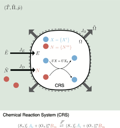
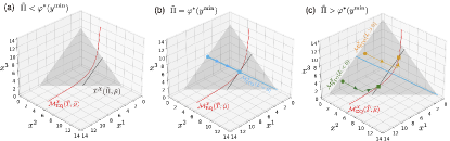
We consider the following thermodynamic setup in the present paper (Fig. 1). A growing open chemical reaction system is surrounded by an environment. We assume that the system is always in a well-mixed state (a local equilibrium state), and therefore, we can completely describe it by extensive variables . Here, and represent the internal energy and the volume of the system. denotes the number of chemicals that can move across the membrane between the system and the environment, which we call open chemicals hereafter. is the number of chemicals confined within the system; the indices and respectively run from to and from to , where and are the number of species of the open and the confined chemicals. The environment is characterized by intensive variables , where and are the temperature and the pressure; is the chemical potential corresponding to the open chemicals. Also, denote the corresponding extensive variables.
In thermodynamics, the entropy function is defined on as a concave and smooth function . We also write the entropy function for the environment as , and the total entropy can be expressed as
| (1) |
where we use the additivity of the entropy. Further, the entropy function for the system has the homogeneity. Therefore, without loss of generality, we can write it as
| (2) |
where is the entropy density and . In this work, we consider only a situation without phase transition, and therefore, we assume that is strictly concave.
The dynamics of the number of confined chemicals is described by
| (3) |
where represents the chemical reaction flux; denotes the stoichiometric matrix for the confined chemicals (see Fig. 1). The index runs from to , where is the number of reactions. Also, Einstein’s summation convention has been employed in Eq. (3) for notational simplicity. By integrating Eq. (3), we obtain
| (4) |
where denotes the initial condition and is the integration of , i.e., the extent of reaction.
In this work, we assume that the stoichiometric matrix does not have the right kernel space,
| (5) |
By contrast, the left kernel space exists and generates a set of conserved quantities:
| (6) |
i.e., the vector . Here, is a basis matrix: whose row vectors form the basis of , i.e., , and runs from to . Since we are mainly interested in the growth of the system, the time evolution of should perpetually increase the number of all confined chemicals while satisfying the conservation laws (Eq. (6)). In order to realize this situation, the stoichiometric matrix should satisfy
| (7) |
which is known as the condition for the productive [20]. The productive excludes the mass conservation-type laws, the existence of which trivially precludes the number of confined chemicals to increase continuously.
The number of open chemicals changes through the reactions and the diffusions. By defining the stoichiometric matrix for open chemicals as and the diffusion fluxes as , we have
| (8) |
Example 1: To give an illustrative example, we consider the following chemical reactions:
| (9) |
Here, three confined chemicals and two open chemicals are involved in two reactions and 111One may feel that the order of the reactions in Eq. (9) is high. The reason why we consider this example is just because it is straightforward to visualize our geometric representation in Sec. III. Since and we can visualize up to three dimensional space (), relevant cases are when is one, two or three. The present example corresponds to the case in which is two. In Sec. I and II of the Supplementary material, we also consider other examples with which is one and three, respectively.. The stoichiometric matrices and for the confined and open chemicals, respectively, are
| (10) |
Since in this case, we can represent the number of confined chemicals by introducing as
| (11) |
For this example, is one, and satisfies . Thus, the reactions have the conserved quantity . We can intuitively see the conserved quantity from the chemical equations in Eq. (9) as follows. The numbers of and , i.e., and , change in the same manner: each chemical is consumed by one molecule in the forward reaction of and is produced by one in that of . Thus, the difference between and is conserved when each of the reactions occurs.
In this paper, we assume that the time scale of the chemical reactions is much slower than that of the others, i.e., . This means that we consider the isothermal and isobaric process with a balance of chemical potentials for open chemicals. This assumption allows us to separately analyze the slow dynamics of chemical reactions from the fast dynamics of the energy, the volume, and the chemical diffusion. As shown in Appendix A, our dynamics is effectively governed by Eq. (3), and the other variables are rapidly relaxed to the values at the equilibrium state of the fast dynamics. As a result, is obtained as a function of .
With the above assumptions, we obtain the following expression for the total entropy (see Eq. (74) in Appendix A),
| (12) |
where . Here, is the partial grand potential density, which is given by a Legendre transformation of :
| (13) |
Note that is strictly convex because is strictly concave. The volume is variationally determined under isobaric conditions as
| (14) |
Example 2: If we assume that the system and the environment are composed of ideal gas or solution, the partial grand potential density is expressed as
| (15) |
where is the gas constant, and and are the standard chemical potentials of the confined and the open chemicals, respectively[78].
Since we assume that the environment also consists of the ideal gas, the chemical potential in Eq. (15) is represented as
| (16) |
where is the density of the open chemicals in the environment. Furthermore, Eq. (14) gives the following expression for the volume ,
| (17) |
which corresponds to the equation of state.
From Eq. (14), the density is obtained by a nonlinear function of as
| (18) |
Since is homogeneous, we have for . This fact implies that induces one-to-one correspondence between rays in the number space and points in the density space . Here, we write the corresponding ray to a density , i.e., the fiber of for , as
| (19) |
II.2 Candidates of chemical equilibrium states
We define the full grand potential density by the Legendre transformation of in Eq. (13):
| (20) |
We mention that is strictly convex. Because of the one-to-one correspondence of the Legendre transformation by and , a state of the system is equivalently specified either by the density of the confined chemicals or by its Legendre dual variable 222The inverse transformation is given by . The existence of one-to-one correspondence between and is physically reasonable (See Sec. III.1).. The thermodynamic interpretation of is the corresponding chemical potential to . In addition, can be interpreted as the pressure of the system at the state . Recalling the one-to-one correspondence by between rays in and points in , we notice that there exists the one-to-one correspondence between rays in and points in . Here, we write the corresponding ray to a chemical potential as
| (21) |
The chemical equilibrium states are given by the balance of chemical potentials between reactants and products [78]:
| (22) |
Thus, we can obtain the candidates of chemical equilibrium states by the solutions to Eq. (22):
| (23) |
which we term the equilibrium manifold. Here, we note that , because we have assumed in Eq. (5), i.e., .
II.3 An equilibrium state as the intersection
The reaction dynamics in Eq. (3) with its conserved quantities restricts the accessible region in as
| (24) |
This subspace is known as the stoichiometric compatibility class[80]. By using the mappings in Eq. (18) and , the accessible regions in the density space and the chemical potential space are respectively obtained as
| (25) | ||||
| (26) |
Since the system evolves only on , the equilibrium state to which the system converges is represented by the intersection:
| (27) |
if it is not empty. If the intersection is empty, the system never converges to the equilibrium state and the growth of the volume may happen.
II.4 Main claims of the present paper
In this subsection, we state our two main claims of this work before presenting their derivations in the following sections.
Our first claim provides the conditions to determine the fate of the system, i.e., growth, shrinking or equilibration. To formulate our claim, we define as
| (28) |
Note that the productivity of in Eq. (7) guarantees the existence and the uniqueness of (see the latter half of Appendix F). This gives the chemical equilibrium state whose pressure is the minimum in the candidates, .
Claim 1
The fate of the system is classified by and the conserved quantities in Eq. (6) as follows (see also Table 1):
-
1.
If , the system grows and finally diverges for any .
-
2.
If , the system converges to an equilibrium state when , whereas it grows when .
-
3.
If , the system shrinks and finally vanishes when , whereas it converges to an equilibrium state when .
Here, represents the case in which for all the components of in Eq. (6), and indicates that at least one of the components is not zero.
We first notice that one of the conditions in the claim is given by the sign of . Here, represents the minimum pressure of the system within (see Eq. (28)), whereas is the pressure of the environment. The growth of the system occurs independently of the value of when , because the environmental pressure can not prevent the system from growing by counteracting any internal pressures for .
The equilibration becomes possible only when is fulfilled. For the singular case of , the equilibration occurs only when the minimum internal pressure perfectly balances with the external one, namely, . When , the system shrinks and approaches as because the external pressure dominates the internal one at the equilibrium state. For the generic , the fate of the system is qualitatively altered. The system equilibrates even if owing to the non-singular conservation laws, which prevent from approaching , i.e., shrinking. In fact, the equilibrium state can have a higher pressure in this case than , and it balances with the external pressure . In addition, the system grows for .
From claim 1, the system converges to an equilibrium state when (1) and , and (2) and . For these cases, our second claim describes how the equilibrium states appear in the number space .
Claim 2
In the number space , the equilibrium states appear as follows (see also Table 1):
-
1.
When and , the equilibrium state to which the system converges depends on the initial condition and the functional form of the reaction flux . Such an equilibrium state lies on the ray in Eq. (21).
-
2.
When and , the equilibrium state is uniquely determined, irrespective of the initial condition and the form of the reaction flux .
| Regular | |||
|---|---|---|---|
| Growing | Growing | Growing | |
| Growing | EQ (D) | EQ (D) | |
| EQ (I) | Shrinking | Shrinking |
II.5 Regular stoichiometric matrix
The fates of the system for the singular case of are basically the same as the case that is regular; no conservation laws exist so that , and from Eq. (5) 333Note that regular is productive in Eq. (7). (see Sec. V.3 for the reason why regular can be interpreted as ). Thus, the two claims clarify that the existence of conservation laws is a fundamental determinant of the fate of the growing system. We investigated the case of regular in our previous work [19] (see also 444In Sec. II of the Supplementary material, we show an example when is regular in which the dimension of is zero and that of is three.). For comparison, we summarize the results here (see the cases for and regular in Table 1).
For a regular , the candidates of chemical equilibrium states, in Eq. (23), consist of precisely one point . Here, we note that is identical with by Eq. (28). Then, we obtain
Corollary 1
When the stoichiometric matrix is regular, the fate of the system is classified by as follows (see also Table 1):
-
1.
If , the system grows and finally diverges.
-
2.
If , equilibrium states form the ray in Eq. (21). The system converges to one of them, depending on the initial condition and the functional form of the reaction flux .
-
3.
If , the system shrinks and finally vanishes.
This statement corresponds to claim 1 in [19].
II.6 Numerical demonstrations
In this subsection, we demonstrate our claims by using the specific reactions in Example 1 with the ideal gas case (see Example 2).
We first calculate the equilibrium manifold in Eq. (23) to obtain in Eq. (28). For the specific reactions in Eq. (9) and the stoichiometric matrices in Eq. (10), the simultaneous equations in Eq. (22) are written as
| (29) |
The solutions are expressed as
| (30) |
where is the coordinate of . The set of solutions in Eq. (30) represents the equilibrium manifold .
Second, using Eqs (15) and (20), the full grand potential density is obtained for the ideal gas or solution as
| (31) |
Using the solutions in Eq. (30), is represented on as
| (32) |
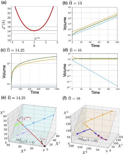
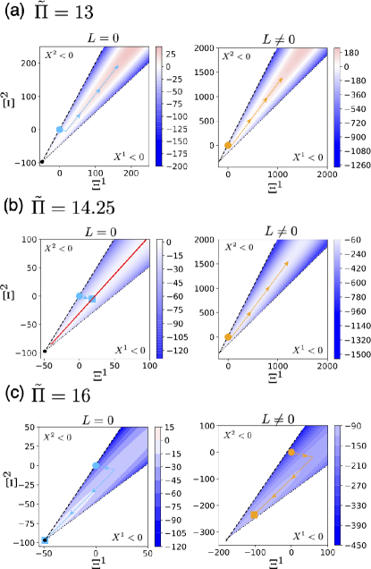
In Fig. 2(a), we numerically plot the pressure on . Here, we have a unique that attains the minimum . Substituting it into Eq. (30), we obtain and the minimum pressure . With the parameters given in the caption, .
To demonstrate that the fate of the system is classified by and the conserved quantities in claim 1, we show numerical simulations of the dynamics, Eq. (3). From the solution , the volume of the system is determined by the equation of state, Eq. (17). To numerically solve Eq. (3) with the stoichiometric matrix in Eq. (10), we employ the mass-action kinetics with the local detailed balance condition to specify the flux function (see Appendix B).
Claim 1: In Fig. 2(b-d), we show numerical trajectories of the volume from three initial conditions for different pressures . The color of curves corresponds to each initial condition. The fate of the system changes with as follows. When (Fig. 2(b)), the volume of the system increases with time from any initial conditions. As increases to (Fig. 2(c)), the trajectory from an initial condition with in light blue achieves an equilibrium state, whereas trajectories from the other two with continue growing. As increases further, (Fig. 2(d)), the trajectory with in light blue decreases and the system shrinks. By contrast, those from the other two with achieve equilibrium states. These numerical results demonstrate the claim 1.
Claim 2: In Fig. 2(e,f), we demonstrate the time evolution of the number . When and , the equilibrium state to which the system converges depends on the initial conditions in . Furthermore, it indeed lies on the ray , which is given by Eq. (21) (see Fig. 2(e)). In our numerical simulation, we compute it as follows. From , we obtain the corresponding density by using Eq. (31). The ray is plotted by the one which includes . When and , the system indeed converges to the unique equilibrium state, irrespective of the initial conditions in (see Fig. 2(f)).
II.7 Outline of the derivations of claims 1 and 2, and Corollary 1
The fates of the system stated in claims 1 and 2, and Corollary 1 are summarized in Table 1. Before closing this section, we outline their derivations, which will be presented in the subsequent sections. They will be derived in two steps. In the first step, we investigate the existence of an equilibrium state, that is the intersection in Eq. (27). In Sec. III, we will show that the intersection is not empty in the case for and in the case for of claim 1, and is empty for the other cases. This will be summarized in Theorem 1. Following Theorem 1, we derive claim 2 from the correspondence in Eq. (21) between the number space and the chemical potential space . In the second step, when the intersection is empty, we investigate the landscape of the total entropy function to classify whether the system grows or shrinks in Sec. IV. We will show that the system has two possibilities for : it grows when is not bounded above, or it shrinks when the supremum of is at the origin . By contrast, the system always grows for when the intersection is empty because is not bounded above. This will be summarized in Theorem 2. Mathematical proofs of Theorems 1 and 2, and Corollary 1 will be presented in Sec. V.
III Geometric representation of equilibrium states
For the derivation of claims 1 and 2, we analyze the accessible regions in the number space , the density space and the chemical potential space by using a geometric technique. In Sec. III.1, we give the assumptions to the full grand potential density for the following mathematical treatment. In Sec. III.2, we show that the accessible region is restricted by the isobaric condition, which we term the isobaric manifold. This manifold is further partitioned by the conservation laws in Sec. III.3. After defining the equilibrium manifold as the candidates of chemical equilibrium states in Sec. III.4, we characterize the equilibrium state to which the system converges as an intersecting point of the accessible region and the equilibrium manifold in Sec. III.5. Furthermore, by using numerical simulations, we identify the conditions for the existence of the intersecting point, which we state as Theorem 1.
III.1 Assumptions to
The thermodynamic property of the system is encoded in the full grand potential density (see Eq. (20)). Here, is the chemical potential of the confined chemicals, and represents the pressure of the system at the state . In this work, we assume that is a smooth and strictly convex function on , and the image of the associated Legendre transformation,
| (33) |
is equal to . In addition, we assume the following properties; (1) strictly increases with for an arbitrary fixed . (2) when . They are satisfied in most thermodynamic systems such as the ideal gas in Eq. (31).
Furthermore, we assume that the mapping is bijective, and we consider that its inverse map is given by (see Eq. (13) for ). By using this, the above property (2) is rephrased as when .
Finally, we assume that the pressure of the environment is greater than , to guarantee that the volume is uniquely determined (see Appendix C). Here, denotes the minimum pressure that the system can take as
| (34) |
The second equality holds from the above property (1).
III.2 The isobaric manifold and the projection
We remind that the density is given by the mapping in Eq. (18):
| (35) |
The range of the mapping describes possible states of the density under the isobaric condition. To calculate the range, we compute the volume by solving the minimization in Eq. (14). Its critical equation is given by
| (36) |
Therefore, the possible region in under the isobaric condition is constrained in
| (37) |
which we call the isobaric manifold. Since the range of is represented in Eq. (37), we find that the mapping is a projection of into along the ray which includes .
Example 3: For the ideal gas case, by substituting in Eq. (15) into Eq. (37), we obtain
| (38) |
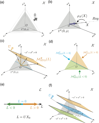
where is the density of the open chemicals in the environment (see Eq. (16)). Thus, the isobaric manifold in represents a simplex for the ideal gas case (Fig. 3(a)).
The mapping is the projection of into this simplex (see Fig. 3(b)).
Finally, by using the mapping , the isobaric manifold in is represented as
| (39) |
which is straightforward to interpret that the pressure of the system at the chemical potential is balanced with in this manifold.
III.3 The stoichiometric manifold as partition of the isobaric manifold
The accessible subspace of the state from an initial condition in Eq. (4) is
| (40) |
which we call the stoichiometric manifold in .
By applying the mapping to , we have the stoichiometric manifold in the density space as
| (41) |
where is arbitrary. Using the mapping , the stoichiometric manifold in the chemical potential space is given by
| (42) |
Example 4: For the specific stoichiometric matrix in Eq. (10), is schematically depicted in Fig. 3(c,d) by applying the mapping to .
For further investigations, we define the following manifold in as
| (43) |
and that in as
| (44) |
These manifolds correspond to the stoichiometric manifolds with conserved quantities under the isochoric condition [78]. Hereafter, we term the isochoric stoichiometric manifolds.
Using these manifolds, the stoichiometric manifold under isobaric condition is represented as follows:
| (45) |
and
| (46) |
For arbitrary , we find and, correspondingly, . Hence, each ray in the space of conserved quantities characterizes these manifolds (see also Example 5 below and Fig. 3(d-f)). To be more precise, for any , holds. We denote the stoichiometric manifold corresponding to a ray as .
When , the stoichiometric manifold in is written as
| (47) |
Since the dimension of in Eq. (45) vanishes for , we obtain . In addition, for any given , we find that when . Thus, the stoichiometric manifold forms an interface of all the stoichiometric manifolds . These properties hold similarly in by replacing the superscript with .
The above statements are summarized as follows.
Lemma 1
Let denote a ray in the space of conserved quantities. For every , the corresponding stoichiometric manifold exists and the set of the stoichiometric manifolds partitions the isobaric manifold . In addition, their interface is given by the stoichiometric manifold . The isobaric manifold in the chemical potential space is similarly partitioned by stoichiometric manifolds (replace the superscript with ).
Example 5: In Fig. 3(d-f), we schematically depict the partition of the isobaric manifold by the stoichiometric manifolds for the ideal gas case.
III.4 The equilibrium manifold
In this subsection, we confirm that the candidates of the equilibrium states are given by Eq. (23).
The equilibrium states of the chemical reaction dynamics are given by the maxima of the total entropy with respect to the extent of reaction . From the differentiation of Eq. (12) and using Eq. (14), we have the critical equation as
| (48) |
Thus, at any equilibrium states, the density satisfies
| (49) |
By using the correspondence , it is represented as
| (50) |
which confirms the balance of chemical potentials between reactants and products at the chemical equilibrium (see Eq. (22)).
The set of solutions to Eq. (49) represents the candidates of the equilibrium states in the density space , which we call an equilibrium manifold:
| (51) |
and in the chemical potential space as
| (52) |
We note that the equilibrium manifold is an affine subspace in , whereas it is generally curved in . In addition, using the basis matrix of and solving Eq. (50), the manifold in Eq. (52) is rewritten as
| (53) |
where is a particular solution to Eq. (50) and represents a coordinate of .
III.5 The equilibrium state as an intersection
If the intersection is not empty, the system converges to the equilibrium state. We can compute the equilibrium state in by using Eqs. (42) and (52). Similarly, we obtain the corresponding state in as by using Eq. (41) and (51). In this subsection, we numerically confirm the convergence in by the dynamics in Eq. (3) using the specific setup in Sec. II.6.
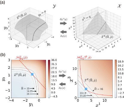
We first consider the equilibrium manifold. The points in are written in Eq. (30). Here, the second component is constant . Thus, is a one-dimensional line located on the plane in (see the left panel of Fig. 4 (a) for the plane , and the red line in the left panel of Fig. 4 (b) for ). By applying the mapping , we can compute . For the ideal gas case in Eq. (31), the mapping is represented as . Thus, the points in are computed as
| (54) |
where plays a role of the coordinate of . We note that the second component is also constant . Thus, is a one-dimensional curve located on the plane . (see the red curve in the right panel of Fig. 4(b)).
We next consider whether the intersection is empty or not. As the pressure increases, the number of intersecting points change as follows. When , the intersecting point does not exist (see the right panel of Fig. 4(b)). When , the intersection appears as the unique contact point corresponding to . When , the intersection consists of two points. The above situation holds similarly in (see the left panel of Fig. 4(b)).
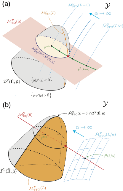
We further depict the intersection by the three dimensional plot in Fig. 5. From Fig. 3(d), is partitioned by the stoichiometric manifolds. When (Fig. 5(b)), the intersection lies on . When , the two intersecting points belong to each of for and , respectively (see Fig. 5(c)). Thus, for a given , the intersecting point is uniquely determined and it depends on a ray in the space of the conserved quantities (see Fig. 3(e) and Lemma 1).
In Fig. 5(b,c), we also show the time evolution of the system in the numerical simulation. Indeed, the system converges to the intersection .
The above numerical result is an instance of the following theorem.
Theorem 1
The system converges to the intersecting point if it exists. Its existence is classified as follows:
-
1.
.
-
2.
-
3.
where the intersecting point is uniquely determined for a given , and it depends on a ray in the space of conserved quantities.
A mathematical proof of this theorem will be shown in Sec. V.
From Theorem 1, we can derive claim 2 as follows. For the case 1 of claim 2 in which and , Theorem 1 states that the intersection consists of . From Eq. (21), this is mapped to a ray in the number space . In addition, from Eq. (40) indicates that if for arbitrary . This means that all the points on the ray is in . Thus, all the points on the ray are equilibrium states and the system converges to one of them. The state is not uniquely determined only by the entropy function and depends on the initial conditions and the functional form of . For the case 2 of claim 2 in which and , Theorem 1 states that the intersection exists as . This also corresponds to a ray in the number space . Since is an affine subspace which does not include the origin , the intersection between and an arbitrary ray is represented by a point. Thus, the equilibrium state is uniquely determined in this case.
Theorem 1 states the cases when the system converges to an equilibrium state in our claim 1. In the next section, we will investigate the case when the system does not converge to an equilibrium state, that is .
IV Form of the total entropy function
When the intersection is empty, the system cannot converge to an equilibrium state, and it is expected that the system grows or shrinks. In this section, we observe if the system grows or shrinks by numerical plots of the total entropy function.
If , the total entropy function can not have the maximum inside of (see Sec. III.4). Thus, the functional form of has the following two possibilities: (1) is not bounded above. (2) is bounded above, but the supremum exists on the boundary of . In the first case, we find for , because the second law requires that the system must climb up the unbounded landscape of the total entropy function. Since we assume , we get for . In addition, for (see Appendix E). Thus, if is not bounded above, the volume grows. In the second case, we can further show that the supremum is possible only at the origin (see Sec. V.2). Thus, the volume is shrinking and finally vanishes.
In the following part of this section, we numerically plot the landscape of the total entropy function to determine the fate of the system. In Fig. 6, we plot the total entropy function in Eq. (12) for our example setup (see Example 1 and Example 2). Following Theorem 1, the intersection is empty for the cases (1) , (2) and , and (3) and ,
In the case (1) , the total entropy function is not bounded above for both of and (see Fig. 6(a)). Indeed, in the reaction dynamics of Eq. (3). In the case (2) and , is still not bounded above and (see the right panel of Fig. 6(b)). In the case (3) and , the supremum of is at the origin of the number space . The system tends to approach the origin (see the left panel of Fig. 6(c)).
The above numerical result demonstrates the following theorem.
Theorem 2
When , the landscape of is given as follows:
-
1.
If , is not bounded above.
-
2.
If and , is not bounded above.
-
3.
If and , the supremum of is at the origin of the number space .
A mathematical proof of this theorem will be shown in Sec. V.
Before closing this section, we confirm the claim 2 in the left panel of Fig.6(b) and the right panel of Fig.6(c). In the former panel, the red ray represents the set of the maxima of , which is . We can see the system converges to a point on the ray. In the latter case, the maximum of is the unique point and the system converges to it.
V Proof of the Theorems
V.1 Proof of Theorem 1
We first provide a general proof valid for arbitrary dimensions. After concluding the proof, we schematically illustrate it for three dimensional space of in Fig. 7.
To investigate the existence of the intersection , we introduce Birth’s trajectory.
Let represent the unique intersecting point between the isochoric stoichiometric manifold in Eq. (44) and the equilibrium manifold in Eq. (52):
| (55) |
The uniqueness of is guaranteed by Birch’s theorem and the point is known as Birth’s point [83, 12, 17, 78, 84] (see Appendix F). We define Birch’s trajectory by a collection of Birch’s point along a ray in the space of conserved quantities. For given , it is defined as
| (56) |
We find that for . Furthermore, from Eq. (94) in Appendix F, we get
| (57) |
Thus, the point is located at one of the end points of Birch’s trajectory, but is not included in the trajectory.
For this Birch’s trajectory, the following lemma is satisfied.
Lemma 2
is a strictly increasing function along Birch’s trajectory from the starting point .
A proof of this lemma is shown in Appendix G.
By employing Birch’s trajectory, we can represent the intersection for as
| (58) |
where we use Eqs. (46), (55), and (56). For , the intersection is
| (59) |
From Lemma 2, we can determine the existence of the intersection by the position of the starting point . When , the starting point is located in the superlevel set: . Taking into account the fact that is the level set, the intersecting point does not exist for any . When , the starting point is on . For , the intersecting point uniquely exists as because of Eq. (59). For , Lemma 2 indicates at any point on Birch’s trajectory . Thus, from Eq. (58), the intersecting point does not exist. When , the starting point is located in the sublevel set: . For , the intersecting point does not exist. For , the intersecting point uniquely exists.
This concludes the proof of Theorem 1.
In Fig. 7, we provide schematic illustrations in three dimensional space of for the case . To demonstrate the generality of the proof, we visualize two cases with and in the panels (a) and (b), respectively. From Eq. (6), the case in (a) has two conserved quantities, whereas the case in (b) has one conserved quantity. We also have and for the two cases, respectively, because and . The dimensions for the example in Eqs (9) and (10) correspond to the case (b), whereas the case (a) corresponds to the one investigated in Sec. I of the Supplementary material.
In the former case (Fig. 7(a)), the equilibrium manifold is represented by the two dimensional plane in red, whereas the isochoric stoichiometric manifold is given by a one-dimensional curve in light blue because and . Accordingly, the black circles represent the intersecting points in Eq. (55) for with varying . The green curve indicates Birch’s trajectory in Eq. (56), and one of the end points is located at in Eq. (57). The isobaric manifold is represented by the gray surface, which is a level set for . When , is in the sublevel set . The stoichiometric manifold is given by the orange curve from Eq. (46). Thus, the intersection is represented by the red circle, which is also the intersecting point between and in Eq. (58).
In the latter case (Fig. 7(b)), is represented by the red line, whereas is given by the two dimensional surface in light blue. The intersecting point is indicated by the black circle in Eq. (55) for with a given . In this case, the Birch’s trajectory in Eq. (56) overlaps with the red line, and one of the end points is located at in Eq. (57). The stoichiometric manifold is given by the orange surface from Eq. (46)555Similar to Fig. 3(d), the isobaric manifold is partitioned by and in this case.. Thus, the intersection is represented by the red circle.
V.2 Proof of Theorem 2
If , the system never relaxes to the equilibrium state and have the following two possibilities: (1) is not bounded above, and with time. As we noted in Sec. IV, the volume grows in this setup. (2) is bounded above and the supremum exists on the boundary of .
First, we consider the case , where does not contact with the origin. In this case, is not bounded above. To prove that, we will show that the supremum of does not exist on the boundary of as follows.
The extent of reaction provides a coordinate on the stoichiometric manifold . Since , the domain of has a boundary. We denote the coordinate of a point on a boundary by . Here, at least, one component of the vector is zero. We define the index set by . Since the origin is excluded, never has all the indices. Also, the density has zero components as for .
To investigate the gradient of on the boundary, we calculate the thermodynamic force as
| (60) |
If the supremum of does not exist on the boundary, we can find a direction from the boundary to the interior of such that increases. To be more precise, by using , this statement is mathematically phrased as follows: If the supremum of does not exist on the boundary, a vector exists such that and for all the indices . In the next paragraph, we prove the above statement.
From the assumptions to in Sec. III.1, for every , when . Thus, for all . Choose a vector satisfying for . Then, we can show that, when , from Eq. (60). This indicates that the supremum of does not exist on the boundary.
Second, we consider the case . By employing rays on , we investigate whether is bounded above or not.
Since we have assumed , we can rewrite as a function of . Using a particular solution to Eq. (50), we get
| (61) |
where
| (62) |
(see Appendix H for the details of the calculation). Here, is the Bregman divergence [86, 87, 88] induced by , which is defined as
| (63) |
and . Although Eq. (61) is apparently a function of the particular solution , the value of does not depend on the choice of as shown in Appendix I. Since only the first term depends on , we consider its landscape.
The stoichiometric manifold with , , can be described by the collection of rays in because it contacts with the origin . Since a ray in the number space corresponds to a point in the chemical potential space as in Eq. (21), the value of is constant on each ray. In addition, is increasing along each ray from the origin. Therefore, by considering the sign of , we can determine if increases along each ray in . If is positive for a ray, increases along the ray. If , is constant along the ray. If is negative for a ray, decreases along the ray.
When , we can find a point such that is positive (see Appendix J). If such a point exists, we can consider a corresponding ray in to the point . Along the ray, increases and, thus, is not bounded above. When , is negative for any except , and . Thus, the maxima of forms the ray corresponding to , that is in Eq. (21). When , we can show that any gives negative (see Appendix K). Thus, decreases along any ray and the supremum is located at the origin .
Summarizing the cases for and , we obtain Theorem 2.
V.3 Proof of Corollary 1
When is regular, the accessible region covers the whole space of , that is . Thus, can be described by the collection of rays in . This situation coincides with the one for in the previous subsection. Therefore, by employing a similar proof, we can classify the fate of the system as Corollary 1 (see also [19]).
VI Summary and Discussions
In this work, we have considered chemical thermodynamics of growing CRSs with stoichiometric conservation laws in which the stoichiometric matrix has a nontrivial left kernel space. By clarifying the conditions for the fate of the system to grow, shrink, or equilibrate, we show that the existence of conservation laws qualitatively alter the fate of the system. It is emphasized again that our results are derived by general thermodynamic and stoichiometric structures without assuming any specific thermodynamic potentials or reaction kinetics; i.e., they are obtained based solely on the second law of thermodynamics and conservation laws.
Since we are mainly interested in the growth of the system, we have assumed the productivity of the stoichiometric matrix : (see Eq. (7)). This condition allows the time evolution of so as to perpetually increase the number of all confined chemicals while satisfying the conservation laws. In the following two paragraphs, we comment on the fate of the system with the other classes of the stoichiometric matrix. Here, the complement of the productive is defined as . We divide it into two cases: (1) , and (2) and 666Note the equality in of ..
In the first case, (1) , a vector exists in such that all the components of are positive. As a result, the conserved quantity implies that the total mass of the confined chemicals are conserved, and the system must converge to the equilibrium state, i.e., the growth of the system is not possible. We refer to this type of as non-productive. A numerical example for this case is shown in Sec. III of the Supplementary material.
In the second case, (2) and , a vector exists in such that all the components of are non-negative, but does not have a vector such that all the components of are positive. This means that the mass conservation law exists for a proper subset of the confined chemicals. Thus, the volume growth of the system can still be allowed with the increase of the confined chemicals that do not participate in the mass conservation law. Although such a situation may not be biologically relevant, we refer to this type of as semi-productive. A numerical example for this case is shown in Sec. IV of the Supplementary material. According to the example, it is expected that the claims 1 and 2 still hold for the semi-productive cases.
We can possibly correlate our theoretical findings with empirical observations. Our findings suggest that the fate changes with the initial conditions (conserved quantities ) even in the same environment. We especially find that, as shown in Table 1, a CRS does not vanish and is more likely to grow when it has non-zero than when it has or a regular . If we suppose a population of the CRSs with varying initial conditions, and consider their fates in a slowly changing environment, surviving CRSs can be selective depending on , where a CRS with non-zero might be advantageous. Identifying a possible mechanism to survive in a varying environment is biologically essential, and our findings may help explain the outcome.
Nevertheless, several extensions of our theory remain to be essential as future work to understand actual experimental situations of growing protocells or biological cells.
The first extension is to consider the case when the system may relax to a state that continuously produces entropy with constant volume, namely, the conventional nonequilibrium steady state (NESS) [16, 14, 15, 10, 17, 13, 12, 9]. It is possible when the matrix has a nontrivial right kernel space, i.e., the assumption in Eq. (5) is not satisfied. It is a major challenge to understand how the growth of the system can be characterized and realized in such situations, and compatible with the NESS.
The second one is to consider a different hierarchy of the timescales in which the relaxation of the variables may not be rapid compared to the timescale of chemical reactions. Although the present work assumes that the chemical reactions are slow (see the assumptions made above Eq. (12)), there may be cases in which the timescale of other processes is slow and/or comparable with that of the chemical reactions. A typical example is when we consider cell transport processes [90]. In this case, the timescale of material exchanges between the system and the environment is relevant, and the processes may also couple with chemical reactions. In addition, the osmotic gradient (pressure difference) can play a driving force to change the volume, whereas isosmotic volume changes are also commonly known and widely investigated as a relevant process by alterations in intracellular solute content [91, 92]. It is of interest to see how the conditions for the growth of the system change with relevant processes of the thermodynamic setup.
The third one is to consider explicitly the effect of the membrane molecules. Although we neglect the tension of the membrane in this paper (see Fig. 1), it could be relevant and changes with time because the membrane molecules themselves are produced and supplied by the CRSs in biological cells. It is important to investigate if and how the effect changes the results by extending our theoretical framework.
Alternatively, it would also be promising to apply our framework to fit into an experimental technique using membrane-free compartments such as droplets based on liquid-liquid phase separation [93]. Since its nature, a rigorous thermodynamic treatment would require an extended framework in which the entropy function is not strictly concave (see the assumption made below Eq. (2)).
In all the above extensions, the present work provides basic results to clarify the role of conservation laws to the growth of protocells and biological cells.
VII Acknowledgments
The authors thank Dimitri Loutchko and Shuhei A. Horiguchi for discussions. This research is supported by JSPS KAKENHI Grant Numbers 19H05799, 21K21308, and 24K00542, and by JST CREST JPMJCR2011 and JPMJCR1927. Y. S. receives financial support from the Public\Private R&D Investment Strategic Expansion PrograM (PRISM) and programs for Bridging the gap between R&D and the IDeal society (society 5.0) and Generating Economic and social value (BRIDGE) from Cabinet Office.
References
- Callen [1985] H. B. Callen, Thermodynamics and an Introduction to Thermostatistics (John wiley & sons, New York, 1985).
- Kondepudi and Prigogine [1998] D. Kondepudi and I. Prigogine, Modern thermodynamics: from heat engines to dissipative structures (John Wiley & Sons, New York, 1998).
- von Neumann and Burks [1966] J. von Neumann and A. W. Burks, Theory of Self-Reproducing Automata (University of Illinois Press, Urbana, IL, 1966).
- Freitas Jr and Merkle [2004] R. A. Freitas Jr and R. C. Merkle, Kinematic Self-Replication Machines (Landes Bioscience, Georgetown,TX, 2004).
- De Jong et al. [2017] H. De Jong, S. Casagranda, N. Giordano, E. Cinquemani, D. Ropers, J. Geiselmann, and J.-L. Gouzé, Mathematical modelling of microbes: metabolism, gene expression and growth, Journal of The Royal Society Interface 14, 20170502 (2017).
- de Groot et al. [2020] D. H. de Groot, J. Hulshof, B. Teusink, F. J. Bruggeman, and R. Planqué, Elementary growth modes provide a molecular description of cellular self-fabrication, PLoS computational biology 16, e1007559 (2020).
- Müller [2021] S. Müller, Elementary growth modes/vectors and minimal autocatalytic sets for kinetic/constraint-based models of cellular growth, Biorxiv , 2021.02.24.432769 (2021).
- Müller et al. [2022] S. Müller, D. Széliová, and J. Zanghellini, Elementary vectors and autocatalytic sets for resource allocation in next-generation models of cellular growth, PLOS Computational Biology 18, e1009843 (2022).
- Horn and Jackson [1972] F. Horn and R. Jackson, General mass action kinetics, Archive for rational mechanics and analysis 47, 81 (1972).
- Qian and Reluga [2005] H. Qian and T. C. Reluga, Nonequilibrium thermodynamics and nonlinear kinetics in a cellular signaling switch, Physical review letters 94, 028101 (2005).
- Beard and Qian [2008] D. A. Beard and H. Qian, Chemical biophysics: quantitative analysis of cellular systems, Vol. 126 (Cambridge University Press Cambridge, 2008).
- Craciun et al. [2009] G. Craciun, A. Dickenstein, A. Shiu, and B. Sturmfels, Toric dynamical systems, Journal of Symbolic Computation 44, 1551 (2009).
- Pérez Millán et al. [2012] M. Pérez Millán, A. Dickenstein, A. Shiu, and C. Conradi, Chemical reaction systems with toric steady states, Bulletin of mathematical biology 74, 1027 (2012).
- Polettini and Esposito [2014] M. Polettini and M. Esposito, Irreversible thermodynamics of open chemical networks. i. emergent cycles and broken conservation laws, The Journal of chemical physics 141 (2014).
- Ge and Qian [2016] H. Ge and H. Qian, Nonequilibrium thermodynamic formalism of nonlinear chemical reaction systems with waage–guldberg’s law of mass action, Chemical Physics 472, 241 (2016).
- Rao and Esposito [2016] R. Rao and M. Esposito, Nonequilibrium thermodynamics of chemical reaction networks: Wisdom from stochastic thermodynamics, Physical Review X 6, 041064 (2016).
- Craciun et al. [2019] G. Craciun, S. Muller, C. Pantea, and P. Y. Yu, A generalization of birchs theorem and vertex-balanced steady states for generalized mass-action systems, Mathematical Biosciences and Engineering 16, 8243 (2019).
- Qian and Ge [2021] H. Qian and H. Ge, Stochastic Chemical Reaction Systems in Biology (Springer, 2021).
- Sughiyama et al. [2022a] Y. Sughiyama, A. Kamimura, D. Loutchko, and T. J. Kobayashi, Chemical thermodynamics for growing systems, Physical Review Research 4, 033191 (2022a).
- Blokhuis et al. [2020] A. Blokhuis, D. Lacoste, and P. Nghe, Universal motifs and the diversity of autocatalytic systems, Proceedings of the National Academy of Sciences 117, 25230 (2020).
- Shinar and Feinberg [2010] G. Shinar and M. Feinberg, Structural sources of robustness in biochemical reaction networks, Science 327, 1389 (2010).
- Hirono et al. [2023] Y. Hirono, A. Gupta, and M. Khammash, Complete characterization of robust perfect adaptation in biochemical reaction networks, arXiv preprint arXiv:2307.07444 (2023).
- Schuster and Höfer [1991] S. Schuster and T. Höfer, Determining all extreme semi-positive conservation relations in chemical reaction systems: a test criterion for conservativity, Journal of the Chemical Society, Faraday Transactions 87, 2561 (1991).
- Schuster and Hilgetag [1995] S. Schuster and C. Hilgetag, What information about the conserved-moiety structure of chemical reaction systems can be derived from their stoichiometry?, The Journal of Physical Chemistry 99, 8017 (1995).
- De Martino and Marsili [2005] A. De Martino and M. Marsili, Typical properties of optimal growth in the von neumann expanding model for large random economies, Journal of Statistical Mechanics: Theory and Experiment 2005, L09003 (2005).
- De Martino et al. [2009] A. De Martino, C. Martelli, and F. A. Massucci, On the role of conserved moieties in shaping the robustness and production capabilities of reaction networks, Europhysics Letters 85, 38007 (2009).
- De Martino et al. [2012] A. De Martino, E. Marinari, and A. Romualdi, Von neumann’s growth model: Statistical mechanics and biological applications, The European Physical Journal Special Topics 212, 45 (2012).
- Rao and Esposito [2018a] R. Rao and M. Esposito, Conservation laws and work fluctuation relations in chemical reaction networks, The Journal of chemical physics 149 (2018a).
- Rao and Esposito [2018b] R. Rao and M. Esposito, Conservation laws shape dissipation, New Journal of Physics 20, 023007 (2018b).
- Pekař [2021] M. Pekař, Non-equilibrium thermodynamics view on kinetics of autocatalytic reactions—two illustrative examples, Molecules 26, 585 (2021).
- Hofmeyr et al. [1986] J.-H. S. Hofmeyr, H. Kacser, and K. J. van der Merwe, Metabolic control analysis of moiety-conserved cycles, European Journal of Biochemistry 155, 631 (1986).
- Famili and Palsson [2003] I. Famili and B. O. Palsson, The convex basis of the left null space of the stoichiometric matrix leads to the definition of metabolically meaningful pools, Biophysical journal 85, 16 (2003).
- Imieliński et al. [2006] M. Imieliński, C. Belta, H. Rubin, and Á. Halász, Systematic analysis of conservation relations in escherichia coli genome-scale metabolic network reveals novel growth media, Biophysical journal 90, 2659 (2006).
- Shinar et al. [2009] G. Shinar, U. Alon, and M. Feinberg, Sensitivity and robustness in chemical reaction networks, SIAM Journal on Applied Mathematics 69, 977 (2009).
- Martelli et al. [2009] C. Martelli, A. De Martino, E. Marinari, M. Marsili, and I. Pérez Castillo, Identifying essential genes in escherichia coli from a metabolic optimization principle, Proceedings of the National Academy of Sciences 106, 2607 (2009).
- De Martino et al. [2014] A. De Martino, D. De Martino, R. Mulet, and A. Pagnani, Identifying all moiety conservation laws in genome-scale metabolic networks, PloS one 9, e100750 (2014).
- Haraldsdóttir and Fleming [2016] H. S. Haraldsdóttir and R. M. Fleming, Identification of conserved moieties in metabolic networks by graph theoretical analysis of atom transition networks, PLOS Computational Biology 12, e1004999 (2016).
- Kamei et al. [2023] K.-i. F. Kamei, K. J. Kobayashi-Kirschvink, T. Nozoe, H. Nakaoka, M. Umetani, and Y. Wakamoto, Raman spectra and gene expression correspondences reveal global stoichiometry conservation architecture in cells, bioRxiv , 2023.05.09.539921 (2023).
- Eigen and Schuster [1979] M. Eigen and P. Schuster, The Hypercycle: A Principle of Natural Self-organization (Springer-Verlag, Berlin, 1979).
- Kauffman [1986] S. A. Kauffman, Autocatalytic sets of proteins, Journal of theoretical biology 119, 1 (1986).
- Jain and Krishna [1998] S. Jain and S. Krishna, Autocatalytic sets and the growth of complexity in an evolutionary model, Physical Review Letters 81, 5684 (1998).
- Segré et al. [2000] D. Segré, D. Ben-Eli, and D. Lancet, Compositional genomes: prebiotic information transfer in mutually catalytic noncovalent assemblies, Proceedings of the National Academy of Sciences 97, 4112 (2000).
- Andrieux and Gaspard [2008] D. Andrieux and P. Gaspard, Nonequilibrium generation of information in copolymerization processes, Proceedings of the National Academy of Sciences 105, 9516 (2008).
- Kita et al. [2008] H. Kita, T. Matsuura, T. Sunami, K. Hosoda, N. Ichihashi, K. Tsukada, I. Urabe, and T. Yomo, Replication of genetic information with self-encoded replicase in liposomes, ChemBioChem 9, 2403 (2008).
- Rasmussen et al. [2008] S. Rasmussen et al., Protocells: Bridging Nonliving and Living Matter (The MIT Press, Cambridge, MA, 2008).
- Noireaux et al. [2011] V. Noireaux, Y. T. Maeda, and A. Libchaber, Development of an artificial cell, from self-organization to computation and self-reproduction, Proceedings of the National Academy of Sciences 108, 3473 (2011).
- Kurihara et al. [2011] K. Kurihara, M. Tamura, K.-i. Shohda, T. Toyota, K. Suzuki, and T. Sugawara, Self-reproduction of supramolecular giant vesicles combined with the amplification of encapsulated dna, Nature chemistry 3, 775 (2011).
- Ichihashi et al. [2013] N. Ichihashi, K. Usui, Y. Kazuta, T. Sunami, T. Matsuura, and T. Yomo, Darwinian evolution in a translation-coupled rna replication system within a cell-like compartment, Nature communications 4, 2494 (2013).
- Mavelli and Ruiz-Mirazo [2013] F. Mavelli and K. Ruiz-Mirazo, Theoretical conditions for the stationary reproduction of model protocells, Integrative biology 5, 324 (2013).
- Ruiz-Mirazo et al. [2014] K. Ruiz-Mirazo, C. Briones, and A. de la Escosura, Prebiotic systems chemistry: new perspectives for the origins of life, Chemical reviews 114, 285 (2014).
- Himeoka and Kaneko [2014] Y. Himeoka and K. Kaneko, Entropy production of a steady-growth cell with catalytic reactions, Physical Review E 90, 042714 (2014).
- Kurihara et al. [2015] K. Kurihara, Y. Okura, M. Matsuo, T. Toyota, K. Suzuki, and T. Sugawara, A recursive vesicle-based model protocell with a primitive model cell cycle, Nature communications 6, 8352 (2015).
- Shirt-Ediss et al. [2015] B. Shirt-Ediss, R. V. Solé, and K. Ruiz-Mirazo, Emergent chemical behavior in variable-volume protocells, Life 5, 181 (2015).
- Pandey and Jain [2016] P. P. Pandey and S. Jain, Analytic derivation of bacterial growth laws from a simple model of intracellular chemical dynamics, Theory in Biosciences 135, 121 (2016).
- Serra and Villani [2017] R. Serra and M. Villani, Modelling Protocells: The Emergent Synchronization of Reproduction and Molecular Replication (Springer, Berlin, 2017).
- Joyce and Szostak [2018] G. F. Joyce and J. W. Szostak, Protocells and rna self-replication, Cold Spring Harbor Perspectives in Biology 10, a034801 (2018).
- Lancet et al. [2018] D. Lancet, R. Zidovetzki, and O. Markovitch, Systems protobiology: origin of life in lipid catalytic networks, Journal of The Royal Society Interface 15, 20180159 (2018).
- Liu and Sumpter [2018] Y. Liu and D. J. Sumpter, Mathematical modeling reveals spontaneous emergence of self-replication in chemical reaction systems, Journal of Biological Chemistry 293, 18854 (2018).
- Steel et al. [2019] M. Steel, W. Hordijk, and J. C. Xavier, Autocatalytic networks in biology: structural theory and algorithms, Journal of the Royal Society Interface 16, 20180808 (2019).
- Pandey et al. [2020] P. P. Pandey, H. Singh, and S. Jain, Exponential trajectories, cell size fluctuations, and the adder property in bacteria follow from simple chemical dynamics and division control, Physical Review E 101, 062406 (2020).
- Unterberger and Nghe [2022] J. Unterberger and P. Nghe, Stoechiometric and dynamical autocatalysis for diluted chemical reaction networks, Journal of Mathematical Biology 85, 26 (2022).
- Gagrani et al. [2024] P. Gagrani, V. Blanco, E. Smith, and D. Baum, Polyhedral geometry and combinatorics of an autocatalytic ecosystem, Journal of Mathematical Chemistry , 1 (2024).
- Scott et al. [2010] M. Scott, C. W. Gunderson, E. M. Mateescu, Z. Zhang, and T. Hwa, Interdependence of cell growth and gene expression: origins and consequences, Science 330, 1099 (2010).
- Scott and Hwa [2011] M. Scott and T. Hwa, Bacterial growth laws and their applications, Current opinion in biotechnology 22, 559 (2011).
- Scott et al. [2014] M. Scott, S. Klumpp, E. M. Mateescu, and T. Hwa, Emergence of robust growth laws from optimal regulation of ribosome synthesis, Molecular systems biology 10, 747 (2014).
- Maitra and Dill [2015] A. Maitra and K. A. Dill, Bacterial growth laws reflect the evolutionary importance of energy efficiency, Proceedings of the National Academy of Sciences 112, 406 (2015).
- Reuveni et al. [2017] S. Reuveni, M. Ehrenberg, and J. Paulsson, Ribosomes are optimized for autocatalytic production, Nature 547, 293 (2017).
- Barenholz et al. [2017] U. Barenholz, D. Davidi, E. Reznik, Y. Bar-On, N. Antonovsky, E. Noor, and R. Milo, Design principles of autocatalytic cycles constrain enzyme kinetics and force low substrate saturation at flux branch points, Elife 6, e20667 (2017).
- Jun et al. [2018] S. Jun, F. Si, R. Pugatch, and M. Scott, Fundamental principles in bacterial physiology—history, recent progress, and the future with focus on cell size control: a review, Reports on Progress in Physics 81, 056601 (2018).
- Thomas et al. [2018] P. Thomas, G. Terradot, V. Danos, and A. Y. Weiße, Sources, propagation and consequences of stochasticity in cellular growth, Nature communications 9, 4528 (2018).
- Furusawa and Kaneko [2018] C. Furusawa and K. Kaneko, Formation of dominant mode by evolution in biological systems, Physical Review E 97, 042410 (2018).
- Kostinski and Reuveni [2020] S. Kostinski and S. Reuveni, Ribosome composition maximizes cellular growth rates in e. coli, Physical review letters 125, 028103 (2020).
- Dourado and Lercher [2020] H. Dourado and M. J. Lercher, An analytical theory of balanced cellular growth, Nature communications 11, 1226 (2020).
- Lin et al. [2020] W.-H. Lin, E. Kussell, L.-S. Young, and C. Jacobs-Wagner, Origin of exponential growth in nonlinear reaction networks, Proceedings of the National Academy of Sciences 117, 27795 (2020).
- Kostinski and Reuveni [2021] S. Kostinski and S. Reuveni, Growth laws and invariants from ribosome biogenesis in lower eukarya, Physical Review Research 3, 013020 (2021).
- Roy et al. [2021] A. Roy, D. Goberman, and R. Pugatch, A unifying autocatalytic network-based framework for bacterial growth laws, Proceedings of the National Academy of Sciences 118, e2107829118 (2021).
- Note [1] One may feel that the order of the reactions in Eq. (9) is high. The reason why we consider this example is just because it is straightforward to visualize our geometric representation in Sec. III. Since and we can visualize up to three dimensional space (), relevant cases are when is one, two or three. The present example corresponds to the case in which is two. In Sec. I and II of the Supplementary material, we also consider other examples with which is one and three, respectively.
- Sughiyama et al. [2022b] Y. Sughiyama, D. Loutchko, A. Kamimura, and T. J. Kobayashi, Hessian geometric structure of chemical thermodynamic systems with stoichiometric constraints, Physical Review Research 4, 033065 (2022b).
- Note [2] The inverse transformation is given by . The existence of one-to-one correspondence between and is physically reasonable (See Sec. III.1).
- Feinberg [2019] M. Feinberg, Foundations of chemical reaction network theory (Springer, 2019).
- Note [3] Note that regular is productive in Eq. (7).
- Note [4] In Sec. II of the Supplementary material, we show an example when is regular in which the dimension of is zero and that of is three.
- Pachter and Sturmfels [2005] L. Pachter and B. Sturmfels, Algebraic statistics for computational biology, Vol. 13 (Cambridge university press, 2005).
- Kobayashi et al. [2022] T. J. Kobayashi, D. Loutchko, A. Kamimura, and Y. Sughiyama, Kinetic derivation of the hessian geometric structure in chemical reaction networks, Physical Review Research 4, 033066 (2022).
- Note [5] Similar to Fig. 3(d), the isobaric manifold is partitioned by and in this case.
- Shima [2007] H. Shima, The geometry of Hessian structures (World Scientific, Singapore, 2007).
- Amari and Nagaoka [2000] S.-i. Amari and H. Nagaoka, Methods of information geometry, Vol. 191 (American Mathematical Soc. Press, Providence, RI, 2000).
- Bregman [1967] L. M. Bregman, The relaxation method of finding the common point of convex sets and its application to the solution of problems in convex programming, USSR computational mathematics and mathematical physics 7, 200 (1967).
- Note [6] Note the equality in of .
- Koch [1997] A. L. Koch, Microbial physiology and ecology of slow growth, Microbiology and Molecular Biology Reviews 61, 305 (1997).
- O’Neill [1999] W. C. O’Neill, Physiological significance of volume-regulatory transporters, American Journal of Physiology-Cell Physiology 276, C995 (1999).
- Strange [2004] K. Strange, Cellular volume homeostasis, Advances in physiology education 28, 155 (2004).
- Alberti et al. [2019] S. Alberti, A. Gladfelter, and T. Mittag, Considerations and challenges in studying liquid-liquid phase separation and biomolecular condensates, Cell 176, 419 (2019).
Appendix A Calculation of the total entropy function
The complete dynamics for the system is defined as
| (64) |
where , , and represent the energy, the volume, the chemical diffusion, and the chemical reaction fluxes, respectively (see Fig. 1). By contrast, the dynamics for the environment is given as
| (65) |
Since we have assumed that the time scale of the reactions is much slower than that of the others, we can analyze the dynamics, Eqs. (64) and (65), by separating the slow one from the fast ones . Owing to this time-scale separation, the extensive variables are rapidly relaxed to the values at the equilibrium state of the fast dynamics with a fixed . They are computed by the thermodynamic variational problem:
| (66) |
(see [78] and [19]). If we use the densities , and , this varational problem is equivalently written in
| (67) |
By defining the partial grand potential density (see Eq. (13)),
| (68) |
and taking the maximization with respect to and in Eq. (67), we obtain
| (69) |
This determines the volume at (see Eq. (14)).
Appendix B Mass-action kinetics
To numerically simulate the dynamics, Eq. (3), we assume mass action kinetics for the flux function . For Example 1, it is given as
| (75) |
where denotes the number of in the system. The rate constants and satisfy the local detailed balance condition [11, 14, 16, 78, 84]:
| (76) |
For the ideal gas case, the density of the open chemicals in the system is constant and fixed to that of the environment . Also, the volume is given by the equation of state in Eq. (17). Thus, we can rearrange Eq. (75) as
| (77) |
where we absorb the constant densities of the open chemicals into the rate constants as and . For these effective rate constants, the local detailed balance condition in Eq. (76) is written as
| (78) |
where
| (79) |
in Eq. (16). For our specific case, it is given as
| (80) |
where and .
Appendix C The assumption for the pressure
The assumption is made to guarantee that, for a given , the volume is uniquely determined and the system can relax to the equilibrium state of the fast dynamics.
The volume is variationally determined in Eq. (14) as
| (81) |
For a given , the critical equation is computed as
| (82) |
The differentiation of is given as
| (83) |
Since is strictly convex, its Hessian is positive definite. Thus, the function is a strictly increasing function for . In addition, is further calculated as
| (84) |
If , and . By contrast, if , and , because is strictly increasing and its infimum is given by . Thus, if , the critical equation has a unique solution with respect to , and, therefore, the system can relax to the equilibrium state of the fast dynamics.
If , the critical equation in Eq. (82) does not have a solution, and the volume diverges from the variational form in Eq. (81). This is consistent with our intuition; if the pressure of the environment is smaller than the minimum pressure of the system, the pressures cannot be balanced and the volume of the system would diverge.
Appendix D Derivation of Eq. (48)
The total entropy function is given in Eq. (12) as
| (85) |
where . It is rewritten as a function of , and :
| (86) |
Its total derivative is calculated as
| (87) |
The first coefficient vanishes at because of Eq. (14). The second and third coefficients are computed as and . Since , we obtain
| (88) |
This corresponds to Eq. (48).
Appendix E Proof of when
In this Appendix, we show that the volume when . For a given , the volume is variationally determined by Eq. (14).
In the number space , we can show that the volume function satisfies the homogeneity: for . Thus, for a given , we have
| (89) |
This implies that the volume function increases with the rate along the ray including . Therefore, the volume goes to infinity for .
Appendix F Birch’s theorem
In this Appendix, we introduce Birch’s theorem and its extension.
Consider the following variational problem:
| (90) |
where is an arbitrary constant such that for a given ; it corresponds to the initial condition in the main text. Also, is a strictly increasing function as introduced in Sec. III.1. From Eq. (53), the variational problem is rewritten as
| (91) |
The point to attain the minimum uniquely exists, because is strictly convex and . To be more precise, we have as . By the directional derivative, the left hand side of Eq. (91) can be represented as
| (92) |
Taking Eq. (44) into account, we obtain
| (93) |
which is called Birch’s theorem.
Next, we extend Birch’s theorem to the case . In this case, Eq. (90) is formally rewritten as
| (94) |
However, the existence of the point is not trivial because is strictly increasing and may goes to infinity. In the following, we show that the productivity of guarantees its existence.
When we write , the productivity of guarantees that any vector has both positive and negative components. The directional derivative on leads to
| (95) |
where is a coordinate of . For a given , as , the following holds:
Therefore, by taking Eq. (95) and the productivity of into account, we conclude that, for any , as . In a similar manner, we can show that, for any , as . As a result, restricted on has a unique minimum. Note that, if is not productive, the above statement is not satisfied.
Appendix G Proof of Lemma 2
The starting point of Birch’s trajectory gives the infimum of in the trajectory because gives the minimum in the equilibrium manifold (see Eq. (28)) and any points in the trajectory is in the manifold . Thus, the statement of the Lemma 2 can be proved if we show that is a strictly monotonic function along Birch’s trajectory. We prove that by contradiction.
For a given , we pick arbitrary two different Birch’s points on Birch’s trajectory: . We can find and such that and where and . From Eq. (44), we have
| (96) |
Since is a basis matrix of : , and , we can choose as . Then, we obtain
| (97) |
which implies that the signs of are the same at and .
If is not strictly monotonic along Birch’s trajectory, we can find such that . Since the vector points in the direction from to , and is strictly convex, the signs of are different at and . It contradicts with Eq. (97), and therefore, should be strictly monotonic along Birch’s trajectory.
Appendix H The form of the total entropy function using a particular solution
Substituting a particular solution to Eq. (50) into Eq. (12) (also Eq. (74)), we get
| (98) |
Since from Eq. (4), it can be represented as a function of the number of the confined chemicals :
| (99) |
This is further calculated as
| (100) |
where we omit the constant term in Eq. (99) for simplicity. In addition, by defining , we get
| (101) |
This corresponds to Eq. (61).
Appendix I The entropy function does not depend on the choice of a particular solution
Appendix J Proof of the existence of a point with positive when
We show that, when , we can find such that is positive.
When the stoichiometric matrix is productive (see Eq. (7)), we first show that , i.e., there exists such that . From the productivity of , we can construct a vector such that its components are positive and satisfies . In addition, we can find such that the vector has the same direction with because the range of covers the positive orthant. This point is on the stoichiometric manifold . Thus, we get .
For , we have because . Thus, the expression in Eq. (62) is rearranged for as
| (104) |
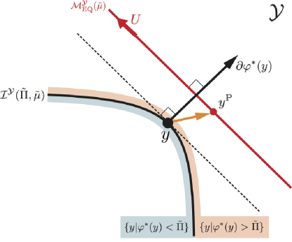
The vector represents a gradient of the convex function , which is a normal vector at a point of the level set . Note that the orientation of the normal vector points to the superlevel set (see Fig. 8). Also, is a vector from the point on the level set to the point . represents the inner product of the two vectors.
To investigate the sign of the inner product, we consider the tangent plane of the level set at the point (see the dashed line in Fig. 8). This plane divides the space of into two regions. If the orientations of the two vectors, and , point to the same side of the tangent plane, their inner product is positive. If they point to the opposite sides, the inner product is negative.
When , the equilibrium manifold is located in the superlevel set. In addition, the tangent plane at the point is parallel to . Then, we can find such that is located on the same side of the tangent plane with the orientation of the normal vector at the point (see Fig. 8). In such a case, the inner product between and is positive for . Thus, exists such that .
Appendix K Proof of negative for any when
We show that, when , is negative for . Here, we assume that the stoichiometric matrix is productive, therefore, (see Appendix J).
Consider any point . At the point , we can consider the tangent plane of the level set , which divides the space of into two regions. Since represents the inner product of the two vectors and in Eq. (104), the sign of is determined from the sides of the tangent plane to which the two vectors point. We also note that any point is on the one side of the tangent plane because the plane is parallel to the equilibrium manifold (see Fig. 9).
When , the equilibrium manifold (the red line in Fig. 9) is located both in the sublevel and the superlevel sets. From the convexity of the function , any point in the sublevel set is located on the opposite side of the tangent plane to the orientation of the normal vector at the point (see Fig. 9). Since any point is on the one side of the tangent plane, we can show that the particular solution is located on the opposite side of the tangent plane to the orientation of . Thus, for , the inner product between and is negative. Therefore, for , is always negative.
Appendix L Symbols and Notations
| Symbol | Description/definition | First appearance |
|---|---|---|
| The number of confined chemicals ( = ). | Sec. II.1 | |
| The initial condition of | Sec. II.1/Eq. (4) | |
| The number of open chemicals ( = ) | Sec. II.1 | |
| The number of species of confined chemicals | Sec. II.1 | |
| The number of species of open chemicals | Sec. II.1 | |
| The energy of the CRS | Sec. II.1 | |
| The volume of the CRS | Sec. II.1 | |
| The chemical potential of open chemicals in the environment | Sec. II.1 | |
| The temperature of the environment | Sec. II.1 | |
| The pressure of the environment | Sec. II.1 | |
| The number of open chemicals in the environment | Sec. II.1 | |
| The energy of the environment | Sec. II.1 | |
| The volume of the environment | Sec. II.1 | |
| The entropy function for the CRS | Sec. II.1 | |
| The entropy function for the environment | Sec. II.1 | |
| The total entropy function | Sec. II.1/Eq. (1) | |
| The entropy density | Sec. II.1/Eq. (2) | |
| Sec. II.1 | ||
| The stoichiometric matrix for confined chemicals | Sec. II.1/Fig. 1 | |
| The stoichiometric matrix for open chemicals | Sec. II.1/Fig. 1 | |
| The chemical reaction flux ( = ). | Sec. II.1/Eq. (3) | |
| The number of reactions | Sec. II.1 | |
| The energy exchange rate with the environment | Sec. II.1/Fig. 1 | |
| The volume expansion rate | Sec. II.1/Fig. 1 | |
| The diffusion flux for open chemicals | Sec. II.1/Fig. 1 | |
| The extent of reaction | Sec. II.1/Eq. (4) | |
| The conserved quantities ( = ). | Sec. II.1/Eq. (6) | |
| A basis matrix whose row vectors form the basis of | Sec. II.1/Eq. (6) | |
| The conserved quantities under the condition | Sec. III.3 | |
| The partial grand potential density | Sec. II.1/Eq. (13) | |
| The Legendre dual variable of | Sec. II.2 | |
| The full grand potential density | Sec. II.2/Eq. (20) | |
| The minimum pressure that the CRS can take | Sec. III.1/Eq. (34) | |
| The thermodynamic force | Sec. V.2/Eq. (60) |
| Symbol | Description/definition | First appearance |
| The number space | Sec. II.1 | |
| The density space | Sec. II.1 | |
| The chemical potential space | Sec. II.2 | |
| The space of conserved quantities | Sec. II.1 | |
| The equilibrium manifold in | Sec. II.2/Eq. (23) | |
| The equilibrium manifold in | Sec. III.4/Eq.(51) | |
| The isobaric manifold in or | Sec. III.2/Eq. (37), Eq. (39) | |
| The stoichiometric manifold/compatibility class in , , or | Sec. II.3/Eq. (24)-(26) | |
| The stoichiometric manifold in or under the condition | Sec. III.3/Eq. (43), Eq. (44) | |
| A nonlinear function of defined as | Sec. II.1/Eq. (18) | |
| The corresponding ray to in the space | Sec. II.1/Eq. (19) | |
| The corresponding ray to in the space | Sec. II.2/Eq. (21) | |
| Eq. (28) | Sec. II.4 | |
| Sec. II.6/Fig. 2 | ||
| A particular solution to Eq. (50) | Sec. III.4/Eq. (53) | |
| A coordinate of | Sec. III.4/Eq. (53) | |
| The intersecting point | Sec. III.5/Theorem 1 | |
| For regular , . | Sec. II.5 | |
| Birch’s point | Sec. V.1/Eq. (55) | |
| Birch’s trajectory | Sec. V.1/Eq. (56) | |
| Eq. (62) | Sec. V.2 | |
| The Bregman divergence | Sec. V.2/Eq. (63) | |
| The extent of reaction at the boundary of the domain | Sec. V.2 | |
| Sec. V.2 | ||
| The index set such that | Sec. V.2 |
| Symbol | Description/definition | First appearance |
| The gas constant | Sec.II.1 | |
| The standard chemical potentials of confined chemicals | Sec.II.1 | |
| The standard chemical potentials of open chemicals | Sec.II.1 | |
| The density of open chemicals in the environment | Sec.II.1/Eq. (16) | |
| Fig. 2/Appendix B | ||
| Fig. 2/Appendix B | ||
| , | The rate constants of -th forward and backward reactions | Appendix B |
| , | The rate constants where we absorb the constant densities of open chemicals | Appendix B |