Thermal rectification in the one-dimensional nonlinearly graded rotor lattice robust in the thermodynamical limit
Abstract
Recently, it has been shown that in graded systems, thermal rectification (TR) effect may remain in the thermodynamical limit. Here, by taking the one-dimensional rotor lattice as an illustrating model, we investigate how the graded structure may affect the TR efficiency. In particular, we consider the case where the interaction is assigned with nonlinear polynomial functions. It is found that TR is robust in the thermodynamical limit and meanwhile its efficiency may considerably depend on the details of the graded structure. This finding suggests that it is possible to enhance the TR effect by taking into account the nonlinear graded structure even in large systems.
I Introduction
Thermal rectification (TR) is an interesting heat transport phenomenon Starr1936 ; Peyrard2002 . In a system where TR takes place – such a system is termed as a thermal rectifier or a thermal diode – the heat current flows preferably along a particular direction than along the others. As such TR can be utilized to control and manage thermal flows, hopefully leading to the promising novel and exciting applications Modrev .
The study of TR is also of fundamental theoretical interest in revealing the basic transport properties. In this respect, since the pioneer work by Terraneo et al Peyrard2002 attempting to relate TR with the underlying microscopic dynamics, significant progress has been made. So far two necessary conditions for TR have been identified PeyrardEPL : One is the asymmetry in the system’s structure and another is the (sensitive) dependence of the local heat transport on the local structure and temperature. Based on this understanding, most of the ensuing research has devoted to identifying the various mechanisms that can magnify the structure asymmetry, e.g., by introducing the long range interactions SD2015 , or the dependence sensitivity of the local heat transport on the local structure and temperature, e.g., by taking advantage of the phase transition Kobayashi . The study along this line has turned out very successful and fruitful.
In spite of the progress achieved, however, there is an unsolved theoretical mystery. That is, for a lattice system, why, as the system size increases, does the TR effect usually decay and vanishe eventually in the thermodynamical limit ZhYPRL ? Intuitively, provided other conditions unchanged, when the system size is increased, the change rate of any relevant quantity along the system would decrease correspondingly, so that the effect of the structural asymmetry as well as the sensitive dependence of the local heat transport could be weakened. Given this, in order to retrieve TR in large systems, its two preconditions must be robust against the increase of the system size. From this consideration, two particular approaches have been proposed for maintaining TR in large systems. One is to employ the integrability, because for an integrable system, the heat current flowing across it does not depend on the system size Lepri2003 . An illustrating example is given in Ref. SD2018 , where it is shown that by introducing a harmonic (integrable) chain as a spacer into a thermal diode, TR keeps its efficiency in any long system as the length of the spacer can be set at will. Another interesting example consists of hard-point particles with graded masses, which is not exactly integrable but tends asymptotically to the integrable limit as the system size increases, where TR is found to hold its efficiency as well WJ2012 . The second approach is to take good advantage of the sensitive temperature dependence of the heat conduction. The one-dimensional rotor lattice RL85 ; RL87 serves as an enlightening example, where the sensitive temperature dependence could even be progressively enhanced in the thermodynamical limit RL-Livi ; RL-Savin ; RL-Spohn ; RL-Dhar . As a result, it is possible to design a graded rotor lattice whose TR efficiency could even keep increasing instead as the system size SJ2020 .
Note that this intriguing TR effect exhibited in the graded rotor lattice is due to the strong nonlinear effect of a transition RL-Livi ; RL-Savin ; RL-Spohn ; RL-Dhar . Even for a linearly graded lattice whose gradient decreases with the increasing system size, the strong nonlinear effect may manifest itself remarkably (e.g., as seen in the temperature profile SJ2020 ). It is therefore interesting to investigate how robust and sensitive is the underlying mechanism by which the nonlinear effect plays its role to result in TR. To probe it, we may turn to the executable question that is concerned with: If the linearly graded structure is perturbed, how the TR effect may respond. In previous studies, the linearly graded structure has been taken into account intensively and prevailingly, which might be out of the implicit assumption that the effect caused by the perturbation is negligible or trivial. Our motivation here is to study this issue by considering the perturbed graded rotor lattice, and as shown in the following, it is found that this assumption does not apply.
II Model and method
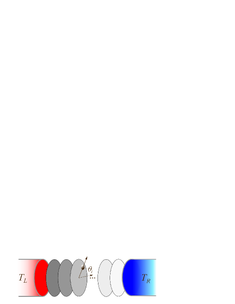
Our model system consists of rotors positioned on a one-dimensional lattice (see Fig. 1 for a schematic plot). We take the dimensionless units throughout, in which the lattice constant is unit and thus also measures the length (size) of the system. The Hamiltonian for a symmetric, homogeneous rotor lattice is RL85 ; RL87
| (1) |
where is the angular variable of the th rotor with respect to a given reference axis and the corresponding conjugate variable. The potential conventionally assumed is
| (2) |
where, in order to keep the maximum force between any two neighboring rotors a constant (set to unity) independent of the two parameters and , they are set to satisfy , so that is adopted as the only independent parameter SJ2020 .
In this homogeneous rotor lattice, a striking property is that there exists a transition temperature, , governed by the interaction strength, , below and above which the heat conduction is of ballistic and diffusive type, respectively, characterized accordingly by a divergent and convergent heat conductivity RL-Livi ; RL-Savin ; RL-Spohn ; RL-Dhar . Specifically, it has been established that approximately SJ2020 . As such we should be able to build a thermal diode by introducing the graded interaction strength to ensure that, when the heat current flows in the direction the interaction strength decreases, the local temperature keeps below the local transition temperature throughout, so that the current is strong. But when the current flows in the opposite direction, the local temperature is above the local transition temperature at the high temperature end, so that this part of the lattice plays an impeding role to resist the current. This idea has been verified to be valid SJ2020 . Specifically, for an interaction-strength graded rotor lattice, its Hamiltonian is still given by Eq. (1), but with the potential term being replace by the local interaction potential
| (3) |
where is fixed to be and specifies the local interaction strength. The local transition temperature thus reads as .
Without loss of generality, suppose that changes from to with and being two parameters satisfying . Moreover, we refer to the direction from left to right, i.e., from the first to the last rotor, the forward direction. For our aim here, we restrict ourselves to investigate the graded lattices whose local interaction strength is specified by the following cubic polynomial function:
| (4) |
i.e., we set the rescaled position of the th rotor as , and then the corresponding interaction strength is given as . The four coefficients are set by the “boundary” conditions that, at the two ends, and , and additionally, and , with the tangent and at the two ends respectively being two additional parameters for us to control the local interaction strength in between. The special case of the linearly graded lattice studied previously SJ2020 corresponds to , or equivalently, , and any other case can be seen as a perturbation to this special one. With the freedom to assign and , in the following we will scrutinize how the TR efficiency would change as and for a given pair of values of and with which the linearly graded lattice functions as a thermal diode. Surely, by considering polynomial functions of high order or other forms of functions would allow us to study more complicated and comprehensive perturbations; this will be discussed later.

Next, to measure the TR efficiency, we perform the molecular dynamics simulations. To this end, the system is coupled to two extra rotor lattice segments of and rotors (sizes), respectively, at its left and right sides. Besides the neighboring interactions the same as in the system but with homogeneous strength of and , the motion of the rotors in these two segments are also subject to the applied Langevin heat baths of temperature and , so that their motion equations are with being a white Gaussian noise satisfying that . Here governs the coupling strength between the rotor and the heat bath and is the Boltzmann constant (set to unity). For the system rotors in between these two segments, their motion equations are . With all the motion equations, the whole system is integrated numerically with a standard algorithm. When the system has relaxed into the stationary state, the heat current is measured as the time average of the local current , i.e., , where can be defined as Lepri2003 . To obtain the TR efficiency at a given working temperature with a given bias , let us denote the high and low boundary temperatures by and , respectively; the forward current is thus measured numerically by setting and and the reverse current by and . Then the TR efficiency can be measured as Walker
| (5) |
Here both and represent their absolute values. In our simulations, we have adopted the velocity-Verlet algorithm VV and set and , but it has been checked and verified that the results do not depend on these particular adoptions.
III Results
Now we are ready to present the simulation results. For our aim here, in the following we will focus on the typical case where , , , and . The linearly graded lattice with this set of parameter values has been found to be an ideal thermal diode whose TR efficiency keeps growing as the system size SJ2020 . With the setup detailed above, our particular interest is to reveal how the TR efficiency would change when and deviate from of the linearly graded lattice.
Our main results are summarized in Fig. 2, where the TR efficiency, the forward and reverse current, are presented as functions of and , respectively. For the sake of comparison, shown in Fig. 2 are the values rescaled by those of the linearly graded lattice, , , and , respectively; i.e., , , and . Note that in all three panels of Fig. 2, the center point () corresponds to the linearly graded lattice. Above all, as Fig. 2(a) shows, the TR efficiency has a by no means trivial dependence on and . Over the investigated range of and , may undergo a considerable variation up to about of . In particular, an increase as high as over of can be reached (see for and ), suggesting convincingly that the perturbation effect is worth considering to enhance TR. On the other hand, the perturbation may lower the TR efficiency as well. However, taking into account the information of the forward and the reverse current [see Figs. 2(b) and 2(c)], it may provide us with more flexibility for designing the thermal diode of certain functions. For example, if we take the values of and at the bottom-right corner, then the resultant thermal diode would have such a property that the forward current remains close to its maximum, whereas the TR efficiency is dominantly determined by the reverse current that depends on and much more sensitively. Of particular advantage is the area bounded by the two white dashed lines [see Fig. 2(a)], where not only the TR efficiency is higher than the linearly graded lattice, but also the forward current is stronger meanwhile the reverse current is weaker, respectively, than their counterparts in the latter.

In order to understand the perturbation effect emerges in Fig. 2, we study the temperature profiles of four representative cases (see Fig. 3). First, even for the linearly graded rotor lattice [see Fig. 3(a)], the temperature profile is obviously far from a straight line when the current flows reversely, in spite of the small, constant gradient of the local interaction strength, which is about in this case. The key role for forming such a curved temperature profile is played by the right end segment (the shaded part) where the local temperature is higher than the local transition temperature. As such the heat conduction is suppressed in this segment, making it an effective thermal insulator. As a result, the temperature drops rapidly over this segment. On the other hand, for the left segment, the local temperature is below the local transition temperature, and hence it serves instead as a thermal conductor, over which the temperature drop must be lower. This explains why the temperature profile for the reverse current is characterized, respectively, by two segments of a mild and a rapid change. From this analysis we can see that, as mentioned above, this strong nonlinear effect is indeed rooted in the transition. As to the forward current, the local temperature is below the local transition temperature throughout; therefore the whole lattice works as a thermal conductor, leading to a strong forward current as well as a roughly linear temperature profile.
Importantly, as indicated by other panels of Fig. 3, the mechanism of transition works generally even when the linearly graded structure is perturbed, showing that this mechanism is quite robust. Comparing the temperature profiles of all four cases, it can be seen that the difference between them is slight, implying that the system has a strong adaptive ability to stabilize the temperature profiles against the perturbation. In fact, the perturbations in the three perturbed cases are not very weak, which can be told directly from the curve that represents the local interaction strength as well due to . Indeed, for the three perturbed cases, the deviation of from the linearly graded rotor lattice is obvious. In addition, the robustness of the transition mechanism also reflects in the fact that the TR behavior in the perturbed cases can be explained based on the and temperature curves. For example, comparing Figs. 3(c) and 3(d), the temperature profile for the forward current (the red curve) lies much lower below in the former, suggesting that the forward current should be stronger in the former than in the latter, which is in agreement with the results in Fig. 2(b). Similarly, for the reverse current (the blue curve), as the resisting layer (shaded) is thicker in the latter, a weaker reverse current is therefore expected in the latter, agreeing with the result in Fig. 2(c). Due to these robustness features of the transition mechanism, it is interesting to note that the TR behavior of a perturbed graded rotor lattice can be qualitatively predicted without performing the simulations, because we can take the temperature profiles of the linearly graded rotor lattice as approximations, and compare them with the transition temperature curve for the given interaction strength .

As a crucial issue for our motivation here, we need to investigate if the robustness features addressed above would survive the thermodynamical limit. Our simulation results suggest a positive answer to this question. To this end, several representative cases are simulated with various system sizes, and the results for the TR efficiency are presented in Fig. 4. It can be seen that, accompanying with the curve for the linearly graded rotor lattice, all other curves for the illustrative perturbed cases keep to grow together. This property is welcomed; it shows that the perturbation effect is robust in the thermodynamical limit and hence may be utilized to improve the TR efficiency for any size of the system.

So far we have focused on the polynomial perturbation up to the cubic term for two reasons. One is that we have supposed such a form may have captured the most significant part of a perturbation. Another is that, as such we have two free parameters ( and ), the two-dimensional parameter space spanned by them has been big enough to explore in view of our computing resources, which have been fully engaged in carrying out a detailed investigation as in Fig. 2. But what effect a complicated perturbation may have is not clear yet, and it seems to be hard to predict in view of the strong nonlinear effect we have witnessed. Just as a preliminary attempt, we show in Fig. 5 how the TR efficiency may respond if the fourth-order term, , is added to the function given in Eq. (4), where, for a given value of , other four parameters are determined in the same way. Undoubtedly, as shown in Fig. 5, the effect it induces could be significant, justifying that more complicated perturbations deserve further study.
Finally, as a comparison, in the following we conduct a parallel study of the mass graded Fermi-Pasta-Ulam-Tsingou (FPUT) lattice FPU-1 ; FPU-2 . Its Hamiltonian is
| (6) |
where and are the conjugate variable pair of the th particle, its mass, and . The mass graded FPUT model was first come up with in Ref. YNPRB , where the TR was illustrated for the first time in the graded structure. Specifically, it is reported in Ref. YNPRB that when the masses of the particles of the system are assigned to change linearly from to , a relatively stronger TR effect would be observed at the working temperature with the system size .

As our simulation results suggest (see in the following), with the increasing size, the TR effect would decay till disappear. This is in clear contrast with the interaction-strength graded rotor lattice. Our motivation here is to see what the perturbation to the linearly graded structure may lead to in this category of TR systems. Similarly, in this case we set the graded masses of particles according to the cubic polynomial function of Eq. (4) as well; i.e., , where is the rescaled average position of the th particle. The four prefactors in are set following the conditions that , , , and . As such the case of linearly graded masses corresponds to , and we take it as the reference again. The working temperature and temperature bias are set to be . The simulation method and the related parameter values are the same as adopted in the simulations of the rotor lattice.
First, a counterpart of Fig. 2 but here for the mass graded FPUT lattice is presented as Fig. 6 for that ensures roughly the strongest TR efficiency. In Fig. 6(a), it can be recognized that, though more moderate than in the graded rotor lattice, the perturbation can still result in a significant change in the TR efficiency, from about below to above (corresponding to the center point), over the square range of and investigated. Therefore, even for this category of TR systems, there is still space for improving the TR effect by adapting the nonlinearly graded structure. On the other hand, such a study as in Fig. 6 may also help for revealing more features of the studied object. Taking the current case as an example, it shows [see Fig. 6(a)] that generally the TR efficiency has a more sensitive dependence on rather than , suggesting that the detailed mass distribution over the heavy end of the system could matter more.
Next, let us probe how the TR efficiency may vary versus the system size. The results for three representative cases are illustrated in Fig. 7. It is interesting to note that, as in the linearly mass graded case, in the perturbed cases the TR efficiency hits its maximum more or less around the size of as well. Moreover, the variant range or due to the perturbation is also the widest at the same size. Decreasing or increasing the system size, neither the TR nor the perturbation effect on TR would be sustained, indicating that neither is robust against the change of the system size.
IV Discussion and conclusions

In summary, we have investigated how the graded structure may influence TR with two paradigmatic lattice models as representatives of two distinct categories. We have mainly focused on the possible effect a perturbation to the linearly graded structure may induce. In terms of the TR efficiency, it has been found that, the perturbation effect depends on the TR efficiency of the linearly graded structure itself: The larger the TR efficiency in the latter, the larger the variation to it the perturbation may bring in. Therefore, for a good thermal diode, adaption of the graded structure may serve as an effective tactic to optimize its TR efficiency. Besides, the study from the perturbation perspective has also been found to be effective to reveal other interesting properties, such as the strong adaptive ability to maintain the temperature profiles in the graded rotor lattice.
In the present study, only the graded structures described by cubic polynomial functions are concerned. Though other graded structures are worth studying, the challenge of simulation has to be faced. In this respect, the machine learning technique may provide a powerful tool. Indeed, as illustrated in a series of recent studies, the machine learning method has been found superior in studies of thermal conduction issue (see Ref. ML for a recent review and references cited therein). Its advantage lies in that the brutal searching in the parameter space can be avoided; instead, aiming at the prescribed TR target, the learning machine may figure out the shortcuts to the target. For the TR effect that sustains in the thermodynamical limit, the structure of the known models, such as that with the integrable spacer and the graded rotor lattice, can be used as input for training. It would be rewarding if new mechanisms and models unknown yet can be solved out by this strategy.
This work is supported by the National Natural Science Foundation of China (Grants No. 12075198 and No. 12047501).
References
- (1) C. Starr, Physics 7, 15 (1936).
- (2) M. Terraneo, M. Peyrard, and G. Casati, Phys. Rev. Lett. 88, 094302 (2002).
- (3) N. Li, J. Ren, L. Wang, G. Zhang, P. Hänggi, and B. Li, Rev. Mod. Phys. 84, 1045 (2012).
- (4) M. Peyrard, Europhys. Lett. 76, 49 (2006).
- (5) S. Chen, E. Pereira, and G. Casati, Europhys. Lett. 111, 30004 (2015).
- (6) W. Kobayashi et al., Appl. Phys. Express 5, 027302 (2012).
- (7) B. Hu, L. Yang, and Y. Zhang, Phys. Rev. Lett. 97, 124302 (2006).
- (8) S. Lepri, R. Livi, and A. Politi, Phys. Rep. 377, 1 (2003).
- (9) S. Chen, D. Donadio, G. Benenti, and G. Casati, Phys. Rev. E. 97, 030101(R) (2018).
- (10) J. Wang, E. Pereira, and G. Casati, Phys. Rev. E 86, 010101(R) (2012).
- (11) G. Benettin, L. Galgani, and A. Giorgilli, Il Nuovo Cimento B 89, 89 (1985).
- (12) R. Livi, M. Pettini, S. Ruffo, and A. Vulpiani, J. Stat. Phys. 48, 539 (1987).
- (13) C. Giardiná, R. Livi, A. Politi, and M. Vassalli, Phys. Rev. Lett. 84, 2144 (2000).
- (14) O.V. Gendelman and A.V. Savin, Phys. Rev. Lett. 84, 2381 (2000).
- (15) H. Spohn, arXiv: 1411.3907v1.
- (16) S. G. Das and A. Dhar, arXiv: 1411.5247v2.
- (17) S. You, D. Xiong, and J. Wang, Phys. Rev. E 101, 012125 (2020).
- (18) N. A. Robert and D. G. Walker, Int. J. Thermal Sci. 50, 648 (2011).
- (19) M. P. Aüllen and D. L. Tildesley, Computer Simulation of Liquids (Clarendon, Oxford, 1987).
- (20) E. Fermi, J. Pasta, and S. Ulam, Los Alamos Report No. LA-1940, 1955.
- (21) T. Dauxois, Phys. Today 61, 55 (2008)
- (22) N. Yang, N. Li, L. Wang, and B. Li, Phys. Rev. B 76, 020301(R) (2007).
- (23) Y. Ouyang, C. Yu, G. Yan and J. Chen, Front. Phys. 16, 43200 (2021)