Thermal capillary waves on bounded nanoscale thin films

The free surface can be written as the superposition of the average film thickness $h_{0}$ and a perturbation $h_{1}(x,t)$:

$$h(x,t)=h_{0}+h_{1}(x,t).$$

(8)

Here, $h_{1}(x,t)$ can be decomposed into the wave modes $\phi_{n}(x)$, so that

$$h_{1}(x,t)=\sum_{n=1}^{\infty}a_{n}(t)\phi_{n}(x),$$

(9)

and it is assumed that $a_{n}(t)\ll h_{0}$. An energetic argument, exploiting equipartition in thermal equilibrium, will then give us the statistical properties of the amplitudes (the $a_{n}$’s).

The cost of energy for doing work against surface tension by expanding the interface’s area is given by

$$E=\gamma\left(L_{y}\int_{0}^{L_{x}}\sqrt{1+\left(\frac{\partial h}{\partial x}\right)^{2}}dx-L_{x}L_{y}\right),$$

(10)

where $L_{y}$ is the film length into the page. Taking the standard thin-film approximation that $\partial h/\partial x\ll 1$ we have

$$E\approx\gamma L_{y}\int_{0}^{L}\frac{1}{2}\left(\frac{\partial h}{\partial x}\right)^{2}dx,$$

(11)

so that using Eq. (8) and Eq. (9) we can obtain the total energy:

$$E=\sum_{n=1}^{\infty}E_{n}=\sum_{n=1}^{\infty}\frac{\gamma\pi^{2}n^{2}}{4}\frac{L_{y}}{L_{x}}a_{n}^{2}.$$

(12)

According to the equipartition theorem, at thermal equilibrium the energy is shared equally among each mode, i.e. $\langle E_{n}\rangle=k_{B}T/2$, leading to an expression for the variance of each mode’s amplitude (note their means are zero by construction):

$$\langle a_{n}^{2}\rangle=\frac{2}{\pi^{2}}l_{T}^{2}\frac{L_{x}}{L_{y}}\frac{1}{n^{2}}.$$

(13)

This expression then allows us to obtain information about the nanowaves in thermal equilibrium. Using Eq. (9) and $\langle a_{m}a_{n}\rangle=\delta_{mn}\langle a_{n}^{2}\rangle$ (see Appendix A.2), we can find the variance of the perturbation across the film as follows

	$\displaystyle\langle h_{1}^{2}(x)\rangle$	$\displaystyle=\left\langle\sum_{m=1}^{\infty}a_{m}\cos\left(\frac{m\pi x}{L_{x}}\right)\sum_{n=1}^{\infty}a_{n}\cos\left(\frac{n\pi x}{L_{x}}\right)\right\rangle$
		$\displaystyle=\sum_{n=1}^{\infty}\langle a_{n}^{2}\rangle\cos^{2}\left(\frac{n\pi x}{L_{x}}\right)$
		$\displaystyle=\frac{2l_{T}^{2}}{\pi^{2}}\frac{L_{x}}{L_{y}}\sum_{n=1}^{\infty}\frac{\cos^{2}\left(\frac{n\pi x}{L_{x}}\right)}{n^{2}}$
		$\displaystyle=l_{T}^{2}\frac{L_{x}}{L_{y}}\left[\frac{1}{12}+\left(\frac{1}{2}-\frac{x}{L_{x}}\right)^{2}\right].$		(14)

Notably, in contrast to the periodic spatially homogeneous case Eq. (4), expression Eq. (14) is a function of $x$. A full discussion of this case will be provided after we have compared to MD results.

There is also an alternative derivation for $\langle a_{n}^{2}\rangle$ directly from the STFE (see Appendix A.2). Since the STFE describes the time evolution of the film height from some initial (non-equilibrium) state, the result is also time dependent:

$$\langle a_{n}^{2}\rangle=\frac{2k_{B}T}{\gamma\pi^{2}}\frac{L_{x}}{L_{y}}\frac{1}{n^{2}}(1-\exp(-2An^{4}t)),$$

(15)

where $A=\gamma h_{0}^{3}\pi^{4}/(3\mu L_{x}^{4})$. This tells us that an initial perturbation decays exponentially with time, and that at thermal equilibrium (as $t\to\infty$) the results from the STFE agrees with Eq. (13) derived from thermal-capillary-wave theory, which provides a more straight forward derivation.

To verify our new theoretical prediction, we use molecular dynamics simulations (MD) as a virtual experiment to probe the behavior of quasi-2D thin films that are bounded on both sides by solid walls with $90^{\circ}$ contact angles.

The simulations are performed in the open-source software LAMMPS [50], which has been widely used to study fluid phenomena at the nanoscale, e.g. [29, 35, 51, 52, 53, 54, 55, 56, 57, 58]

Argon is used as a fluid and Platinum is used for the solid walls. The interaction between particles are modeled using the conventional Lennard-Jones 12-6 potential

$$V(r_{ij})=4\epsilon_{AB}\left[\left(\frac{\sigma_{AB}}{r_{ij}}\right)^{12}-\left(\frac{\sigma_{AB}}{r_{ij}}\right)^{6}\right],$$

(16)

where $r_{ij}$ is the distance between atoms $i$ and $j$, $\epsilon_{AB}$ is the energy parameter representing the depth of potential wells and $\sigma_{AB}$ is the length parameter representing the effective atomic diameter. Here, $AB$ are different combinations of particle types; namely, fluid-fluid (ff), solid-solid (ss) and solid-fluid (sf). The simulation parameters are summarized in Table 1 with corresponding non-dimensional ‘MD values’ henceforth denoted with an asterisk (as one can see, energy is scaled with respect to $\epsilon_{f\!f}$, lengths with $\sigma_{f\!f}$ and mass with $m_{f}$). To obtain a $90^{\circ}$ contact angle, we set $\epsilon^{*}_{sf}=0.52$ and $\sigma_{sf}^{*}=0.8$. The position of solid particles are fixed to reduce computational cost. The timestep is set to $0.0085$ ps.

Transport properties of liquid Argon are measured under MD simulations, with parameters given by Table 1. Shear viscosity $\mu=2.44\times 10^{-4}$ kg/(ms) is calculated using the Green-Kubo method [59]:

$$\mu=\frac{V}{3k_{B}T}\sum\int_{0}^{\infty}\langle J_{pq}(t)J_{pq}(0)\rangle dt,$$

(17)

where $V$ is the volume, $J_{pq}$ are the components of the stress tensor and the sum accumulates three terms given by $pq$ ($=xy,yz,zx$). Note, only off-diagonal terms of the stress tensor are used, as shear viscosity is measured by the transport of momentum perpendicular to velocity. Surface tension $\gamma=1.52\times 10^{-2}$ N/m is calculated from the difference between the normal and tangential components of pressure tensor in a simple vapor-liquid-vapor system ($z$-direction) [60, 61]:

$$\gamma=\frac{1}{2}\int_{0}^{L_{z}}\left(P_{zz}(z)-\frac{1}{2}\left(P_{xx}(z)+P_{yy}(z)\right)\right)dz,$$

(18)

where $L_{z}$ is the length of the simulation box in the $z$-direction and $P_{xx}$, $P_{yy}$, $P_{zz}$, are the diagonal components of the pressure tensor.

To set up the MD simulation we use the following procedure: (i) a block of liquid Argon is created in a periodic box with dimension $(L_{x},L_{y},h_{0})$, density $\rho_{l}$ and is equilibrated for $5\times 10^{6}$ timesteps with NVT at temperature $T$, (ii) a block of vapor Argon is created in a periodic box with dimension $(L_{x},L_{y},3h_{0})$, density $\rho_{v}$ then equilibrated for $5\times 10^{6}$ timesteps with NVT at temperature $T$, (iii) Platinum walls are created with a face centered cubic structure (fcc) of density $\rho_{s}$, each wall has $5$ layers of Platinum atoms with thickness $0.872$ nm, the bottom wall then has dimension $(L_{x},L_{y},0.872)$ , (iv) the equilibrated liquid Argon is then place onto the bottom wall with a $0.17$ nm gap between the solid and the liquid (the gap results from the repulsive force in the Lennard-Jones potential and its thickness is found after equilibration) [40], (v) equilibrated vapor Argon is placed on the top. The MD simulation is then run with NVT at temperature $T$. Fig. 1 shows a snapshot of the MD simulation. Periodic boundary conditions are applied only in the $y$-direction. A reflective wall is applied at the top boundary.

In our simulations, the position of the liquid-vapor interface is determined using the number density and a binning technique see [31]. We first calculate the number density of each Argon particle using a cut-off radius of $3.5\sigma_{f\!f}$. Particles with number density above $0.5n^{*}$ are then defined as liquid particles and particles with number density below $0.5n^{*}$ are identified as vapor particles, where $n^{*}=0.83$ is the non-dimensional number density of a liquid Argon particle in the bulk. The simulation domain is uniformly divided into vertical bins and the position of the free surface in each bin is determined by taking the maximum of the heights of all liquid particles inside the bin. Here, we use bins with side length $1.5\sigma_{f\!f}$ in $x$ and $1.4\sigma_{f\!f}$ in $y$. As a result the free surface position is projected onto a $x-y$ mesh and expressed as a 2D array.

Three different film lengths are tested: Film 1 ($L_{x}=13.04$ nm), Film 2 ($L_{x}=25.99$ nm) and Film 3 ($L_{x}=51.29$ nm). The film width $L_{y}=2.94$ nm is chosen so that the MD simulation can be consider quasi-2D. The initial film height $h_{0}=4.85$ nm is chosen so that the film is relatively thin, but yet does not breakup due to disjoining pressure [10, 9, 29]. The equilibriation time $t_{e}$, i.e. the time taken for all the waves to fully develop from an initially flat interface, is estimated by Eq. (86), which is the characteristic time for the mode with the longest wavelength (and thus slowest growth) to develop; this varies with film length $L_{x}$. Multiple independent MD simulations (realizations) (Film 1: 10, Film 2: 10, Film 3: 20) are performed in parallel to reduce wall-clock simulation time. Data is gathered after $t_{e}$ every $4000$ timesteps and the free surface position is averaged in the $y$-direction, to provide $h=h(x,t)$ at each snapshot.

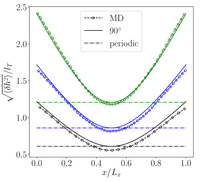
Fig. 2 shows the standard deviation of the free surface fluctuations, normalized by the thermal length scale $l_{T}$, obtained from MD simulations and compared to our theoretical predictions, Eq. (14); the agreement is excellent. The fluctuation amplitudes of an unbounded film (i.e. adopting a periodic boundary condition, Eq. (4)) are also provided. The relative strength of thermal fluctuations of the film interface increase with film length, as expected [19, 28]. However, comparing to Eq. (4) we can see that our expression predicts an enhanced fluctuation amplitude to that of a periodic film everywhere except at the center, $x=L_{x}/2$, where they coincide. Physically, this is because the replacement of periodicity with a fixed contact angle permits additional (‘half’) wave modes, i.e. of the form $\cos((2n-1)\pi x/L_{x})$ for $n=1,2,...$, which contribute to a larger amplitude everywhere except at $x=L_{x}/2$, where they are zero. Another interesting observation is that the effects of boundaries propagate across the whole film, regardless of the film length.

For a perfectly pinned contact line, the appropriate wave modes (see Appendix B.1) are

	$\displaystyle\varphi_{n}(x)$		$\displaystyle=\sinh(\lambda_{n}^{1/4}x)+\sin(\lambda_{n}^{1/4}x)$		(24)
			$\displaystyle+K\big{(}\cosh(\lambda_{n}^{1/4}x)-\cos(\lambda_{n}^{1/4}x)\big{)}$

with eigenvalues

$$\lambda_{n}\approx\left(\frac{\pi/2+n\pi}{L_{x}}\right)^{4},\qquad n=1,2,\ldots$$

(25)

As distinct from the $90^{\circ}$-contact-angle case, the mode corresponding to the $\lambda_{0}=0$ case also exists:

$$\varphi_{0}(x)=x\left(1-\frac{x}{L_{x}}\right).$$

(26)

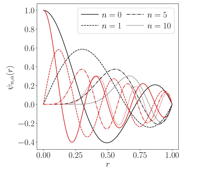
Although $\varphi_{n}(x)$ are not orthogonal, for odd $n$ they are odd functions around $x=L_{x}/2$ and for even $n$ they are even functions around $x=L_{x}/2$. We will exploit this property to simplify the calculation for fluctuation amplitudes later on. Figure 3 provides an illustration of $\varphi_{n}(x)$.

The partially-pinned-contact-line boundary condition is a linear combination of the perfectly pinned condition and the Langevin diffusion condition. This suggests that under linearization the free surface can be decomposed as

$$h(x,t)=h_{0}+h_{2}(x,t)+h_{3}(x,t),$$

(27)

where $h_{0}$ is the initial position of the contact line and $h_{2}(x,t)$, $h_{3}(x,t)$ are small perturbations. Applying this to Eq. (2), at the leading order ($h_{2}\sim h_{3}\sim\mathcal{N}\ll h_{0}$) we obtain

$$\frac{\partial h_{2}}{\partial t}+\frac{\partial h_{3}}{\partial t}=-\frac{\gamma h_{0}^{3}}{3\mu}\left(\frac{\partial^{4}h_{2}}{\partial x^{4}}+\frac{\partial^{4}h_{3}}{\partial x^{4}}\right)+\sqrt{\frac{2k_{B}Th_{0}^{3}}{3\mu L_{y}}}\frac{\partial\mathcal{N}}{\partial x}$$

(28)

and the boundary conditions in Eq. (6) and Eq. (19) become

	$\displaystyle h_{2}(0,t)$	$\displaystyle+h_{3}(0,t)=N_{1}(t),$		(29)
	$\displaystyle h_{2}(L_{x},t)$	$\displaystyle+h_{3}(L_{x},t)=N_{2}(t),$		(30)
	$\displaystyle\frac{\partial^{3}h_{2}}{\partial x^{3}}(0,t)$	$\displaystyle+\frac{\partial^{3}h_{3}}{\partial x^{3}}(0,t)=0,$		(31)
	$\displaystyle\frac{\partial^{3}h_{2}}{\partial x^{3}}(L_{x},t)$	$\displaystyle+\frac{\partial^{3}h_{3}}{\partial x^{3}}(L_{x},t)=0.$		(32)

This is actually a linear combination of two smaller problems, one with a noise-driven bulk and pinned contact lines

	$\displaystyle\frac{\partial h_{2}}{\partial t}=-\frac{\gamma h_{0}^{3}}{3\mu}\frac{\partial^{4}h_{2}}{\partial x^{4}}+\sqrt{\frac{2k_{B}Th_{0}^{3}}{3\mu L_{y}}}\frac{\partial\mathcal{N}}{\partial x},$		(33a)
	$\displaystyle h_{2}(0,t)=h_{2}(L_{x},t)=0,$		(33b)
	$\displaystyle\frac{\partial^{3}h_{2}}{\partial x^{3}}(0,t)=\frac{\partial^{3}h_{2}}{\partial x^{3}}(L_{x},t)=0,$		(33c)

and the other with deterministic equations in the bulk and noise-driven contact lines

	$\displaystyle\frac{\partial h_{3}}{\partial t}=-\frac{\gamma h_{0}^{3}}{3\mu}\frac{\partial^{4}h_{3}}{\partial x^{4}},$		(34a)
	$\displaystyle h_{3}(0,t)=N_{1}(t),\>h_{3}(L_{x},t)=N_{2}(t),$		(34b)
	$\displaystyle\frac{\partial^{3}h_{3}}{\partial x^{3}}(0,t)=\frac{\partial^{3}h_{3}}{\partial x^{3}}(L_{x},t)=0.$		(34c)

We can then solve Eqs. (33) for $h_{2}(x,t)$ by decomposing it into wave modes $\varphi_{n}(x)$

$$h_{2}=\sum_{n=1}^{\infty}c_{n}(t)\varphi_{n}(x),$$

(35)

where $c_{n}(t)$ are wave amplitudes that can be expressed explicitly (see Appendix B.2). Similarly $h_{3}(x,t)$ can also be decomposed into wave modes $\varphi_{n}(x)$ and boundary modes,

	$\displaystyle h_{3}(x,t)$	$\displaystyle=\sum_{n=1}^{N}e_{n}(t)\varphi_{n}(x)$
		$\displaystyle+N_{1}(t)\left(1-\frac{x}{L_{x}}\right)\left(1-\frac{x}{L_{x}}-u_{10}\frac{x}{L_{x}}\right)$
		$\displaystyle+N_{2}(t)\frac{x}{L_{x}}\left[\frac{x}{L_{x}}-u_{20}\left(1-\frac{x}{L_{x}}\right)\right].$		(36)

where $e_{n}(t)$ are wave amplitudes with explicit expressions, and $u_{10}$ and $u_{20}$ are constants that are given in Appendix B.3. Note, only $N$ wave modes are considered for $h_{3}(x,t)$, opposed to infinitely many wave modes considered for $h_{2}(x,t)$. This is because the wave modes are not orthogonal to each other, so when solving the linear system for $e_{n}(t)$, matrix $G$ is non-diagonal and it would be impossible to take its inverse if the dimension is infinite (see Appendix B.3). We can confirm numerically that this does not affect our results (the fluctuation amplitudes converge) and in Section IV we show that a cut-off on the number of wave modes is actually preferable.

We can obtain the fluctuation amplitude for $h_{2}$ using thermal-capillary-wave theory. Similar to the $90^{\circ}$-contact-angle case, we substitute Eq. (27) into Eq. (11) and use the fact that the $\partial\varphi_{n}/\partial x$ are orthogonal (see Appendix B.1) to obtain

$$E=\frac{\gamma L_{x}L_{y}}{2}\sum_{n=1}^{\infty}\lambda_{n}^{1/2}c_{n}^{2}+\hbox{other terms},$$

(37)

where the first term on the right hand is the change of surface area due to $h_{2}$ and the other terms are the change of surface area due to $h_{3}$ and cross terms of $h_{2}$ and $h_{3}$. Applying the equipartition theorem to the $h_{2}$ only terms we find

$$\langle c_{n}^{2}\rangle=l_{T}^{2}\frac{1}{L_{x}L_{y}}\frac{1}{\lambda_{n}^{1/2}}.$$

(38)

Using the fact that $\langle c_{m}c_{n}\rangle=\delta_{mn}\langle c_{n}^{2}\rangle$ (see Appendix B.2), finally, we have

$$\langle h_{2}^{2}(x)\rangle=l_{T}^{2}\frac{1}{L_{x}L_{y}}\sum_{n=1}^{\infty}\frac{\varphi_{n}^{2}(x)}{\lambda_{n}^{1/2}}.$$

(39)

Note, alternatively one can derive $\langle c_{n}^{2}\rangle$ directly from the STFE, which includes time dependence,

$$\langle c_{n}^{2}\rangle=\frac{k_{B}T}{\gamma}\frac{1}{L_{x}L_{y}}\frac{1}{\lambda^{1/2}}(1-\exp(-2C\lambda_{n}t)),$$

(40)

where $C=\gamma h_{0}^{3}/(3\mu)$ (see Appendix B.2). At thermal equilibrium this agrees with Eq. (38).

The fluctuations combine to give a total variance of

$$\langle(h_{2}+h_{3})^{2}\rangle=\langle h_{2}^{2}\rangle+2\langle h_{2}h_{3}\rangle+\langle h_{3}^{2}\rangle.$$

(41)

where $\langle h_{2}^{2}\rangle$ is the fluctuation of the bulk, already calculated via thermal-capillary-wave theory, and $\langle h_{3}^{3}\rangle$ is the fluctuation of the film originating from fluctuations of the contact lines. Notably, since the random variables $\mathcal{N}(x,t)$, $f_{1}(t)$ and $f_{2}(t)$ are uncorrelated, $\langle h_{2}h_{3}\rangle=0$ (see Appendix B.4). An expression for $\langle h_{3}^{2}(x)\rangle$, obtained from Eq. (187), can be found in Appendix B.4.

The MD simulations are the same as in Section II.1.2 with the exception that we need to pin the contact line. There are several ways to achieve this, for example, by using topographical defects on the solid substrate [65], but here we use the technique described by Kusudo et. al [66] using chemical heterogeneity. As shown in Fig. 4, this is achieved by using a hydrophilic wall (blue) beneath the film’s equilibrium height ($h_{0}$) and a hydrophobic one (red), which is less wettable, above it. The wettability of the walls are tuned by changing the interaction parameters between solid and liquid, $\epsilon_{sf1}$ and $\epsilon_{sf2}$ [51]. This results in the position of the contact line following a Gaussian distribution with mean $h_{0}$, when in thermal equilibrium, as can be seen from Fig. 4 (d). The variance depends on the equilibrium contact angles (i.e. on the $\epsilon_{sf}$’s) of the walls and a small variance is preferable to mimic perfect pinning. Our choice of parameters are shown in Table 2.

Four different film lengths are tested: Film 4 ($L_{x}=13.04$ nm), Film 5 ($L_{x}=25.99$ nm), Film 6 ($L_{x}=51.29$ nm) and Film 7 ($L_{x}=102.30$ nm). The film width $L_{y}=2.94$ nm and the initial film height $h_{0}=4.85$ nm are the same as in the $90^{\circ}$-contact-angle case. The equilibration time $t_{c}$ can be estimated from Eq. (107). Multiple independent MD simulations are performed (Film 4: $18$, Film 5: $10$, Film 6: $10$ and Film 7: $20$).

Fig. 5(a) shows the fluctuation amplitudes of the free surface obtained from MD simulations using bins with side length $1.5\sigma_{f\!f}$ in the $x$-direction and $1.4\sigma_{f\!f}$ in the $y$-direction, which agree well with the theoretical predictions, Eq. (41). Notably, the largest difference between the MD and theory occurs for the shortest films; an effect we will revisit in Section IV. One can see that the fluctuation amplitudes of films with partially pinned contact lines have a saddle shape with one trough and two crests, symmetric about $x=L_{x}/2$ as we would expect. In contrast to the previous case of a fixed contact angle, here the fluctuations are almost everywhere lower than those for a periodic film. The amplitudes dip significantly at the wall, due to the pinning effect, but do not reach zero due to the oscillations around the pinning position. Moreover, the positions of the trough and the crests relative to the length of the film are fixed, showing again that the boundary effects propagate across the film. Lastly, as suggested by our theory Eq. (41), the fluctuation amplitudes of the free surface can be attributed to the thermal noise in the bulk $\sqrt{\langle h_{2}^{2}\rangle}$ and the fluctuations of the contact line $\sqrt{\langle h_{3}^{3}\rangle}$. From the decomposition of fluctuation amplitudes shown in Fig. 5 (b) one can see that the effect of contact line fluctuations is limited to the region near the boundaries and clearly in this regime the bulk fluctuations are stronger than the contact-line-driven motions.

The free surface can be written in terms of the wave modes:

$$h(r,\theta,t)=h_{0}+h_{4}(r,\theta,t),$$

(54)

where the perturbation $h_{4}$ is

	$\displaystyle h_{4}(r,\theta,t)=\sum_{n=0}^{\infty}\sum_{\alpha=1}^{\infty}$	$\displaystyle\Big{[}A_{n,\alpha}(t)\Upsilon^{1}_{n,\alpha}(r,\theta)$
		$\displaystyle+B_{n,\alpha}(t)\Upsilon^{2}_{n,\alpha}(r,\theta)\Big{]}.$		(55)

Then we can calculate the energy of a perturbed surface (see Appendix C.2)

	$\displaystyle E$	$\displaystyle=\gamma\Bigg{(}\int_{0}^{2\pi}\int_{0}^{a}\sqrt{1+\left(\frac{\partial h}{\partial r}\right)^{2}+\frac{1}{r^{2}}\left(\frac{\partial h}{\partial\theta}\right)^{2}}rdrd\theta-\pi a^{2}\Bigg{)}$
		$\displaystyle\approx\frac{\gamma}{2}\int_{0}^{2\pi}\int_{0}^{a}\left(\left(\frac{\partial h}{\partial r}\right)^{2}+\frac{1}{r^{2}}\left(\frac{\partial h}{\partial\theta}\right)^{2}\right)rdrd\theta$
		$\displaystyle=\gamma\pi\sum_{\alpha=1}^{\infty}A_{0,\alpha}^{2}S_{0,\alpha}+\frac{\gamma\pi}{2}\sum_{n=1}^{\infty}\sum_{\alpha=1}^{\infty}(A_{n,\alpha}^{2}+B_{n,\alpha}^{2})S_{n,\alpha},$		(56)

where

$$S_{n,\alpha}=\frac{1}{2}(\omega_{n,\alpha}^{2}a^{2}-n^{2})J_{n}^{2}(\omega_{n,\alpha}a).$$

(57)

Since the wave modes are orthogonal to each other (see Appendix C.2) and the energy is quadratic in the amplitudes, we can use the equipartition theorem to give

$$\frac{k_{B}T}{2}=\gamma S_{0,\alpha}\langle A_{0,\alpha}^{2}\rangle$$

(58)

and

$$\frac{k_{B}T}{2}=\frac{\gamma\pi}{2}S_{n,\alpha}\langle A_{n,\alpha}^{2}\rangle=\frac{\gamma\pi}{2}S_{n,\alpha}\langle B_{n,\alpha}^{2}\rangle,$$

(59)

so that the (position-dependent) variance of fluctuations is given by

	$\displaystyle\langle h_{4}^{2}(r,\theta)\rangle$	$\displaystyle=\frac{k_{B}T}{\gamma}\frac{1}{\pi}\Big{[}\sum_{\alpha=1}^{\infty}\frac{1}{2S_{0,\alpha}}\chi_{0,\alpha}^{2}(r)$
		$\displaystyle+\sum_{n=1}^{\infty}\sum_{\alpha=1}^{\infty}\frac{1}{S_{n,\alpha}}\chi_{n,\alpha}^{2}(r)\Big{]}.$		(60)

Note that the variance is only $r$ dependent, since periodicity in $\theta$ eliminates variations.

Asymptotic analysis shows that $S_{n,\alpha}$ increases with $n$ linearly (see Appendix C.2). So the summation over $n$ in Eq. (60) diverges as $n\to\infty$ and a cut-off for smallest length scale $\ell_{c}$ should be introduced, as we’ve already seen for the periodic (i.e. unbounded) 3D film Eq. (46).

Applying a cut-off length scale in polar coordinates is non-trivial, as the modes in the $r$ and the $\theta$ directions differ, in contrast to the Cartesian case, and the radial wavemodes have non-trivial form. To do so, we define the length scale of a wave mode $f_{n,\alpha}(r,\theta)$ as

$$\mathcal{L}(f_{n,\alpha})=\frac{\max_{r\in[0,a],\theta\in[0,2\pi]}|f_{n,\alpha}(r,\theta)|}{\max_{r\in[0,a],\theta\in[0,2\pi]}\left|\nabla f_{n,\alpha}(r,\theta)\right|},$$

(61)

where $||$ is the absolute value and $\nabla$ is the gradient operator. For simplicity, we denote the length scale of the wave mode for the $90^{\circ}$-contact-angle case as $L^{90}_{n,\alpha}=\mathcal{L}(\Upsilon^{1}_{n,\alpha})$, and one can easily check that $\mathcal{L}(\Upsilon^{1}_{n,\alpha})=\mathcal{L}(\Upsilon^{2}_{n,\alpha})$. We then introduce a threshold function

$$Z^{90}(\ell_{c},n,\alpha)=\begin{cases}1,&\text{ if }L_{n,\alpha}^{90}\geq\ell_{c}\\ 0,&\text{ if }L_{n,\alpha}^{90}<\ell_{c}\end{cases},$$

(62)

to identify wave modes with length scale greater than a chosen $\ell_{c}$. Finally, we apply the cut-off to Eq. (60)

	$\displaystyle\langle h_{4}^{2}(r,\theta)\rangle$	$\displaystyle=\frac{k_{B}T}{\gamma}\frac{1}{\pi}\Big{[}\sum_{\alpha=1}^{\infty}\frac{Z^{90}(\ell_{c},0,\alpha)}{2S_{0,\alpha}}\chi_{0,\alpha}^{2}(r)$
		$\displaystyle+\sum_{n=1}^{\infty}\sum_{\alpha=1}^{\infty}\frac{Z^{90}(\ell_{c},n,\alpha)}{S_{n,\alpha}}\chi_{n,\alpha}^{2}(r)\Big{]}$		(63)

which regularizes the unbounded sum. The effect of cut-offs will be further discussed in Section IV.

References

- Bocquet and Charlaix [2010] L. Bocquet and E. Charlaix, Chem. Soc. Rev. 39, 1073 (2010).
- Craighead [2006] H. Craighead, Nature 442, 387 (2006).
- Karnik et al. [2005] R. Karnik, R. Fan, M. Yue, D. Li, P. Yang, and A. Majumdar, Nano Letters 5, 943 (2005).
- Basaran et al. [2013] O. A. Basaran, H. Gao, and P. P. Bhat, Annual Review of Fluid Mechanics 45, 85 (2013).
- Lokesh et al. [2018] M. Lokesh, S. K. Youn, and H. G. Park, Nano Letters 18, 6679 (2018).
- Kavokine et al. [2021] N. Kavokine, R. R. Netz, and L. Bocquet, Annual Review of Fluid Mechanics 53, 377 (2021).
- Weinstein and Ruschak [2004] S. J. Weinstein and K. J. Ruschak, Annual Review of Fluid Mechanics 36, 29 (2004), https://doi.org/10.1146/annurev.fluid.36.050802.122049 .
- Kumar [2015] S. Kumar, Annual Review of Fluid Mechanics 47, 67 (2015).
- Craster and Matar [2009] R. V. Craster and O. K. Matar, Reviews of Modern Physics 81, 1131 (2009).
- Oron et al. [1997] A. Oron, S. H. Davis, and S. G. Bankoff, Reviews of Modern Physics 69, 931 (1997).
- Myers [1998] T. G. Myers, SIAM Review 40, 441 (1998).
- Bonn et al. [2009] D. Bonn, J. Eggers, J. Indekeu, J. Meunier, and E. Rolley, Reviews of Modern Physics 81, 739 (2009).
- Becker et al. [2003] J. Becker, G. Grün, R. Seemann, H. Mantz, K. Jacobs, K. R. Mecke, and R. Blossey, Nature Materials 2, 59 (2003).
- Sharma [2003] A. Sharma, The European Physical Journal E - Soft Matter 12, 397 (2003).
- Alizadeh Pahlavan et al. [2018] A. Alizadeh Pahlavan, L. Cueto-Felgueroso, A. E. Hosoi, G. H. McKinley, and R. Juanes, Journal of Fluid Mechanics 845, 642 (2018).
- Fetzer et al. [2007] R. Fetzer, M. Rauscher, R. Seemann, K. Jacobs, and K. Mecke, Physical Review Letters 99, 114503 (2007).
- Mandelstam [1913] L. Mandelstam, Annalen der Physik 346, 609 (1913).
- Bouchiat and Meunier [1971] M. A. Bouchiat and J. Meunier, J. Phys. France 32, 561 (1971).
- Vink et al. [2005] R. L. C. Vink, J. Horbach, and K. Binder, The Journal of Chemical Physics 122, 134905 (2005).
- Bouchiat and Meunier [1969] M. A. Bouchiat and J. Meunier, Physical Review Letters 23, 752 (1969).
- Aarts [2004] D. G. A. L. Aarts, Science 304, 847 (2004).
- Derks et al. [2006] D. Derks, D. G. A. L. Aarts, D. Bonn, H. N. W. Lekkerkerker, and A. Imhof, Physical Review Letters 97, 038301 (2006).
- Li et al. [2001] M. Li, A. Tikhonov, D. Chaiko, and M. Schlossman, Physical Review Letters 86, 5934 (2001).
- Hu et al. [2006] X. Hu, Z. Jiang, S. Narayanan, X. Jiao, A. R. Sandy, S. K. Sinha, L. B. Lurio, and J. Lal, Physical Review E 74, 010602 (2006).
- Alvine et al. [2012] K. J. Alvine, Y. Dai, H. W. Ro, S. Narayanan, A. R. Sandy, C. L. Soles, and O. G. Shpyrko, Physical Review Letters 109, 207801 (2012).
- Zhang et al. [2021a] Z. Zhang, Y. Wang, Y. Amarouchene, R. Boisgard, H. Kellay, A. Würger, and A. Maali, Physical Review Letters 126, 174503 (2021a).
- Koplik et al. [1988] J. Koplik, J. R. Banavar, and J. F. Willemsen, Physical Review Letters 60, 1282 (1988).
- Delgado-Buscalioni et al. [2008] R. Delgado-Buscalioni, E. Chacon, and P. Tarazona, Physical Review Letters 101, 106102 (2008).
- Zhang et al. [2019] Y. Zhang, J. E. Sprittles, and D. A. Lockerby, Physical Review E 100, 023108 (2019).
- Zhang et al. [2021b] Y. Zhang, D. A. Lockerby, and J. E. Sprittles, Langmuir 37, 8667 (2021b).
- Zhang et al. [2021c] Y. Zhang, J. E. Sprittles, and D. A. Lockerby, Journal of Fluid Mechanics 915, 10.1017/jfm.2021.164 (2021c).
- Thakre et al. [2008] A. K. Thakre, J. T. Padding, W. K. den Otter, and W. J. Briels, The Journal of Chemical Physics 129, 044701 (2008).
- Willis and Freund [2010] A. M. Willis and J. B. Freund, Physics of Fluids 22, 022002 (2010).
- Moseler and Landman [2000] M. Moseler and U. Landman, Science 289, 1165 (2000).
- Zhao et al. [2019] C. Zhao, J. E. Sprittles, and D. A. Lockerby, Journal of Fluid Mechanics 861, 10.1017/jfm.2018.950 (2019).
- Zhao et al. [2020] C. Zhao, D. A. Lockerby, and J. E. Sprittles, Physical Review Fluids 5, 044201 (2020).
- Perumanath et al. [2019] S. Perumanath, M. K. Borg, M. V. Chubynsky, J. E. Sprittles, and J. M. Reese, Physical Review Letters 122, 104501 (2019).
- Perumanath et al. [2020] S. Perumanath, M. K. Borg, J. E. Sprittles, and R. Enright, Nanoscale 12, 20631 (2020).
- Pothier and Lewis [2012] J.-C. Pothier and L. J. Lewis, Physical Review B 85, 115447 (2012).
- Zhang et al. [2020] Y. Zhang, J. E. Sprittles, and D. A. Lockerby, Physical Review E 102, 053105 (2020).
- Landau et al. [1995] L. D. Landau, E. M. Lifshits, and L. D. Landau, Fluid Mechanics, 2nd ed., Course of Theoretical Physics No. vol.6 (Butterworth-Heinemann, Oxford, 1995).
- Davidovitch et al. [2005] B. Davidovitch, E. Moro, and H. A. Stone, Physical Review Letters 95, 244505 (2005).
- Grün et al. [2006] G. Grün, K. Mecke, and M. Rauscher, Journal of Statistical Physics 122, 1261 (2006).
- Pedersen et al. [2019] C. Pedersen, J. F. Niven, T. Salez, K. Dalnoki-Veress, and A. Carlson, Physical Review Fluids 4, 124003 (2019).
- Mecke and Rauscher [2005] K. Mecke and M. Rauscher, Journal of Physics: Condensed Matter 17, S3515 (2005).
- Zhao et al. [2022] C. Zhao, J. Liu, D. A. Lockerby, and J. E. Sprittles, Physical Review Fluids 7, 024203 (2022).
- Shah et al. [2019] M. S. Shah, V. van Steijn, C. R. Kleijn, and M. T. Kreutzer, Journal of Fluid Mechanics 876, 1090 (2019).
- Durán-Olivencia et al. [2019] M. A. Durán-Olivencia, R. S. Gvalani, S. Kalliadasis, and G. A. Pavliotis, Journal of Statistical Physics 174, 579 (2019).
- Grant and Desai [1983] M. Grant and R. C. Desai, Physical Review A 27, 2577 (1983).
- Thompson et al. [2022] A. P. Thompson, H. M. Aktulga, R. Berger, D. S. Bolintineanu, W. M. Brown, P. S. Crozier, P. J. in ’t Veld, A. Kohlmeyer, S. G. Moore, T. D. Nguyen, R. Shan, M. J. Stevens, J. Tranchida, C. Trott, and S. J. Plimpton, Computer Physics Communications 271, 108171 (2022).
- Fernández-Toledano et al. [2019a] J.-C. Fernández-Toledano, T. D. Blake, and J. De Coninck, Journal of Colloid and Interface Science 540, 322 (2019a).
- Fernández-Toledano et al. [2019b] J. C. Fernández-Toledano, T. D. Blake, L. Limat, and J. De Coninck, Journal of Colloid and Interface Science 548, 66 (2019b).
- Chacón et al. [2014] E. Chacón, E. M. Fernández, and P. Tarazona, Physical Review E 89, 042406 (2014).
- Nguyen et al. [2014a] T. D. Nguyen, J.-M. Y. Carrillo, M. A. Matheson, and W. M. Brown, Nanoscale 6, 3083 (2014a).
- Wang and Wu [2015] F. Wang and H. Wu, Scientific Reports 5, 17521 (2015).
- Wen et al. [2021] J. Wen, D. Dini, H. Hu, and E. R. Smith, Physics of Fluids 33, 072012 (2021).
- Theodorakis et al. [2021] P. E. Theodorakis, A. Amirfazli, B. Hu, and Z. Che, Langmuir 37, 4248 (2021).
- Nguyen et al. [2014b] T. D. Nguyen, M. Fuentes-Cabrera, J. D. Fowlkes, and P. D. Rack, Physical Review E 89, 032403 (2014b).
- Haile et al. [1993] J. M. Haile, I. Johnston, A. J. Mallinckrodt, and S. McKay, Computers in Physics 7, 625 (1993).
- Trokhymchuk and Alejandre [1999] A. Trokhymchuk and J. Alejandre, The Journal of Chemical Physics 111, 8510 (1999).
- Smith et al. [2016] E. R. Smith, E. A. Müller, R. V. Craster, and O. K. Matar, Soft Matter 12, 9604 (2016).
- Nadkarni and Garoff [1992] G. D. Nadkarni and S. Garoff, Europhysics Letters (EPL) 20, 523 (1992).
- Schäffer and Wong [1998] E. Schäffer and P.-z. Wong, Physical Review Letters 80, 3069 (1998).
- van Kampen and Van Kampen [2007] N. G. van Kampen and N. G. Van Kampen, Stochastic Processes in Physics and Chemistry (Elsevier Science & Technology, Amsterdam, NETHERLANDS, THE, 2007).
- Gleason and Putnam [2014] K. Gleason and S. A. Putnam, Langmuir 30, 10548 (2014).
- Kusudo et al. [2019] H. Kusudo, T. Omori, and Y. Yamaguchi, The Journal of Chemical Physics 151, 154501 (2019).
- Morrison [2013] F. A. Morrison, An Introduction to Fluid Mechanics (Cambridge University Press, 2013).
- Flekkøy and Rothman [1995] E. G. Flekkøy and D. H. Rothman, Physical Review Letters 75, 260 (1995).
- Flekkøy and Rothman [1996] E. G. Flekkøy and D. H. Rothman, Physical Review E 53, 1622 (1996).
- Courant and Hilbert [2009] R. Courant and D. Hilbert, Methods of Mathematical Physics. Vol.1, Vol. 1 (Wiley-VCH, Weinheim, 2009).
- [71] W. R. Inc., Mathematica, Version 13.1.