THERMAL AND MAGNETIC FIELD STRUCTURE OF NEAR EQUATORIAL CORONAL HOLES
Abstract
We use full-disk, SOHO/EIT 195 calibrated images to measure latitudinal and day to day variations of area and average photon fluxes of the near equatorial coronal holes. In addition, energy emitted by the coronal holes with their temperature and strength of magnetic field structures are estimated. By analyzing data of 2001-2008, we find that variations of average area (A), photon flux (F), radiative energy (E) and temperature (T) of coronal holes are independent of latitude. Whereas inferred strength of magnetic field structure of the coronal holes is dependent on the latitudes and varies from low near the equator to high near both the poles. Typical average values of estimated physical parameters are: K. Average strength of magnetic field structure of coronal hole at the corona is estimated to be Gauss. If coronal holes are anchored in the convection zone, one would expect they should rotate differentially. Hence, thermal wind balance and isorotation of coronal holes with the solar plasma implies the temperature difference between the equator and both the poles. Contrary to this fact, variation of thermal structure of near equatorial coronal holes is independent of latitude leading to a conclusion that coronal holes must rotate rigidly that are likely to be anchored initially below the tachocline confirming our previous study (ApJ, 763, 137, 2013).
1 INTRODUCTION
Coronal holes (CH), with unipolar magnetic field structures (Harvey & Sheeley 1979; Harvey et al. 1982), are the lowest density plasma structures mainly detected in either UV or X-ray radiations of the sun’s atmosphere and are associated with rapidly expanding magnetic fields and the acceleration of the high-speed solar wind (Krieger et al. 1973; Neupert & Pizzo, 1974; Nolte et al. 1976; Zirker 1977; Cranmer 2009 and references therein; Wang 2009; Wiegelmann, Thalmann, Solanki 2014). Possible link of sunspot (Hiremath and Mandi 2004 and references there in; Hiremath 2009) activity on the Earth’s atmosphere and climate are well recorded in the literature. Recently, evidences are building up that coronal holes also trigger responses in the Earth’s upper atmosphere and magnetosphere (Soon et al. 2000; Lei et al. 2008; Shugai et al. 2009; Sojka et al. 2009; Choi et al. 2009; Ram, Liu & Su 2010; Krista 2011; Verbanac et al. 2011; Fathy et.al. 2014; Machiya and Akasofu 2014). Very recently, Hiremath, Hegde and Soon (2015) came to a conclusion that, in addition to influence of sunspots, emission of coronal holes also trigger and maintain Indian Monsoon rainfall.
From the ISRO (Indian Space Research Organization) funded project, authors′ interest in the study of coronal holes is to examine radiative responses of these structures on the Indian summer Monsoon rainfall. For this purpose, estimation of radiative flux and energy of the CH at 1 AU during their evolution passage on the solar disk is necessary. Keeping these main objectives in mind, by using SOHO/EIT 195 calibrated images, thermal structure of CH such as photon flux, energy and hence temperature at the sun and at 1 AU are estimated.
Dynamics such as rotation rates (Hiremath and Hegde 2013 and references there in) and in situ plasma conditions of the CH are also of considerable interest for the solar community as the fast solar wind most likely originates in these regions (Stucki et al. 2002; Hegde et.al. 2015). Ion temperatures in a polar coronal hole from the line width measurements are estimated by Tu et al. (1998). Centre-to-limb variation of radiance of the transition region and coronal lines have been obtained by Wilhelm et al. (1998). Doppler shifts measurements of CII, O VI and Ne VIII lines are obtained by Warren, Mariska and Wilhelm(1997). Peter & Judge (1999) also studied these and few other lines and found that the redshift to blue shift transition occurs at electron temperatures of about 5 K. Analysis of SXT/Yohkoh images (Hara et. al. 1996) have shown that the estimated temperature structure (1.8 -2.4 K) in CH is of same order as that in the ambient medium. Mogilevsky, Obridko and Shilova (1997) also arrive at a similar conclusion. From the analysis of Big Bear solar observatory magnetograms and SOHO EIT images, Zhang et.al. (2007) came to a conclusion that temperature of coronal hole and ambient medium is not entirely different.
In recent years, space based observations such as Yohkoh and SOHO missions are extensively used for estimation of temperature structure of CH (Hara et al. 1994; Moses et al. 1997). One physical parameter that senses thermal structure of CH is electron temperature that is estimated by different spectroscopic methods. A detailed assessment of observations in coronal holes and the deduced temperatures is published by Habbal, Esser and Arndt (1993). See also a detailed review of estimation of coronal hole temperature by Habbal (1996) and Wilhelm (2012) respectively. Electron temperatures in CH can be measured with the help of a Magnesium line ratio of a temperature-sensitive pair (see Wilhelm 2006). With the assumption that density and temperature of the gas from which spectral lines are formed are constant along the line of sight, Habbal et al. (1993) estimated the temperature structure of CH. Using two SOHO spectrometers, CDS and SUMER, electron temperature of CH is measured as a function of height above the limb in a polar coronal hole (David et al. 1998; Wilhelm et al. 1998). Doschek & Laming (2000) found that increase in the emission-line ratio of the polar coronal hole is primarily due to increase of the electron temperature with height. Marsch, Tu and Wilhelm (2000) found that the hydrogen temperature increased only slightly from 1 to 2 K in the height range from 12,000 to 18,000 km. Stucki et al. (2000) presented that with increasing formation temperature, spectral lines show on average, an increasingly stronger blue shift in coronal holes relative to the quiet sun at equal heliospheric angle. Furthermore, Xia, Marsch and Wilhelm (2004) reported that the bases of coronal holes seen in chromospheric spectral lines with relatively low formation temperatures displayed similar properties as normal quiet sun regions. More recently, studies of Wilhelm (2006; 2012) suggest that, in a polar coronal hole region, the electron temperature in plumes is estimated to be K and, K in the inter plume regions, at the height of 45 Mm above the limb.
From the silicon and iron coronal lines, Doscheck and Feldman (1977) conclude that CH temperature must be less than 1 MK. From the jets of coronal holes, Nistico et.al. (2011) compute electron temperature of CH by the filter ratio method at 171 and 195 and estimated the temperature structure with a magnitude in the range of 0.18-1.3 MK. By using two lines Mg IX (368 Å) and Mg X (625 Å) and, with a similar line ratio technique, Doyle et.al. (2010) derived the different coronal hole temperature structures during solar maximum ( 1.04 MK) and during minimum ( 0.82 MK) respectively. The EUV (Fe XV at 284 Å) and radio (at 169 and 408 MHz) observations (Chiuderi, Avignon and Thomas 1977) suggest that CH consists of a hot (10 % of the CH surface with K) and a cold ( K) regions to explain observations of both the EUV and radio coronal hole temperature structures. From the analysis of EUV (SOHO/CDS) and radio emission (164-410 MHz, by the Nancay Radioheliograph, France), and with a model, Chiuderi et. al. (1999) estimated the CH temperature structure to be K. From the spectroscopic diagnostics of Mg VIII (430.47 and 436.62 Å) ion, observed by Sky lab space probe, Dwivedi and Mohan (1995), estimated the coronal hole electron temperature to be K. Dwivedi, Mohan and Wilhelm (2000), from the SUMER observations, estimate the CH temperature to be K. Observations (Esser et.al. 1999) of Ly, 1216, Mg X (625 Å), and O VI (1038 Å) spectral lines with the UVCS instrument on board SOHO, from , yield that proton temperature of CH slowly increases between 1.35 and and does not exceed K in that region.
In most of the afore mentioned studies, estimated electron temperature, along the slit of the observations over the region of CH, does not represents temperature structure of whole CH. Using filter ratio technique, although one can use DEM method for estimation of temperature of CH, this method yields ambiguity (Zhang, White and Kundu, 1999; Landi, Reale & Testa 2012; Guennou et al. 2012). Moreover, line ratio method might not be appropriate ( see section 4.5, Slemzin, Goryaev and Kuzin 2014) for estimation of coronal hole temperature as there is a appreciable contribution of scattered light due to brighter ambient corona, especially for the coronal holes. However, in this study we present a simple method for estimation of radiative flux, energy and temperature structure of CH at the sun and near Earth.
As solar wind due to coronal hole is directly proportional to area (Hegde em et.al. 2015; Rotter et.al 2012; Karachik and Pevtsov 2011; Abramenko et. al. 2009; Shugai, Veselovsky and Trichtchenko 2009; Vršnak, Temmer and Veronig 2007; Nolte et.al. 1976), it is interesting to examine how these parameters vary during the evolution of coronal hole. To be specific, for example, as the Earth’s ionosphere responds with the solar wind due to coronal hole it is important to estimate physical parameters such as area, temperature structure, etc.,
As for dynamics, except some of the studies (Shelke & Pande 1985; Obridko & Shelting 1989; Navarro-Peralta & Sanchez-Ibarra 1994; Insley et al. 1995), other studies (Wagner 1975; Wagner 1976; Timothy & Krieger 1975; Bohlin 1977; Hiremath and Hegde 2013; Japaridze et.al. 2015) indicate rigid body rotation rates of the coronal holes. With large number of data and accurately estimated average longitude from the central meridian of the coronal holes, especially Hiremath and Hegde (2013) came to a conclusion that irrespective of area and latitudes coronal holes rotate rigidly. We do not mean that all the coronal holes rotate rigidly. This is because all means, even the coronal holes near the poles. However, we have restricted the data (also with additional three criteria as described in section 2) of coronal holes that occur between 40 deg North to 40 deg South, that is near equatorial coronal holes.
As the coronal holes are unipolar magnetic flux tubes (Harvey & Sheeley 1979; Harvey et al. 1982), condition of infinite conductivity of the corona leads to isorotation of the coronal hole flux tubes with the ambient plasma rotation. If the coronal holes rotate differentially, then thermal wind balance equation (Brun, Antia and Chitre 2010) yields temperature difference between the equator and the poles. On the other hand, if coronal holes rotate rigidly, there is no temperature difference between the equator and poles. Hence, in order to confirm whether coronal holes rotate rigidly or differentially, information regarding latitudinal variation of thermal structure of the coronal holes is necessary.
Physics of MHD waves (that emanate from the coronal holes) is important not only for understanding the heating of corona but also useful for understanding the fast solar wind. Many MHD models (Davila 1985; Cally 1986, 1987; Ofman 2005 and references there in) were developed to probe these phenomena where in strength and geometry of magnetic field structure of coronal hole are necessary. Although a general consensus is emerged that geometry of coronal hole magnetic field structure is unipolar, to the knowledge of authors and till date, no study is available that estimates magnetic field strength of coronal hole in 195 that probably originates (Fig 2, Yang et. al. 2009) around 1.1 solar radius.
In addition to importance of physical parameters of CH for study of solar-terrestrial relationship, one has to also address the following questions in order to resolve the fundamental problems presented in the previous paragraphs. To summarize the same: (i) How the physical properties, such as area, radiative flux, energy and temperature structure vary during the evolution passage of CH over the observed solar disk? (ii) Do these physical parameters of CH are dependent or independent of heliographic latitude? (iii) From the information of latitudinal variation of temperature structure of CH, is it possible to get any information whether CH rotate rigidly or differentially? (iv) What is strength of magnetic field structure of CH at the height of coronal region around 1.1 where the line 195 originates.
In order to seek the answers to afore mentioned problems, we use near equatorial coronal holes for the the present study.
In section 2, we present the data of near equatorial coronal holes and method of analysis, and the results of this analysis are presented in section 3. In section 4, with a brief discussion, conclusions of this study are presented.
2 DATA AND ESTIMATION OF DIFFERENT PHYSICAL PARAMETERS OF CH
We use 195 full-disk images obtained by EIT on board SOHO, although on board instrument also observes full-disk EUV images in other wave length (171 , 284 and 304 ) pass bands. A detailed description of the instrument is provided by Delaboudiniére et al. (1995). The obtained images are in FITS format and individual pixels are in units of data number (DN/sec). DN is defined to be output of the instrument electronics which corresponds to the incident photon signal converted into charge within each CCD pixel (Madjarska & Wiegelmann 2009). Further details of SOHO/EIT 195 images, their calibration, method of detection of CH with estimation of heliographic coordinates (such as latitude and longitude ) and, computation of total DN counts (TDN) of coronal holes are described in our previous study (Hiremath & Hegde 2013). In the present study, we mainly concentrate on the data of near equatorial coronal holes that are distributed with in 40 deg north to 40 deg south. Additional three more criteria used in selection of the data are: (i) in order to minimize the projection effects (especially coronal holes near both the eastern and the western limbs), we considered only the coronal holes that emerge within 65∘ central meridian distance, (ii) the coronal holes must be compact, independent, and not elongated in latitude and, (iii) during coronal holes passage across the solar disk, it should not merge with other coronal hole.
2.1 Computation of Area of CH
As described in the previous study (Hiremath and Hegde 2013), once boundary of a CH is detected, total number of pixels (TNP) with in the detected boundary is estimated and area of coronal hole and its measured uncertainty are computed as follows.
| (1) |
| (2) |
where the multiplicative constant term ) is estimated from the resolution of pixel size and the factor ( is viewing angle or longitude from the central meridian) is a correction factor for the projectional effect for the CH that are close to the limb.
We have also corrected the projectional effects from the formula (where is corrected area, is observed area and , with and are heliographic latitude and heliographic longitude from the central meridian of the CH respectively, whereas is the heliographic latitude of the center of the solar disk at the time of observation) that takes into account both the latitude and longitudinal projections. However, we got the same results. This is obvious as the data set is not in the higher latitudes.
2.2 Computation of Average Radiative Flux of CH at
For estimation of radiative flux of CH at the Lagrangian point in the space, we use information from the SOHO/EIT instrumental response curve (see the Figure 3, a postscript file is obtained from the website http://umbra.nascom.nasa.gov/eit/eit_guide/). However, according to SOHO/EIT website information, CH data in 195 is also sensitive to other three wavelength (171 , 284 and 304 ) bands whose contributions to the instrumental responses are to be computed judiciously in the following way. For this purpose, by integration of area under curve (Fig 3), one has to estimate response values of , , and for all the four (171 , 195 , 284 and 304 ) wavelength channels. First we manually digitize all the four response curves (see Table 1) and by using Trapezoidal rule method, integration of area under curve is computed. Finally a grand average response R (=(+++)/4) is computed. Results of average responses for different channels are presented in Table 1.
| R1 | R2 | R3 | R4 | |
|---|---|---|---|---|
| 170 | 2e-15 | 1.0e-16 | 1.0e-16 | 1.0e-16 |
| 180 | 1.5e-12 | 3e-13 | 7e-16 | 5e-15 |
| 190 | 5e-14 | 6e-12 | 8e-16 | 4e-15 |
| 200 | 1.5e-14 | 8e-13 | 9e-16 | 4e-15 |
| 210 | 6e-15 | 1.5e-13 | 1e-15 | 5e-15 |
| 220 | 8e-15 | 7e-14 | 1.5e-15 | 6e-15 |
| 230 | 6e-15 | 5e-14 | 1.5e-15 | 7e-15 |
| 240 | 3e-15 | 3e-14 | 2.5e-15 | 9e-15 |
| 250 | 2.5e-15 | 2e-14 | 4e-15 | 1.1e-14 |
| 260 | 1.5e-15 | 1.5e-14 | 2e-14 | 1.5e-14 |
| 270 | 1.5e-15 | 9e-15 | 1.1e-13 | 3e-14 |
| 280 | 9e-16 | 7e-15 | 3e-13 | 7e-14 |
| 290 | 6e-16 | 4e-15 | 2e-14 | 1.5e-13 |
| 300 | 4e-16 | 2e-15 | 3e-16 | 4e-13 |
| 310 | 1.5e-16 | 9e-16 | 3.8e-13 | |
| 320 | 4e-16 | 9e-14 | ||
| 330 | 2e-16 | 9e-15 | ||
| 340 | 1.2e-15 | |||
| avg= | 4.43465e-15 | 1.75493e-14 | 1.40760e-15 | 2.60490e-15 |
As the EIT instrumental response function is in the unit of DN /(photons ), one can divide measured TDN (total number of DN counts of CH) by the instrumental response function in order to get the radiative flux emitted by CH. Hence, total radiative flux emitted by whole region of CH is
| (3) |
and its error F is
where the multiplicative constant factor is computed from average of all the four wavelengths (171, 195, 284 and 304 ) in order to eliminate the term in the instrumental response . Similarly equation of radiative flux F1 at the Lagrangian point L1 (near earth) is
| (4) |
where
( is area of CH, Sr is steradian angle and is distance between the sun and the orbit of SOHO satellite). Uncertainty in the radiative flux of CH is computed as follows
| (5) |
where Sr_err is error in steradian.
2.3 Computation of Average Radiative Energy emitted by CH at
Total radiative energy emitted by CH is
| (6) |
where ( is Planck’s constant and is frequency of radiation) is a quanta of photon energy of the EUV radiation. Uncertainty in the energy is
| (7) |
2.4 Computation of Average Temperature structure of CH in the Corona
Spectroscopic methods yield temperature along the observed slit. Whereas here we measure the average temperature of the observed whole coronal hole which we call as “temperature structure”.
From the information of radiative energy () of CH at the Lagrangian point , following ratio yields the radiative energy () of CH in the corona
| (8) |
where is the distance between sun’s center and the Lagrangian point and, is distance between the centre of the sun and the height at which CH is formed in the corona. By knowing the values of , as observed CH in 195 is formed at the height of 1.1 (where is radius of the sun; see Fig 2 of Yang et.al. 2009), and , the ratio of RHS of equation (8) is estimated to be . Hence, we get . Assuming that plasma of CH is in thermodynamic equilibrium, total energy radiated by CH is equated with the Planck’s law and average temperature structure and its uncertainty of CH are computed as follows
| (9) |
| (10) |
where is velocity of light, is wavelength and is Boltzmann constant respectively and, is radiative energy of CH at the corona.
| 01-05 Jan 2001 | |||||||||||
| Area | Area | FS1 | FS2 | FAU3 | FAU4 | ES5 | ES6 | EAU7 | EAU8 | T9 | T10 |
| E+20 | E+20 | E+13 | E+13 | E+8 | E+8 | E+3 | E+3 | E-2 | E-2 | E+6 | E+6 |
| 5.124 | 0.680 | 5.637 | 0.445 | 1.319 | 0.115 | 5.694 | 0.470 | 1.332 | 0.118 | 1.075 | 0.697 |
| 5.286 | 0.391 | 5.868 | 0.515 | 1.416 | 0.084 | 5.927 | 0.312 | 1.431 | 0.112 | 1.057 | 0.605 |
| 5.058 | 0.199 | 5.354 | 0.514 | 1.237 | 0.152 | 5.407 | 0.341 | 1.249 | 157 | 1.045 | 0.614 |
| 4.788 | 0.122 | 4.571 | 0.215 | 0.999 | 0.047 | 4.617 | 0.312 | 1.009 | 0.107 | 1.034 | 0.601 |
| 4.732 | 0.101 | 5.658 | 0.238 | 1.223 | 0.561 | 5.715 | 0.390 | 1.235 | 0.523 | 1.048 | 0.615 |
| 01-06 Jan 2001 | |||||||||||
| Area | Area | FS | FS | FAU | FAU | ES | ES | EAU | EAU | T | T |
| E+20 | E+20 | E+12 | E+12 | E+7 | E+7 | E+2 | E+2 | E-3 | E-3 | E+6 | E+6 |
| 2.790 | 0.106 | 1.537 | 0.403 | 1.958 | 0.521 | 1.651 | 0.155 | 1.978 | 0.526 | 1.191 | 0.167 |
| 3.423 | 0.060 | 2.273 | 0.596 | 3.553 | 0.936 | 2.967 | 0.230 | 3.588 | 0.945 | 1.162 | 0.222 |
| 3.145 | 0.025 | 2.242 | 0.532 | 3.220 | 0.766 | 2.430 | 0.227 | 3.252 | 0.774 | 1.164 | 0.325 |
| 2.754 | 0.079 | 2.016 | 0.411 | 2.535 | 0.524 | 1.661 | 0.204 | 2.561 | 0.053 | 1.153 | 0.342 |
| 1.642 | 0.092 | 2.018 | 0.515 | 0.861 | 0.013 | 4.058 | 0.116 | 0.870 | 0.019 | 0.960 | 0.412 |
| 1.552 | 0.177 | 2.283 | 0.514 | 0.808 | 0.012 | 2.406 | 0.115 | 0.817 | 0.077 | 0.955 | 0.356 |
Fig 1(a) Fig 1(b)


Fig 2(a) Fig 2(b)


 |
 |
 |
 |
 |
 |
 |
 |
 |
| Parameters | C0 | C0 | C1 | C1 | C2 | C2 | |
|---|---|---|---|---|---|---|---|
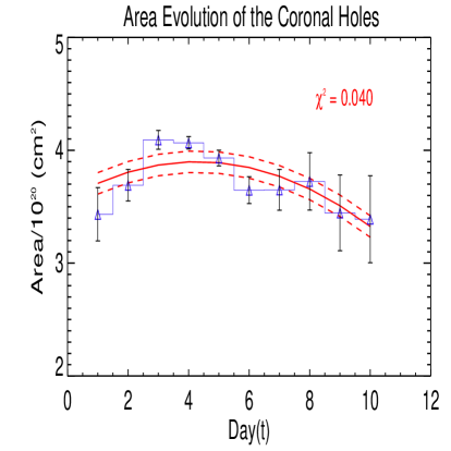
| A | 3.57 | 0.83 | 0.15 | 0.30 | -0.02 | 0.02 | 0.040 |
| F | 6.06 | 0.30 | 2.97 | 0.70 | -0.20 | 0.06 | 0.054 |
| F1 | 3.70 | 0.90 | 0.23 | 0.10 | -0.03 | 0.01 | 1.721 |
| T | 0.91 | 0.30 | 0.02 | 0.04 | -0.001 | 0.004 | 0.017 |
| Parameters | C0 | C0 | C1 | C1 | C2 | C2 | |
|---|---|---|---|---|---|---|---|
| A | 3.70 | 0.98 | 0.80 | 0.70 | -0.02 | 0.01 | 0.152 |
| F | 5.40 | 1.20 | 4.30 | 0.90 | -0.50 | 0.09 | 0.103 |
| F1 | 1.80 | 1.80 | 1.30 | 0.90 | -0.14 | 0.09 | 0.052 |
| T | 0.90 | 0.30 | 0.50 | 0.10 | -0.05 | 0.01 | 0.003 |
| Parameters | C0 | C0 | C1 | C1 | |
|---|---|---|---|---|---|
| A | 3.80 | 0.50 | -0.50 | 0.10 | 1.409 |
| F | 1.30 | 0.08 | 0.50 | 0.20 | 6.986 |
| F1 | 4.40 | 0.30 | 0.70 | 0.50 | 0.405 |
| CT | 0.93 | 0.40 | 0.17 | 0.14 | 0.041 |
| CP | 0.97 | 0.20 | 0.17 | 0.15 | 0.041 |
| Photospheric | 4.27 | 0.22 | 3.67 | 0.90 | 4.474 |
| Corona | 0.075 | 0.020 | 0.09 | 0.04 | 0.610 |
| MP | 0.18 | 0.04 | 0.77 | 0.15 | 2.478 |
| TP | 0.97 | 0.10 | 0.03 | 0.10 | 0.041 |
| True temperature | 0.94 | 0.10 | 0.03 | 0.01 | 0.041 |
| Parameters | C0 | C0 | C1 | C1 | |
|---|---|---|---|---|---|
| A | 3.80 | 0.50 | +0.50 | 0.10 | 1.409 |
| F | 3.00 | 0.20 | 2.60 | 0.20 | 3.744 |
| F1 | 5.20 | 0.10 | 5.10 | 1.00 | 1.559 |
| CT | 0.90 | 0.10 | 0.40 | 0.01 | 0.857 |
| CP | 0.93 | 0.10 | 0.50 | 0.10 | 0.857 |
| Photospheric | 4.21 | 0.22 | 1.32 | 0.90 | 4.162 |
| Corona | 0.08 | 0.01 | 0.03 | 0.01 | 4.162 |
| MP | 2.40 | 0.10 | 3.40 | 0.20 | 0.032 |
| TP | 0.01 | 0.001 | 0.0002 | 0.0001 | 2.481 |
| True temperature | 1.01 | 0.01 | 0.02 | 0.03 | 2.481 |
3 RESULTS
As in the previous study (Hiremath & Hegde 2013), we follow the similar criteria in selection of coronal holes and adopt similar method in binning the CH data for different latitudes. A typical coronal hole in the north-eastern quadrant of the SOHO/EIT image observed on 1st Jan 2001 is presented in Fig 1(a). Whereas separated coronal hole with its boundary detected from the threshold criterion (see the details in section 2 of Hiremath & Hegde 2013) is presented in Fig 1(b). We define apparent life span (as actual life span is larger) as number of observed days that have first and last appearance of CH on the same side of solar disk. In this way, for the observed coronal holes with different life spans (minimum of 4 days to maximum of 10 days) that appear at different latitudes and between +65∘ to -65∘ longitude from the central meridian are illustrated in Fig 2(a). With the constraint that coronal holes that occur between +40∘ (northern hemisphere) to -40∘ (southern hemisphere) latitude zones, 113 coronal holes with different life spans ultimately yield totally 796 data points for the present analysis. As the minimum life span of coronal hole is 4 days, transient coronal holes (that have life span 2 days; Kahler and Hudson 2001) that might have different physical properties are not included in this analysis. Irrespective of their life spans and after binning the coronal holes between 0-5∘, 5-10∘, etc., average latitudes of CH are computed. Fig 2(b) illustrates the idea of how totally 796 observed data points are distributed in different latitude bins.
For the typical two coronal holes (first CH is observed in the southern (latitude ) hemisphere and second CH is observed in the northern (latitude ) hemisphere respectively), following the methods presented in section 2, daily estimated different physical parameters are presented in Table 2. For the sake of comparison of temperature structure of CH computed from our method, by employing filter ratio technique, we also computed temperature structure. For example, Hinode/XRT data of 12/02/2007 and 15/08/2007 taken in Al-mesh/Al-poly filters are considered for temperature measurement. We followed the filter ratio method of Narukage et al. (2011) and temperature structure of these two CH is estimated. We find that temperature structure of CH estimated by our method and temperature structure of CH estimated by method of Narukage et al. (2011) is of the same order. With this confidence in mind that both the methods yield the same temperature structures, for all the 113 coronal holes considered for this study, we compute all the physical parameters (as defined in section 2) and are illustrated in Figs. 4-11.
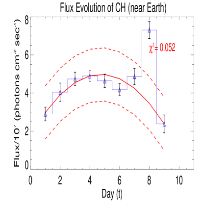
Our first objective is to understand daily evolution of coronal hole during its passage over the observed solar disk. For example, irrespective of their life spans and latitudes, for longitudes between +65∘ to -65∘, that are combined together in both the latitudes, Fig 4. illustrates the daily evolution of area (A), radiative flux (F) on the sun, radiative flux near the Earth (to be specific at Lagrangian point where SOHO space craft is positioned) () and temperature structure (T) of CH on the sun. Polynomial of degree 2 (quadratic) yields the best fit for the daily variation of CH. Different estimated parameters (, and ) of the polynomial fit with their respective uncertainties (, and ) and, (a measure of goodness of fit) values are presented in Table 3 (+65 to -65 deg longitudes) and in Table 4 (+45 to -45 deg longitudes) respectively.
It is to be noted that , daily variations of radiative flux of CH may be useful for the Earth’s ionospheric studies (Bauer 1973; Hinteregger 1976; Roble and Schmidtke 1979; Richards, Fennelly, Torr 1994; Lilensten et.al. 2007; Dudok de Wita and Watermanna 2010; Kretzschmar et.al. 2009). According to Bauer (1973), one of the principal ionizing radiation (others are solar x-ray photons, galactic cosmic rays, solar cosmic ray protons, etc.) responsible for formation of planetary ionospheres is solar EUV. Although all the EUV photons from sun’s whole disk can ionize the planetary atmospheres, EUV photons from coronal holes have more momentum that probably disturb the ambient planetary ionospheres. That means, probably transient behavior of EUV photons of the coronal holes leads to transient or sudden disturbances in the planetary ionospheres.
From observations of EUV images one can argue that much brighter surrounding coronal hole must be responsible for ionizing the Earth’s upper atmosphere rather than a dark coronal hole. However, there is a difference in these two images. Compared to surrounding brighter region of coronal holes, radiation emitted from the coronal hole is mainly associated with fast solar wind, accompanied by increase in temperature, is more effective in ionizing the Earth’s atmosphere and also leading to geomagnetic disturbances.
3.1 Estimation Life Span of CH
As for solar physics point of view, it is interesting to estimate the actual life span of coronal holes. If we consider daily variation of area of CH on the solar disk, best fit yields the quadratic equation with respect to time. As a first approximation, we can crudely estimate average life span of CH although individual coronal holes may have different life spans. After neglecting the non-linear term (as it is very small, see Figures 4 and 5 and, Table 3 and 4) and assuming that daily variation of area curve is symmetric (with respect to maximum area), for area of CH to be zero when it decays completely, average life span is estimated to be 46 days.
3.2 Estimation of Magnetic Diffusivity of Corona
From this daily evolution area curve, we find the average area from which average diameter (assuming that area is circular) of CH is estimated to be cm. Further making assumption that CH is a magnetic flux tube whose area evolution is only dictated by magnetic diffusion, magnetic diffusivity (=, where is life span) of the corona is estimated to be /sec which is very close to estimates of previous studies (Krista 2011; Krista et.al. 2011; Hiremath and Hegde 2013). Similarly neglecting the second non-linear coefficient (which is not significant as the error is of same order) in the empirical law of area that is derived from the least square fit (Fig. 4), one can estimate the area derivative and by employing the derived area derivative law (=) from the previous study (Hiremath and Hegde 2013; see the section 4), magnetic diffusivity of the corona is estimated to be of similar order ( /sec), as estimated above. Interestingly and it is to be noted that magnetic diffusivity estimated by our both the methods and magnetic diffusivity estimated by the previous studies (Krista 2011; Krista et.al. 2011) are of the same order.
3.3 Thermal and Magnetic Field Structures of the Coronal Holes
Knowing thermal structure is very important in understanding the fast solar wind emanating from the coronal hole (Hegde et al. 2015 and references there in). It is also important to examine whether thermal structure of coronal is independent or dependent on the latitude which in turn may give clue as to why high latitude coronal holes have high solar wind velocity compared to the low latitude or equatorial coronal holes (McComas, Elliott and Steiger 2002) during the minimum period. It is also interesting to know whether from thermal pressure of coronal hole (if CH is a magnetic flux tube, the CH pressure is combination of plasma and magnetic pressure) one can separate the magnitude of average magnetic field structure of coronal holes at the corona. These important observed physical parameters such as thermal and magnetic structures are essential to probe the depth (Hiremath and Hegde 2013) and structure of the coronal holes. In the following study, first by estimating the radiative flux, with the assumption of thermodynamic equilibrium, we estimate the temperature structure. This temperature structure we call as total temperature. This assumption of thermodynamic equilibrium is almost akin to the same assumption employed in differential emission measure (for example Hahn, Landi and Savin 2011 ) in estimating temperature structure of coronal holes. Further by using the observed density of CH, we compute the total pressure. The obvious reason for calling total pressure is that CH is a magnetic flux tube whose total pressure is the combination of thermal and magnetic pressures. This concept basically is invoked from the Parker’s (1955) idea wherein if magnetic flux tube is in hydrostatic equilibrium, a combination of gas and magnetic pressure in the flux tube is balanced by the external gas thermal pressure. In the following section, by using information of estimated total temperature and pressure, we not only derive the actual temperature structure but also estimate the average magnetic field structure of the coronal hole.
3.3.1 Latitudinal Variation of Thermal Structure of Coronal Hole
Many previous studies (Zhang et al. 2007; Landi 2008 etc.) concentrated on single coronal hole and estimated average temperature structure. As for our knowledge, this is a first study which uses many coronal holes for estimating the thermal structure. Following the previous study (Hiremath and Hegde 2013) in selecting the data, first we estimate the different physical parameters of CH that occur between +65∘ to -65∘ longitudes from the central meridian. Following the method described in section 2 and irrespective of their areas and number of observed days on the solar disk, for different latitudes, variation of different physical parameters such as area, radiative flux (on the sun and near Earth) and total temperature structure are presented in Fig 6. For example, one can notice from the least-square fit (of the form , where is latitude, and constants and, Y represents different physical parameters) of area-latitude curve that, on average, equatorial coronal holes have large area compared to high latitude coronal holes. Whereas other illustrations of radiative flux and temperature structures follow inverse latitudinal variations, rather than following similar area-latitude relationship. Inconsistency of both these results probably could be due to contribution of coronal holes that are near +65∘ to -65∘ longitudes, close to the limb. Hence, in order to completely minimize such projectional effects, further we restricted the data of CH that occur between +45∘ to -45∘ longitudes from the central meridian and the same results that are presented in Fig 6 are also presented in Fig 9. It is to be noted that although there is more variation, especially in case of Figures 9(c) and 9(d), over all trend of least square fits for all the Figures is same (of the form ). Whereas, in case of illustrations 6, except Figures 6(b)-6(d), law of least square fit for Figure 6(a) is different (of the form ). However, one can notice from Fig 9 that inconsistency in latitudinal variation of area and flux curves is removed and all the illustrations have same latitudinal variations.
Latitudinal variation of different physical parameters of CH are subjected to least square fit (of the the form ) and estimated coefficients and with their respective uncertainties and values are presented in Tables 5 and 6 respectively. In both the tables, with the units in cgs, first column consists of area (A), radiative flux (F) on the sun, flux (F1) near earth, total temperature (CT), total pressure (CP), strength of coronal hole magnetic field structure at the photosphere () and at the corona () and, magnetic pressure (MP) of the coronal hole at corona, actual pressure (TP) and temperature of the coronal hole at the corona. Whereas second to fifth columns represent the coefficients and their uncertainties as estimated by the least square fit. The last column in both the tables represents the value of (a measure of goodness of fit).
Although variation of thermal structure (for example observed inferences: David et.al. 1998; Landi 2008; Landi and Cranmer 2009; Hahn, Landi and Savin 2011 and, theoretical inferences: Osherovish et.al. 1985) of the coronal hole at different heights in the corona is available, studies on latitudinal variation of thermal structure of coronal holes are not available. In this respect, we believe that, our results on latitudinal variation of thermal structure of coronal holes will be very useful to the solar community.
3.3.2 Estimation of Strength of Magnetic Field Structure of the Coronal Holes
From the latitudinal variation of total temperature and the observed density structure (Doschek et al. 1997 etc.) of coronal holes, with respect to latitude, total pressure (, where is number of electron density, is Boltzmann constant and is estimated total temperature; it is assumed that coronal hole plasma has same number of electrons and protons density hence the number is multiplied) is estimated and is presented in Fig 7(a) (for the +65∘ to -65∘ longitudes). In order to minimize the projectional effects, same parameter (for the +45∘ to -45∘ longitudes from the central meridian) is presented in Fig 10(a). One can notice from both the figures that latitudinal variation of total pressure of the coronal hole depends upon the latitude such that equatorial coronal holes have low pressure compared to high latitude coronal holes. In case one accepts that coronal hole is a magnetic flux tube, then total pressure in the coronal hole is sum of plasma and magnetic pressures. Offcourse, best analogy (except strong magnetic fields in sunspots) between magnetic flux tubes (sunspots) and coronal hole can be obtained from the previous (Fla et.al. 1984; Davila 1985; Cally 1986, 1987; Osherovich et.al., 1985; Ofman 2005 and references there in; Obridko and Solovev, 2011) MHD models.
Hence, if we accept that plasma pressure of coronal hole is independent of latitudes, then one possible interpretation for latitudinal variation of total pressure of the coronal holes could be due to contribution from the magnetic pressure. That means if one knows the latitudinal variation of magnetic field structure of coronal holes, one can compute the magnetic pressure and can be subtracted from the estimated total pressure. Unfortunately, to the knowledge of the authors, there are no such studies that give the information of latitudinal variation of magnetic field structure of coronal holes at the corona. For this purpose, we adopt the following method in computing the magnetic field structure and hence magnetic pressure of the coronal hole at the corona.
First we make the reasonable assumption that coronal hole is a magnetic flux tube that probably anchored below the photosphere (Gilman 1977; Golub et.al 1981; Jones 2005; Hiremath and Hegde 2013). As the magnetic flux tube is embedded in the solar atmosphere, increase with height from photosphere to corona results in decrease of surrounding ambient plasma pressure and hence tube must expand. In the following, this statement can further be corroborated from the previous study (Hegde, Hiremath and Doddamani 2014). With the SDO data, for the coronal hole observed in three wavelengths 174 , 193 and 211 , average area of coronal hole are : for 174 , for 193 and, for 211 respectively. Simultaneously DN counts (radiative intensity) also reduce from 174 , 193 and 211 respectively. Successive increase of line formation (Yang et.al. 2009) for 174 , 193 and 211 at different heights are: 1.01, 1.05 and 1.3. One can notice that within the 30% of solar radius from the photosphere, coronal hole’s area increases twice the area of coronal hole at the photosphere. Considering these facts it is reasonable to consider the coronal hole is expanding from photosphere to corona where 195 line originates.
Further if one accepts that coronal hole is a Parker’s flux tube (Parker 1955), then magnitude of magnetic field structure inside the coronal hole is directly proportional to (where is external ambient pressure of the plasma). Hence, with this simple relationship, one can estimate strength of magnetic field structure of the coronal hole at the corona if one knows the strength of magnetic field structure and ambient plasma pressures at different heights. To be specific, the resulting derivation will be (that is obtained from the above simple relationship) Bc=Bpho ()1/2 (where and are strength of magnetic field structure of the coronal hole and ambient plasma pressure at the corona and, Ppho and Bpho are strength of magnetic field structure of the coronal hole and ambient plasma pressure at the photosphere). As for strength of magnetic field structure of coronal hole at the photosphere, for the same time of observation and latitude, we consider the inferred values at the photosphere (using Solar Monitor website). This inferred field from the photospheric magnetograms is the line of sight component. Then with the above formula and, by using the ambient external pressure at the photosphere and the corona (Aschwanden 2004), magnetic field structure (and hence magnetic pressure ) of the coronal hole at the corona (around 1.1 , where the 195 line is originated) is estimated.
After binning in different latitude zones, latitudinal variation of average strength of magnetic field structure of coronal hole at the photosphere are presented in Fig 7b (for +65∘ to -65∘ longitudes) and in Fig 10b (for +45∘ to -45∘ longitudes). It is interesting to note that, as we reasoned above, indeed magnitude of magnetic field structure (and magnetic pressure) of the coronal hole at the photosphere increases from equator to higher latitudes although curve of Fig 10(b) appears to be flatter. Estimated strength of magnetic field structure of the coronal hole and its magnetic pressure at the corona are presented in Figures 7(c) and 7(d) (for +65∘ to -65∘ longitudes) and in Figures 10(c) and 10 (d) (for +45∘ to -45∘ longitudes). One can notice that, on average, magnitude of magnetic field structure of coronal hole at the corona is estimated to be 0.08(0.02) Gauss.
Offcourse, one can argue from the spatially resolved individual coronal holes that this estimated field strength depends on whether the coronal holes are in new active regions where the fields are strong or in old expanded unipolar regions where the fields are weak. However, our estimated strength of magnetic field structure is derived from the least square fit (first coefficient of the linear fit) with many coronal holes rather than obtaining the spatial information.
There are also other possibilities that this estimated strength of magnetic field is possibly different than the actual strength of magnetic field structure for the following two reasons. Firstly observed magnetic field structure of the coronal hole estimated from the photospheric magnetogram is longitudinal and hence inferred magnetic field of the coronal hole at corona is also a longitudinal component. Whereas for the radial component of magnetic field (such a field structure is invoked in modeling of coronal hole), strength of longitudinal component of magnetic field of coronal hole appears to be under estimated as radial field is (where is longitudinal component of magnetic field, is latitude (that varies 0 to 90 deg from equator to pole) and is inclination angle of rotational axis of the sun). Secondly and according to Parker’s (1955) Flux tube model, estimated strength of magnetic field depends upon square root of ambient pressure which ultimately is model dependent. Hence, it can not be ruled out that some amount of uncertainty (0.01, ) persists that is reflected in the estimated strength of longitudinal component of magnetic field from the least square fit. However, it is important to be noted that we haven’t come across any study that estimates strength of magnetic field of the coronal hole observed in 195 .
By knowing latitudinal variation of strength of magnetic field structure of the coronal hole, the estimated magnetic pressure is subtracted from the total pressure of the coronal hole and actual thermal pressure of the coronal hole is computed. By knowing electron density and thermal pressure (Figures 8(a) and 11(a)), actual temperature structure of corona hole is computed and latitudinal variation of the same is presented in Fig 8(b) (for +65∘ to -65∘ longitudes) and in Fig 11(b) (for +45∘ to -45∘ longitudes) respectively. From these figures, we find that variation of temperature structure of coronal holes is independent of solar latitudes.
6(a) 6(b)


 |
 |
6(c) 6(d)
7(a) 7(b)


 |
 |
7(c) 7(d)
8(a) 8(b)


9(a) 9(b)


 |
 |
9(c) 9(d)
10(a) 10(b)


 |
 |
10(c) 10(d)
11(a) 11(b)


4 Discussion and conclusions
There are two very interesting results that need worthy to be discussed here. First result is the magnitude of magnetic field structure of coronal holes that increases from equator to both poles of the sun. One can argue from the previous studies (Harvey et al 1982; Webb and Davis 1985; Abramenko et.al 2009) that this result could be due to occurrence of coronal holes during the evolution of solar cycle as the polar coronal holes have stronger magnetic fields than the coronal holes at low latitudes. Although inferred result of latitudinal variation of strength of magnetic field structure of coronal holes from the present study is consistent with the results of previous studies, question remains why high latitude coronal holes occur with high average magnetic field strengths than the low latitude coronal holes.
This important observed and inferred information of latitudinal variation of strength of magnetic field probably suggests coronal holes’ origin that is not consistently understood. As the coronal holes are unipolar magnetic field structures, their origin can be understood from the global nature of magnetic field structure of the sun. Probably, we believe, following conjecture on genesis of coronal holes is consistent with the result of latitudinal dependency of magnitude of magnetic field structure of the coronal holes.
During the period of minimum solar activity, white light pictures taken during total solar eclipse, one can notice the dipole like magnetic field structure delineated along the intensity patterns (rays) that are originated from the two poles. Infact observational (Stenflo 1993) and theoretical studies (Hiremath and Gokhale 1995 and, references there in) can not rule out such a large-scale global dipole like magnetic field structure, may be of primordial origin. Offcourse we have to make a clear distinction between the “steady” and “time dependent” parts of solar magnetic field structure. “Steady” part of solar magnetic field structure has a time scale of billion of years (Hiremath and Gokhale 1995 and reference therein). Whereas time dependent part of solar magnetic field structure has a 22 yrs time scale. For understanding genesis of coronal hole, in the following conjecture, we invoke the large-scale “steady” part of the magnetic field structure in order to be compatible with the inferred latitudinal variation of magnetic field structure of the coronal hole.
Observational (Stenflo 1993) estimates yield the intensity to be 1 G. Whereas, for matching of 22 year of magnetic periodicity, previous study (Hiremath and Gokhale 1995 and, references there in) estimates sun’s global dipole like magnetic field structure to be 0.01 G. This result is also consistent with the recently estimated average magnetic field structure of the 0.028 G (Kotov 2015). Although genesis of coronal holes is debatable, for the consistency of inferred coronal hole magnetic field structure whose intensity increases from equator to pole, we present probable mechanism of CH formation as follows.
If the large-scale coronal poloidal magnetic field structure is perturbed, Alfven waves are produced whose interference pattern leads to formation of coronal hole structure. If is intensity of large-scale steady part of magnetic field structure, then resulting amplitude of Alfven waves is same order as that of intensity of original magnetic field structure. That is is . Although steady part of poloidal part of magnetic field structure probably consists of combined (uniform, dipole and quadrupole) filed structure (Hiremath and Gokhale 1995), for the sake of simplicity, let us consider dipole like field structure only. For a particular radius, intensity or magnitude of magnetic field structure varies as (where is observed latitude; here =0∘ is equator and =90∘ is pole) whose magnitude increases from equator to pole. That means, as presented in Figures (7(c) and 10(c)), coronal holes originated at the equator must have less magnitude of magnetic field structure compared to the coronal holes that originate near the poles. If one accepts a naive concept that coronal holes are formed due to Alfven wave perturbations of poloidal component of magnetic field structure, as the amplitude of magnetic field structure of Alfven waves is at least same order as that of steady part of magnetic field structure, hence it is not surprising that average (see the fits) strength of magnetic field structure is same as strength (in the range of 0.01-1 G) of steady magnetic field structure as estimated by observational (Stenflo 1993; Kotov 2015) and theoretical (Hiremath and Gokhale 1995) studies. It is to be noted that this speculative explanation for the origin of coronal holes has to be treated cautiously unless some other studies also agree with our conjecture that coronal holes originate from the Alfven perturbations of global large-scale magnetic field structure.
Another interesting result is that variation of thermal structure (especially actual temperature) of coronal holes is independent of latitudes. As coronal hole is a magnetic flux tube, for the steady state of magnetic field structure and no gain of magnetic flux during coronal hole evolution, condition of infinite conductivity leads to isorotation of coronal holes with the surrounding ambient plasma rotation. That means coronal hole magnetic flux bundle follows the path of isorotational contours. To be precise, coronal holes that might have formed due to Alfven wave perturbations travel along the large scale magnetic field structure parallel to isorotational contours. Infact, in the previous study (Hiremath and Gokhale 1995), we have shown that large-scale magnetic field structure, may be of primordial origin, consists of combined magnetic field structure in the radiative core and current free (combination of dipole and quadrupole like field structures that are embedded in the uniform) field structure in the convective envelope and both the structures in turn isorotate with the internal solar plasma rotation as inferred by the helioseismology.
From the above discussion, it is clear that rotation rate of coronal holes and rotation rate of ambient solar plasma depend upon each other. Helioseismic inferences (Hiremath 2013, 2016 and references there in) yield rigid body rotation in the radiative core and differential rotation in the convective envelope. That means if coronal holes originate only in the convective envelope, they must rotate differentially. Otherwise coronal holes likely to rotate rigidly if coronal holes originate in the radiative core. On the theoretical (Gilman 1977; Golub et. al. 1981; Jones 2005) and observational (Hiremath and Hegde 2013) inferences, it is argued that coronal holes probably originate below the convective envelope which in turn implies that coronal holes rotate rigidly (as the radiative core rotates rigidly). On other hand, by evolving magnetic diffusion equation, Wang and Sheeley (1993) simulate the rotation rate of the coronal holes from the current free nature of the coronal field that is rotating with the distorted active region fields.
If one considers curl of momentum equation in the cylindrical coordinates and for steady angular velocity gradient, angular velocity of solar plasma is balanced (Chandrasekhar 1956; Brun, Antia and Chitre 2010 and references there in) by the combined forces due to stretching/tilting of vorticity due to velocity gradients, advection of vorticity by the flows, turbulent and Reynold stresses, Maxwell stresses, baroclinic forces, etc. If one assumes other forces are negligible, then gradient of angular velocity is balanced by the baroclinic forces only. In cylindrical coordinates, the relationship can be expressed in the form of equation , where is angular velocity of the solar plasma, is acceleration due to gravity, is specific heat at the constant pressure, is the adiabatic temperature gradient, is the radial variation and is entropy of the ambient medium. This equation is called thermal wind balance equation (Brun, Antia and Chitre 2010). That means, unless there is a temperature difference between the pole and equator, angular velocity of the solar plasma can not be differential with respect to latitude and also can not be maintained. As the coronal holes isorotate with the solar plasma, this equation also implies that unless there is a temperature structure that varies from equator to pole, coronal holes can not rotate rigidly. However, present study yields the temperature structure (and hence entropy) of coronal holes independent of solar latitude. Hence, above thermal wind balance equation implies that =0. That means coronal holes must rotate rigidly or rotation rate of coronal holes is independent of solar latitude. Infact this reasoning also matches with the recent results (Hiremath and Hegde 2013) of rigid body rotation rates of coronal holes derived from the SOHO 195 data.
To conclude this study, for the years 2001-2008, near equatorial coronal holes detected from the SOHO/EIT images are used to understand the area evolution and, latitudinal variation of thermal and magnetic field structure. Different estimated physical parameters of the coronal holes are: area , radiative flux at the sun photons , radiative energy ergs , temperature structure K and magnitude of magnetic field structure estimated to be G.
Acknowledgments
This work has been carried out under “CAWSES India Phase-II program of Theme 1” sponsored by Indian Space Research Organization(ISRO), Government of India. SOHO is a mission of international cooperation between ESA and NASA.
REFERENCES
Abramenko, V., Yurchyshyn, V & Watanabe, H. 2009, Sol. Phys., 260, 43
Aschwanden, M, J., 2004, Physics of the Solar Corona - An Introduction, Praxis Publishing Ltd., Chichester, UK, and Springer-Verlag Berlin
Bauer, S. J., 1973, in Physics of Planetary Ionospheres, Springer-Verlag, p. 47
Bohlin, J. D. 1977, Sol. Phys., 51, 377
Brun, A. S., Antia, H. M. & Chitre, S. M., 2010, A&A, 510, 33
Cally, P. S. 1986, Sol. Phys., 103, 277
Cally, P. S. 1987, Sol. Phys., 108, 183-
Chandrasekhar S.,1956, ApJ, 124, 231
Chiuderi, D. F., Avignon, Y & Thomas, R. J., 1977, Sol. Phys., 51, 143
Chiuderi, D. F., Landi, E., Fludra, A. & Kerdraon, A., 1999, A&A, 348, 261
Choi, Y., Moon, Y.-J., Choi, S., Baek, J.-H., Kim, S. S., Cho, K.-S., & Choe, G. S. 2009, Sol. Phys., 254, 311
Cranmer, S.R. 2009, Living Reviews in Sol. Phys., 6, 3
David, C., Gabriel, A. H., Bely-Dubau, F., Fludra, A., Lemaire, P. & Wilhelm, K. 1998, A&A, 336, L90
Davila, J. M. 1985, ApJ, 291, 328
Delaboudiniere, J. P. et al. 1995, Sol. Phys., 162, 291
Doschek, G. A. & Feldman, U. 1977, ApJ, 212, L143
Doschek, G. A., Warren, H. P., Laming, J. M., Mariska, J. T., Wilhelm, K., Lemaire, P., Schuehle, U., & Moran, T. G. 1997, ApJletters, 482, 109
Doschek, G. A. & Laming, J. M. 2000, ApJ, 539, L71
Doyle, J. G., Chapman, S., Bryans, P., Pérez-Suárez, D., Singh, A., Summers, H. & Savin, D. W. Research in Astronomy and Astrophysics, 10, 91, 2010
Dudok de Wita, T & Watermanna, J., 2010, Comptes Rendus Geoscience 342, 259
Dwivedi, B. N & Mohan, A., 1995, Sol. Phys., 156, 197
Dwivedi, B. N., Mohan, A & Wilhelm, K. 2000, Advances in Space Research, 25, 1751
Esser, R., Fineschi, S., Dobrzycka, D., Habbal, S. R., Edgar, R. J., Raymond, J. C., Kohl, J. L. & Guhathakurta, M. 1999, ApJ, 510, L63
Fathy, I., Amory-Mazaudier, C., Fathy, A., Mahrous, A. M., Yumoto, K. & Ghamry, E. 2014, Journal of Geophysical Research: Space Physics, 119, 4120
Fla, T., Habbal, S. R., Holzer, T. E & Leer, E. 1984, ApJ, 280, 382
Gilman, P. A. 1977, Coronal holes and high speed wind streams Conference, ed. Zirker, J. B. 331
Golub, L., Rosner, R., Vaiana, G. S., & Weiss, N. O. 1981, ApJ, 243, 309
Guennou, C.; Auchère, F.; Soubrié, E.; Bocchialini, K.; Parenti, S & Barbey, N. 2012, ApJS, 203, 26, 14
Habbal, S. R., Esser, R., & Arndt, M. B. 1993, Sol. Phys., 413, 435
Habbal, S. R. 1996, Solar and Interplanetary Transients, proceedings of IAU Colloquium 154, edited by S. Ananthakrishnan; A. Pramesh Rao., p. 49
Hahn, M., Landi, E., & Savin, D. W. 2011, ApJ, 736, 101
Hara, H., Tsuneta, S., Acton, L. W., Bruner, M. E., Lemen, J. R. & Ogawara, Y. 1994, PASJ, 46, 493
Hara, H., Tsuneta, S., Acton, L. W., Bruner, M. E., Lemen, J. R. & Ogawara, Y. 1996, Advanced Space Research, 17, 4
Harvey, J. W. & Sheeley, N. R., Jr. 1979, Space Sci. Rev., 23, 139
Harvey, K. L., Harvey, J. W., & Sheeley, N. R., Jr. 1982, Sol. Phys., 79, 149
Hegde, M., Hiremath, K. M., Doddamani, V. H., Gurumath, S. R. 2015, Journal of Astrophysics and Astronomy, 36, 355
Hegde, M., Hiremath, K. M., Doddamani, V. H. 2014, Advances in Space Research, 54, 272
Hiremath, K. M. 1994, Study of Sun’s Long Period Oscillations, Ph.D Thesis, Bangalore University, 1994, p. 142, http://prints.iiap.res.in/handle/2248/122
Hiremath, K. M & Gokhale, M. H. 1995, ApJ, 448, p.437
Hiremath, K. M. 2001, Bulletin of the Astronomical Society of India, 29, 169
Hiremath, K. M & Mandi, P. I. 2004, New Astronomy, 9, 651
Hiremath, K. M. 2009, Sun and Geosphere, 4, 16
Hiremath, K. M. 2013, in Seismology of the Sun: Inference of Thermal, Dynamic and Magnetic Field Structures of the Interior, 2013, p. 333, springer
Hiremath, K. M., & Hegde, M. 2013, ApJ, 763, 137
Hiremath, K. M., Hegde, M., & Soon, W. 2015, New Astronomy, 35, 8
Hiremath, K. M. 2016, in Cartography of the Sun and the Stars., Eds: Rozelot, Jean-Pierre, Neiner, Coralie, p. 85
Hegde, M., Hiremath, K. M., Doddamani, V. H. & Gurumath, S. R. 2015, Journal of Astrophys and Astronomy, 36, 355
Hinteregger, H. E. 1976, Journal of Atmospheric and Terrestrial Physics, 38, 791
Insley, J.E., Moore, V., & Harrison, R.A. 1995, Sol. Phys., 160, 1
Japaridze, D. R., Bagashvili, S. R., Shergelasvili, B. M., Chargeishvili, B. B. 2015, Astrophysics, 58, 575
Jones, H. P. 2005, Large-scale Structures and their Role in Solar Activity ASP Conference, eds, Sankarasubramanian, K., Penn, M., & Pevtsov, A. 346, 229
Kahler, S. W & Hudson, H. S. 2001, J. Geophys. Res., 106, A12, 29239
Karachik, N. V & Pevtsov, A, A. 2011, ApJ, 735, 6
Kotov, V. A., 2015, Advances in Space Research, 55,979
Kretzschmar, M., Dudok de Wita, T., Lilensten, J., Hochedez, J.-F., Aboudarham, J., Amblard, P.-O., Auchère, F, & Moussaoui, S. 2009, Acta Geophysica, 57, 42
Krieger, A.S., Timothy, A.F., & Roelof, E.C. 1973, Sol. Phys., 29, 505
Krista, L. D. 2011, Ph.D. Thesis, University of Dublin, Trinity College
Krista, L. D., Gallagher, P. T., & Bloomfield, D. S. 2011, ApJ, 731, 26
Landi, E. 2008, ApJ, 685, 1270
Landi, E., & Cranmer, S. R. 2009, ApJ, 691, 794
Landi, E., Reale, F., & Testa, P. 2012, A&A, 538, 10
Lei, J., Thayer, J. P., Forbes, J. M., Sutton, E. K., & Nerem, R. S. 2008, Geophys. Res. Lett., 35, L19105
Lilensten, J., Dudok de Wita, T., Amblard, P.-O., Aboudarham, J., Auchère, F., Kretzschmar, M., Annales Geophysicae, 2007, 25, 1299
Machiya, H. & Akasofu, S.-I. 2014, Journal of Atmospheric and Solar-Terrestrial Physics, Volume 113, 44
Marsch, E., Tu, C.-Y., & Wilhelm, K. 2000, A&A, 359, 381
McComas, D. J., Elliot, H. A & von Steiger, R. 2002, Geophys.Res.Lette., 29, 28
Mogilevsky, E. I., Obridko, V. N., & Shilova, N. S. 1997, 176, 107
Moses, D., Clette, F., Delaboudini‘ere, J-P. et al. 1997, Sol. Phys., 175, 571
Narukage, N., Sakao, T., Kano, R., Hara, H., Shimojo, M., Bando, T., Urayama, F., Deluca, E., Golub, L., Weber, M., Grigis, P.,
Navarro-Peralta, P. & Sanchez-Ibarra, A. 1994, Sol. Phys., 153 Cirtain, J. & Tsuneta, S. 2011, Sol. Phys., 269, 169
Neupert, W.M. & Pizzo, V. 1974, J. Geophys. Res., 79, 3701
Nistico, G., Patsourakos, S., Bothmer, V., Zimbardo, G., Advances in Space Research, 48, 1490-
Nolte, J. T., Krieger, A. S., Timothy, A. F., Gold, R. E., Roelof, E. C., Vaiana, G., Lazarus, A. J., Sullivan, J. D., & McIntosh, P. S. 1976, Sol. Phys.46, 303
Obridko, V. N. & Shelting, B. D. 1989, Sol. Phys., 124, 73
Obridko, V. N & Solov’ev, A. A. 2011, Astronomy Reports, 55, 1144
Ofman, L. 2005, Space Science Reviews, 120, 67
Osherovich, V. A.; Gliner, E. B.; Tzur, I.; Kuhn, M. L. 1985, solar physics, 97, 251
Parker, E. N. 1955, ApJ, 121, 491
Peter, H. & Judge, P. G. 1999, ApJ, 522, 1148
Ram, S. T., Liu, C. H., & S.-Y. Su. 2010, J. Geophys. Res., 115, 14
Roble, R. G. & Schmidtke, G. 1979, Journal of Atmospheric and Terrestrial Physics, 41, 53
Richards, P. G., Fennelly, J. A., & Torr, D. G. 1994, J. Geophys. Res., 99, 8981
Rotter, T., Veronig, A. M., Temmer, M. & Vršnak, B. 2012, Sol. Phys., 281,793
Shelke, R. N. & Pande, M. C. 1985, Sol. Phys., 95, 193
Shugai, Yu. S., Veselovsky, I. S., & Trichtchenko, L. D. 2009, Ge&Ae, 49, 415
Slemzin, V. A., Goryaev, F. F. & Kuzin, S. V. 2014, Plasma Physics Reports, Volume 40, 855
Sojka, J. J., McPherron, R. L., van Eyken, A. P., Nicolls, M. J., Heinselman, C. J., & Kelly, J. D. 2009, Geophys. Res. Lett., 36, L19105
Soon, W., Baliunas, S., Posmentier, E. S., & Okeke, P. 2000, NewAstronomy, 4, 563
Shugai, Y. S., Veselovsky, I. S & Trichtchenko, L. D. 2009, Geomagnetism and Aeronomy, 49, Issue 4, pp.415-424
Stenflo, J. O. 1993, in Solar Surface Magnetism, ed. R. J. Rutten & C. J. Shrijver (Dordrecht:Kluwer),8
Stucki, K., Solanki, S. K., Schühle, U., Rüedi, I., Wilhelm, K., Stenflo, J. O., Brković, A. & Huber, M. C. E. 2000, A&A, 363, 1145
Stucki, K., Solanki, S. K., Pike, C. D., Schühle, U., Rüedi, I., Pauluhn, A., & Brković, A. 2002, A&A, 381, 653
Timothy, A. F. & Krieger, A. S. 1975, Sol. Phys., 42, 135
Tu, C.-Y., Marsch, E., Wilhelm, K. & Curdt, W. 1998, ApJ503, 475
Verbanac, G., Vršnak, B., Veronig, A., & Temmer, M. 2011, A&A, 526, 20
Vršnak, B., Temmer, Ma Veronig, Astrid M. 2007, Sol. Phys., 240, 315
Wagner, W. J. 1975, ApJ, 198L, 141
Wagner, W. J. 1976, Basic Mechanisms of Solar Activity, Proceedings from IAU Symposium no. 71, edts. Bumba, V and Kleczek, J, p. 41
Wang, Y. M., Space Sci. Rev., 2009, 144, 383
Warren, H. P., Mariska, J. T., Wilhelm, K., ApJ, 1997, 490, L187
Webb, D. F. & Davis, J. M. 1985, Sol. Phys., 102, 177
Wiegelmann, T., Thalmann, J, K. & Solanki, S, K. 2014, The Astronomy and Astrophysics Review, 22, 106
Wilhelm, K., Marsch, E., Dwivedi, B. N., Hassler, D. M., Lemaire, P., Gabriel, A. H., & Huber, M. C. E. 1998, ApJ, 500, 1023
Wilhelm, K. 2006, A&A, 455, 697
Wilhelm, K. 2012, Space Sci. Rev., 172, 57
Xia, L. D., Marsch, E. & Wilhelm, K. 2004, A&A, 424, 1025
Yang, S.H., Zhang, J., Jin, C. L., Li, L. P and H. Y. Duan, H. Y. 2009, A&A, 501, 745
Zhang, J., White, S. M. & Kundu, M. R. 1999, ApJ, 527, 977
Zhang, H., Zhou, G., Wang, J. & Wang, H. 2007, ApJ, 655, L113
Zhang, J., Zhou, G., Wang, J., & Wang, H. 2007, ApJ, 655, L113
Zirker, J. B. 1977, Reviews of Geophysics and Space Physics, 15, 257